


1. Introduction
There is a general consensus that multiple cropping systems have superior yield potential over monocultures in agriculture and forestry (Gliessman, Reference Gliessman2015; Huang et al., Reference Huang, Liu, Heerink, Stomph, Li, Liu, Zhang, Wang, Li, Zhang, Van Der and Zhang2015; C.L.C. Liu et al., Reference Liu, Kuchma and Krutovsky2018; Maitra et al., Reference Maitra, Hossain, Brestic, Skalicky, Ondrisik, Gitari, Brahmachari, Shankar, Bhadra, Palai, Jena, Bhattacharya, Duvvada, Lalichetti and Sairam2021). However, experimental evidence of crop productivity enhancement in multi-crop (MC) systems has predominantly been confined to intercrops of no more than two species, compared to monocultures (e.g., Hamzei & Seyedi, Reference Hamzei and Seyedi2015; Morales-Rosales & Franco-Mora, Reference Morales-Rosales and Franco-Mora2009; Raza et al., Reference Raza, Khalid, Zhang, Feng, Khan, Hassan, Ahmed, Ansar, Chen, Fan, Yang and Yang2019; Runkulatile et al., Reference Runkulatile, Homma, Horie, Kurusu and Inamura1998; and the references in Maitra et al., Reference Maitra, Hossain, Brestic, Skalicky, Ondrisik, Gitari, Brahmachari, Shankar, Bhadra, Palai, Jena, Bhattacharya, Duvvada, Lalichetti and Sairam2021; Table 1). Evidence from combinations of three crops is scarce (Andersen et al., Reference Andersen, Hauggaard-Nielsen, Weiner and Jensen2007; Dapaah et al., Reference Dapaah, Asafu-Agyei, Ennin and Yamoah2003). The first experimental evidence of yield comparisons between MC farm plots with seven crop species and sole-crop (SC) plots of the same crop species, appeared in Deb (Reference Deb2021), revealed different degrees of efficiency of yield in different planting designs.
Deb’s (Reference Deb2021) study measured the yield advantage of MC plots over SC plots by the land equivalent ratio (LER) based on edible biomass yield per plant, although it is usually estimated by measuring yield per unit of land area under crop cover (Khanal et al., Reference Khanal, Stott, Armstrong, Nuttall, Henry, Christy, Mitchell, Riffkin, Wallace, McCaskill, Thayalakumaran and O’Leary2021; Mead & Willey, Reference Mead and Willey1980; Weigelt & Jolliffe, Reference Weigelt and Jolliffe2003). Here, we use both per plant (Yir [p]) andper unit area (Yir [a]) yields of the data from Deb (Reference Deb2021) to examine the sensitivity of LER with scaled units of measurement. In addition, we attempt to examine two more indices of yield advantages of MC farms planted to seven crops.
2. Methods and materials
2.1 Study sites
A total of eight farms in the State of Odisha, India, were selected for our experiments, whose details are given in Deb (Reference Deb2021). All these eight farms are owned by indigenous farmers, who traditionally grow 6–12 crop species on their farms every season. We chose seven crop species (S = 7) most commonly cultivated in the region, with zero synthetic agrochemical input. In addition to the seven species chosen for this experiment, a legume cover crop was planted on the farm margins. The yield of legumes was not included in this study, focusing instead on the seven different crops in each farm, compared to an SC plot of each of these seven species, separately grown. In this study, each replication of the eight farms includes three MC plots and seven SC plots.
2.2 Crop planting designs
As replacement designs are not practiced in real farms, and because replacement designs alter the individual crop densities, we chose to plant each crop species in equal proportions in all MC plots.
2.2.1 SC plot design
Two species of fruit crops (okra Abelmoschus esculentum and brinjal Solanum nigricum), three cereal crops (rice Oryza sativa ssp. indica, little millet Panicum sumatrense, and finger millet Eleusine coracana), and two leaf crops (red amaranth Amaranthus cruentus and green amaranth Amaranthus viridis) were planted in separate SC plots. The same cropping design was replicated in all the eight farms.
The SC plots were of the same size, and the crop plants were planted at a uniform spacing, with a planting density of 6.25 m−2 for brinjal saplings (40 cm × 40 cm), and 16 m−2 for all other crops (25 cm× 25 cm).
2.2.2 MC plot designs
A total of seven crop species were chosen for the MC farms. The crop species chosen for growing in the MC plots are: brinjal (BR), okra (OK), green amaranth (A1), red amaranth (A2), finger millet (FM), little millet (LM), and rice (RC).
In each farm, three designs (designated A, B, and C) of MC plots, composed of 21 × 21 cells, were established (Figure 1). Crop plants in Design A were arranged in a row intercropping system, planted to all the seven species arranged in successive rows, repeated three times over. Design B is nonrandom mixed cropping, where seven crop species were planted in a fixed order, with each cell diagonally matching the species in the previous row and column. Thus, each row and each column differed in crop combination, although the order remained the same, repeated three times over. Design C was also nonrandom mixed cropping, albeit with a different arrangement of crop species. Like that of Design B, diagonal cells repeated each crop, matching the previous row and column, repeating the arrangement three times over in both dimensions.
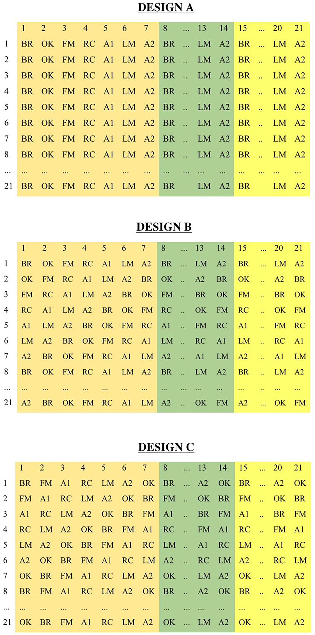
Figure 1. The planting designs A, B, and C for seven crop species. The numbers in the first column denote respective row numbers, and the numbers in the top row denote respective column numbers.
Legends: A1: green amaranth; A2: red amaranth; BR: brinjal; FM: finger millet; LM: little millet; OK: okra; RC: rice.
2.3 Crop area estimation
In all the plots, the spacing on each side of a crop is 40 cm for BR, and 25 cm for all other crops. Any crop sitting next to BR must be 40 cm apart; so for all non-BR species, the spacing of 25 cm is subsumed in the 40-cm spacing for BR.
2.3.1 SC plots
Each SC plot consisted of 98 crop plants, sown in 14 rows and 7 columns. Adding a space of 40 cm (for BR) or 25 cm (for all other crops) on the outer margin, the area under brinjal was estimated as
 $$ {A}_{BR}\hskip0.3em =(\hskip0.3em 8\times 40\hskip0.3em \mathrm{c}\mathrm{m})\times (15\times 40\mathrm{c}\mathrm{m})\hskip0.3em =\hskip0.3em 192,000{\mathrm{cm}}^2\hskip0.3em =\hskip0.3em 19.2{\mathrm{m}}^2, $$
whereas that for each of the other six crops was estimated as
 $$ {A}_{i\ne BR}\hskip0.3em =\hskip0.3em (8\times 25\mathrm{c}\mathrm{m})\times (15\times 25\mathrm{c}\mathrm{m})\hskip0.3em =\hskip0.3em 75,000{\mathrm{cm}}^2\hskip0.3em =\hskip0.3em 7.5{\mathrm{m}}^2. $$
2.3.2 MC plots
Because the number of plants and the density of each crop are the same in all MC plots, all the plot areas in Designs A, B, and C are identical. The general formula we used for calculating the land area (A) in the MC plot design is
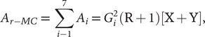 $$ {A}_{r- MC}\hskip0.3em =\hskip0.3em \sum \limits_{i-1}^7{A}_i\hskip0.3em =\hskip0.3em {G}_i^2\left(\mathrm{R}+1\right)\left[\mathrm{X}+\mathrm{Y}\right], $$
where Ci is the number of columns in which crop i is repeatedly planted in each row, and is uniformly 3 in our experiments, R is the number of rows in each plot, which is uniformly 21, and Gi is the spacing between each pair of plants, with the following conditions:
 $$ {\displaystyle \begin{array}{ll}{G}_i\hskip0.50em = 40\;\mathrm{cm},\;X = 2{C}_i,\;\mathrm{and}\;\;Y = 0,& \mathrm{for}\;i = BR,\\ {}{G}_i = 25\;\mathrm{cm},\;X = 0,\;\mathrm{and}\;\;Y = 1+{C}_i\left(S-1\right),& \mathrm{for}\;i\ne BR,\end{array}} $$
where S (= 6) is the number of non-BR species planted in each row. The derivation of equation (S4) is given in Supplementary Material S1.
The actual area (AA) of each replicate MC plot was calculated as:
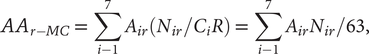 $$ {AA}_{r- MC}\hskip0.3em =\hskip0.3em \sum \limits_{i-1}^7{A}_{ir}\left({N}_{ir}/{C}_iR\right)\hskip0.3em =\hskip0.3em \sum \limits_{i-1}^7{A}_{ir}{N}_{ir}/63, $$
where Air is the land area for the ith crop in the replicate r, and Nir (≤63) is the number of surviving plants belonging to crop species i in the replicate r = 1, 2, …, 8.
2.4 Quantification of crop yield
The edible parts of each crop were harvested after maturity, and the quantity of the edible biomass harvested from each crop was separately weighed using a spring balance. The total crop harvest from each SC farm was weighed together, whereas the produce from the crops from each row and column from MC plots were separately weighed. As the fruits of brinjal and okra were harvested multiple times, the total weight of the fruits from each plant was estimated by successively adding their weights after each harvest (Deb, Reference Deb2021).
2.4.1 Yield per plant
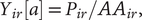
Considering the mortality of a few plants in different plots, we counted the number of surviving plants of each crop species in each farm plot, and estimated the per-plant productivity (Yir [p]) of crop i in the replicate plot r as
 $$ {Y}_{ir}\left[p\right]\hskip0.3em =\hskip0.3em {P}_{ir}/{N}_{ir}, $$
where Pir is the absolute yield of the ith crop in replicate r and Nir is the number of surviving plants belonging to crop species i in the replicate plot r.
2.4.2 Yield per unit area
Yield per unit area (Yir [a]) for crop i harvested from the replicate plot r was calculated by the standard procedure of dividing the absolute yield per unit area by the proportionate area in each plot:
 $$ {Y}_{ir}\left[a\right]\hskip0.3em =\hskip0.3em {P}_{ir}/{AA}_{ir}, $$
where AAir is the AA of the rth replicate plot under the ith crop and Pir is the absolute yield of the ith crop in replicate r.
To scale the yield of each SC plot at par with MC plots (with 63 plants), we calculated
 $$ {Y}_{ir- SC}\hskip0.3em =\hskip0.3em 63\;\left({P}_{ir- SC}/{N}_{ir- SC}\right), $$
where Pir is the absolute yield of the ith crop in the replicate plot r. The yield per unit area of each SP i in the replicated SC plots was then calculated as
 $$ {Y}_{ir- SC}\left[a\right]\hskip0.3em =\hskip0.3em {Y}_{ir- SC}/{A}_{r- MC} $$
with Ar−MC obtained from equation (S4). Equation (4b) thus enables a comparison between the yields of each crop from an equal area of SC and MC plots.
2.5 Indices of relative yield performance
2.5.1 Land equivalent ratio
Yield efficiency of MC with S = 7 crop species, compared to SC systems, was measured by LER (Mead & Willey, Reference Mead and Willey1980):
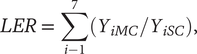 $$ LER\hskip0.3em =\hskip0.3em \sum \limits_{i-1}^7\left({Y}_{iMC}/{Y}_{iSC}\right), $$
where YiMC is the yield of the ith crop in the MC system (see equations (2) and (3) and YiSC is the yield of the same crop in SC plots. The total number of crop species planted to the poly-crop farm plots Σi = 7. An LER of >1 indicates that the amount of land required by the MC system is less than that of the SC farm to produce an equal yield. Conversely, an LER of <1 signifies more amount of land required for the MC farm to be as productive as the SC farm. Although LER is usually estimated using the yield of each crop per unit area, we made use of both Yir [a] and Yir [p] for each planting design.
2.5.2 Area time equivalent ratio
A more realistic comparison of the yield advantage of MC over SC considering the time duration of the component crops in the system, area time equivalent ratio (ATER; Aasim et al., Reference Aasim, Umer and Karim2008; Hiebsch & McCollum, Reference Hiebsch and McCollum1987), is calculated as
 $$ ATER\hskip0.3em =\hskip0.3em \sum \limits_{i-1}^7{ATER}_i, $$
 $$ {ATER}_i\hskip0.3em =\hskip0.3em \left({Y}_{iMC}/{Y}_{iSC}\right)\;\left({T}_i/{T}_L\right), $$
where Ti is the duration (in days) of the growth cycle of the ith crop species and TL is the duration of the species with the longest growth cycle. In our experiments, TL = 155 days.
2.5.3 Land use efficiency
The arithmetic average of LER and ATER is likely to give a more precise estimation of yield advantage than LER and ATER (Mason et al., Reference Mason, Leihner and Vorst1986):
 $$ LUE\hskip0.3em =\hskip0.3em \frac{\left( LER+ ATER\right)}{2}. $$
Originally put forward by Mason et al. (Reference Mason, Leihner and Vorst1986), equation (7) has been wrongly cited, and also corrupted by several authors. For instance, Yaseen et al. (Reference Yaseen, Singh and Ram2014) and Gitari et al. (Reference Gitari, Nyawade, Kamau, Karanja, Gachene, Raza, Maitra and Schulte-Geldermann2020) cited Mead and Willey (Reference Mead and Willey1980) as the progenitor of the formula, and also used a spurious formula for land use efficiency (LUE), which vitiated the results and interpretations of their experiments. Clearly, these authors and their peer reviewers had ignored to check up the cited works of Mason et al. (Reference Mason, Leihner and Vorst1986) and Mead and Willey (Reference Mead and Willey1980). Our present work intends to rectify these grave flaws.
3. Results and discussion
The data of edible biomass yield of each crop from all the SC and MC plots are given in (Deb, Reference Deb2021). The area and edible biomass yield per unit of land area (Y[a]) under each crop species from all plots are given in Supplementary Tables A1–A4. The data of edible biomass yield per plant (Y[p]) of all the crops are available in Table S1 of Deb (Reference Deb2021), and therefore not repeated here.
Figure 2 and Supplementary Tables A1–A3 show that the yield of each of the seven crops in MC farms is less than that of the same crops in SC plots. However, LER analyses reveal that the mean yields of the crops planted in mixed designs B and C are considerably greater than when the same crops are planted in either SC plots or in row intercropping (Design A), as discussed in detail in Deb (Reference Deb2021). The mean LER for the eight MC farms planted in Design B is 5.15, with a 95% confidence interval of (4.6, 5.7); the mean LER Design C is 5.67, with a 95% confidence interval of (5.0, 6.3).

Figure 2. Mean yield of crops in sole-crop and multi-crop farm plots. Vertical bars show standard deviations.
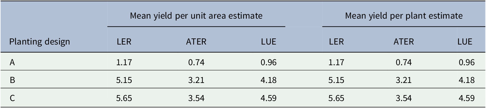
Here, we focus our analysis to estimations of yield and yield advantage indicators, and highlight that although the values of Yir [p] and Yir [a] are widely different, the values of LER using both Yir [p] and Yir [a] are identical (Table 1). While corroborating and expanding upon the findings of a large number of previous studies of MC systems compared to SC systems (e.g., the references cited in the Introduction section), our findings demonstrate for the first time that the value of LER remains invariant for both biomass per plant and biomass per unit area estimations. In fact, when Ai is identical in all the replicate plots (r = 1, 2, 3, …, 8), and the number of crop plants Ni in all the replicate plots is identical (Ni = Nir ), Yi [a] and Yi [p] are mutually derivable:
 $$ {Y}_i\left[p\right]\hskip0.3em =\hskip0.3em \left({A}_i/{N}_i\right)\;{Y}_i\left[a\right], $$
 $$ \mathrm{or},{Y}_i\left[a\right]\hskip0.3em =\hskip0.3em \frac{1}{\left({A}_i/{N}_i\right)}{Y}_i\left[p\right]. $$
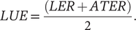
We denote the area per plant (Ai /Ni ) as the determining constant in the estimation of yield, so long as the intra- and interspecific spacings are kept invariant across all planting designs. Table 1 shows that LER remains invariant when calculated using both Y[a] and Y[p]. As a corollary, the values of ATER and LUE are also identical in both cases. Figure 3 illustrates the mean LER, ATER, and LUE for all three MC designs.
Figure 3. Mean LER, ATER, and LUE, invariant with Y[p] and Y[a] calculations of multi-crop plots with Designs A, B, and C. Vertical bars indicate standard deviations.
Because LER estimated using Yi [a] is no different from LER estimated using Yi [p], the value of ATER and that of LUE also remain invariant for both Y[a] and Y[p], as shown in Table 1 and Figure 3.
4. Conclusion
The primary results of this study are in conformity with previous, albeit limited, number of experimental productivity studies with mixed and polyculture systems, demonstrating that (a) overall crop yields of MC farms are decidedly superior to those of SC farms and (b) MC with row intercropping is scarcely more productive than monocultures (Deb, Reference Deb2021). This study also demonstrates that LER is a robust indicator of yield advantages, as it remains invariant whether estimated in terms of land area or the number of plants. ATER and LUE, derived from LER, are also robust, and truthfully depict the yield advantage of MC systems over SC systems.
Estimation of exact land area under a crop species in the MC farm plots is often a rigorous exercise, especially with complex crop planting designs with variable spacings between crop plants. Moreover, there is some scope of confusion in estimation of area, as some authors prefer to calculate the total land area in the MC plot, instead of the “occupied area” (e.g., X. Liu et al., Reference Liu, Rahman, Song, Yang, Su, Cui, Bu and Yang2018). In real-life situations, where indigenous farmers often randomly sow the seeds of diverse crop species with variable intercrop spacings in their MC farms, estimation of the land area is a tedious exercise. In such cases of difficulty in measuring yield per unit area (Yir [a]), yield per-plant (Yir [p]) estimation is much easier. Thus, LER, ATER, and LUE may safely be calculated using Yir [p], without compromising the exactitude of their values, as demonstrated in Table 1.
Table 1. Land equivalent ratio (LER), area time equivalent ratio (ATER), and land use efficiency (LUE) of multi-crop farms with seven crop species, planted in three different designs.
Supplementary Materials
To view supplementary material for this article, please visit http://doi.org/10.1017/exp.2021.33.
Data availability statement
All data are freely available on request.
Funding statement
Neither this work nor the authors received any financial support from any source.
Acknowledgments
We are grateful to Sachin Panigrahi for computer entry and formatting of all data. All logistic support to the field experiments was provided by Mr. Debjeet Sarangi of Living Farms, Bhubaneswar, who left our world during the preparation of this manuscript.
Conflicts of interest
The authors declare that there are no conflicts of interest.


 Open access
Comments
Comments to the Author: It is an excellently designed study. Add a few more recent references and discuss them in the text.