


1. Introduction
The net mass loss of the Antarctic ice sheet is estimated as ice mass discharged across grounding line, from which the surface mass balance (SMB) on the continent is subtracted. It is considered as the Antarctic ice sheet contribution to global sea-level rise (Rignot and others, Reference Rignot, Mouginot and Scheuchl2011a; Shepherd and others, Reference Shepherd2012; IMBIE, 2018). The majority of this excess discharge enters oceans through ice-shelf basal melting and iceberg calving (Hogg and others, Reference Hogg2017; Bell and Seroussi, Reference Bell and Seroussi2020). Ice flow velocity maps provide the rate at which ice is transported between different parts of the ice sheet, including mass transportation from the interior regions toward the ocean (Rignot and others, Reference Rignot, Mouginot and Scheuchl2011a; Gardner and others, Reference Gardner2018b). Accurate flow velocity maps are essential for studying the ice flow dynamics and mass balance of the Antarctic ice sheet (Rignot, Reference Rignot2006; Liu and others, Reference Liu, Wang, Tang and Jezek2012; Li and others, Reference Li2017; Gardner and others, Reference Gardner2018b).
There are many ice velocity products that are generated using remote-sensing data for individual glaciers, ice shelves and the entire Antarctic ice sheet. Synthetic aperture radar (SAR) and optical images are the main remote-sensing data for observing ice flow. However, in the context of this study, there are no SAR-based velocity maps in the 1960s–80s, mainly because the SAR satellite images were acquired only after the mid-1990s. Since then, a long record of SAR satellite images of European Remote Sensing satellite (ERS)-1/2, Radarsat-1/2, Envisat's Advanced Synthetic Aperture Radar, Advanced Land Observing Satellite-1's Phased Array type L-band Synthetic Aperture Radar and Sentinel-1 have been applied to map Antarctic ice flow velocities by using the interferometric SAR (InSAR) and offset tracking techniques (Rignot, Reference Rignot2006; Rignot and others, Reference Rignot, Mouginot and Scheuchl2011a; Mouginot and others, Reference Mouginot, Scheuchl and Rignot2012, Reference Mouginot, Rignot, Scheuchl and Millan2017a; Dirscherl and others, Reference Dirscherl, Dietz, Dech and Kuenzer2020). Despite its high precision, interferometric measurement of glacier velocities may be impossible if the imaged ice surface change exceeds half of the radar instrument wavelength, destroying the phase coherence between the two images. For example, this may occur in fast-flowing glaciers or regions with significant vertical deformation (Michel and Rignot, Reference Michel and Rignot1999). In these cases, the offset tracking technique that tracks speckles in the sequential SAR images is usually adopted as an alternative method (Joughin, Reference Joughin2002; Rignot, Reference Rignot2002; Scheiber and others, Reference Scheiber, Jager, Pratsiraola, De Zan and Geudtner2015).
A number of optical imaging satellite missions, including the Landsat series and the Moderate Resolution Imaging Spectroradiometer (MODIS), acquired remote-sensing data for ice velocity mapping in Antarctica. Ice surface features are extracted from optical images obtained at different times by feature tracking based on different matching algorithms (Heid and Kääb, Reference Heid and Kääb2012; Fahnestock and others, Reference Fahnestock2016), and the ice velocity can then be estimated through the tracked feature positions. Although the geometric precision of feature tracking in optical images is lower than that in SAR images, optical images have the advantage of significantly better coverage around the world in both space and time. An additional characteristic is their spectral signatures that can help identify unique features in Antarctica, such as blue ice (Hui and others, Reference Hui2014). Since the launch of Landsat-8 in 2013, its improved capability in both spatial resolution and spectral sensing has provided enhanced surface feature extraction in Antarctica, resulting in higher quality ice velocity products (Mouginot and others, Reference Mouginot, Rignot, Scheuchl and Millan2017a; Shen and others, Reference Shen2018; Gardner and others, Reference Gardner2018b).
Although many efforts were made to collect geodetic-quality measurements of ice velocity from in situ observations in the 1960s to later GPS-based dynamic monitoring (King, Reference King1994; Frezzotti and others, Reference Frezzotti, Capra and Vittuari1998; Bassis and others, Reference Bassis, Coleman, Fricker and Minster2005; King and others, Reference King, Coleman, Morgan and Hurd2007), as mentioned above, large-scale velocity mapping in Antarctica has been predominantly accomplished by satellite remote-sensing technology. However, compared to the recently acquired satellite data, early satellite observations have generally lower quality. For example, the Landsat images used in this study are from the Landsat program in the 1970s and 1980s, which are valuable but generally have lower image quality (e.g. stripes and low geolocation accuracy). They were only radiometrically calibrated and georeferenced through a systematic geometric correction using the spacecraft ephemeris data (USGS EROS, 2019). The data are supplied without georeferencing using ground control points (GCPs) and without terrain relief removal by orthorectification using digital terrain models. The geolocation error of these image data in Antarctica can be as large as 10 km, in addition to lower resolution, severe noises and stripe patterns in the images (Pan and Chang, Reference Pan and Chang1992; Tsai and Chen, Reference Tsai and Chen2008; Cheng and others, Reference Cheng2019). Consequently, the widely used ice velocity products at the regional or continental scales have been generated using data collected since the 1990s. On the other hand, a long record of the historical ice velocity is of great importance for both understanding the long-term evolution trend of the Antarctic ice sheet and predicting future global sea-level change (Payne and others, Reference Payne, Vieli, Shepherd, Wingham and Rignot2004; Rignot and others, Reference Rignot, Velicogna, Den Broeke, Monaghan and Lenaerts2011b; Shepherd and others, Reference Shepherd2012; IMBIE, 2018; Rignot and others, Reference Rignot2019).
From 1962 to 1963, KH-5 ARGON US reconnaissance satellites imaged the Antarctic ice sheet using photographic films during three missions (9034A, 9058A and 9059A) (Ruffner, Reference Ruffner1995; Wang and others, Reference Wang, Liu, Yu, Zhou and Cheng2016). The films showed significant deformation due to long-term storage before they were declassified and scanned in the 1990s (Galiatsatos, Reference Galiatsatos2009). Analytical photogrammetric models have been developed to handle film deformation, scanning errors, large-format lens distortion and block bundle adjustment (BA) issues for topographic mapping of the Arctic and Antarctic ice sheets (Zhou and others, Reference Zhou, Jezek, Wright, Rand and Granger2002; Kim, Reference Kim2004; Ye and others, Reference Ye2017). There are very limited numbers of ARGON stereo pairs in Antarctica for rigorous photogrammetric mapping of ice velocity from the 1960s (Li and others, Reference Li2017). The data selection for ice velocity mapping during the 1960s–80s in large glacier regions is thus focused on the combinations of ARGON (1960s)–Landsat (1970s–80s) and Landsat (1970s–80s)–Landsat (1970s–80s).
In addition to the difficulties in data processing and the defects inherent in the two datasets mentioned above, ice features for velocity estimation may not be tracked due to different appearances in the two datasets as well as physical changes in the ice surface over a period of 10–20 years. Furthermore, the traditional feature tracking methods suffer from difficulties in the trade-off between the search range and matching reliability, when applied to cases with a strong spatial variation in ice flow velocity (Liu and others, Reference Liu, Wang, Tang and Jezek2012; Li and others, Reference Li2017). If the search range is too large, the subsequent matching computation would be very intensive and may generate unreliable matching results. In contrast, if the search range is too small, the correct conjugate (corresponding) points could be missed, resulting in the failure of the matching. The hierarchical network-based image matching method was developed to address this problem by using a multi-layer image structure to control the search range by a coarse-to-fine scale and precise conjugate feature prediction to increase matching reliability and computational efficiency (Li and others, Reference Li, Hwangbo, Chen and Di2011; Liu and others, Reference Liu, Wang, Tang and Jezek2012). Efforts in using manually selected points in the initialization of the densification process were demonstrated to increase reliability (Li and others, Reference Li, Hwangbo, Chen and Di2011; Wang and others, Reference Wang, Liu, Yu, Zhou and Cheng2016). The method was further developed for simultaneous reconstruction of ice velocity fields and ice surface topography in Antarctica from stereo ARGON images of 1963 (Li and others, Reference Li2017).
Overall, due to the unavailability of high-quality remote-sensing data and difficulties in feature tracking methods, there is a lack of systematic ice velocity mapping from the 1960s–80s in basin-wide regions or all of Antarctica, although Li and others (Reference Li2017) produced an ice velocity map for 1963 of the Rayner Glacier using four photogrammetrically processed ARGON stereo images and Wang and others (Reference Wang, Liu, Yu, Zhou and Cheng2016) generated a partial ice velocity map for 1963–79 of the Larsen B Ice Shelf using ARGON (orthorectified) and Landsat Multispectral Scanner (MSS) images.
The objective of this paper is to improve the methodology for systematic ice velocity mapping of Antarctica using the ARGON and Landsat images from the 1960s–80s. Our new historical velocity mapping framework uses an enhanced hierarchical network densification method to meet additional challenges, including heterogeneous image qualities of ARGON and early Landsat images, extremely diverse range of ice flow dynamics and disappearance of ice surface features after a long time-span of over 10 years. The method has been applied to a study area covering the Jutulstraumen Glacier, Fimbul Ice Shelf, Schytt Glacier, and Jelbart Ice Shelf. The produced historical ice velocity maps are compared with recent ice velocity products to characterize the ice dynamics. Finally, the maps are utilized to estimate the mass changes in the area during the early years, which provides important information for the long-term mass-balance study of Antarctica.
2. Study area and data
The Fimbul and Jelbart ice shelves are the two largest ice shelves along the northeastern Weddell Sea in Queen Maud Land (QML), East Antarctica (Fig. 1). The area of the two ice shelves is 63 347 km2, and is representative of medium-sized and mid-latitude ice shelves in Antarctica (Griggs and Bamber, Reference Griggs and Bamber2011). The Fimbul Ice Shelf is fed by the fast-flowing Jutulstraumen Glacier, which is responsible for ~10% of ice discharge from the QML sector of the Antarctic ice sheet (Langley and others, Reference Langley2014). The Jelbart Ice Shelf is fed by the Schytt Glacier, which is narrower than the Jutulstraumen Glacier (Goel and others, Reference Goel, Brown and Matsuoka2017).
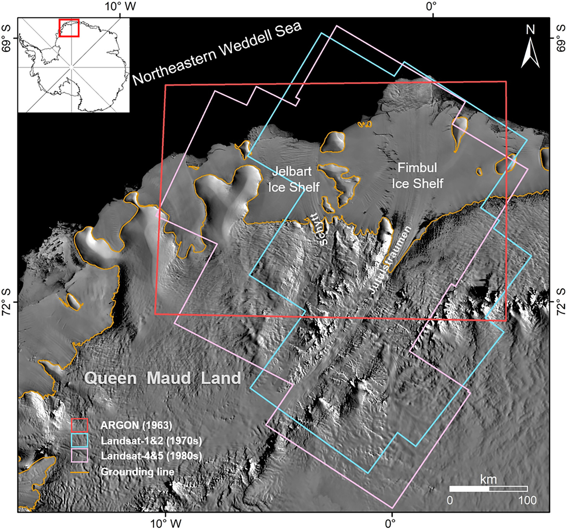
Fig. 1. Study area of the Fimbul and Jelbart ice shelves in QML with footprints of the satellite images, MOA mosaic 2004 as the background (Haran and others, Reference Haran, Bohlander, Scambos, Painter and Fahnestock2005) and grounding line from Gardner and others (Reference Gardner2018a).
The ice velocity in recent years (1997–2017) in the study area can be described by three ice velocity products. The earliest is the ice velocity map derived by tracking features between the Antarctic Mapping Mission (AMM-1) mosaic of September–October 1997 and the Modified Antarctic Mapping Mission (MAMM) mosaic of the fall of 2000 (Jezek, Reference Jezek2002). The second product is the surface velocity map generated by applying the InSAR technique using multisource SAR satellite data obtained between 2007 and 2009 (Rignot and others, Reference Rignot, Mouginot and Scheuchl2011a; Mouginot and others, Reference Mouginot, Scheuchl and Rignot2017b). The latest product consists of several annual maps in the 2013–17 period constructed from Landsat-8 images (Fahnestock and others, Reference Fahnestock2016; Shen and others, Reference Shen2018; Scambos and others, Reference Scambos, Fahnestock, Moon, Gardner and Klinger2019). An ice flow center line runs from the glacier main trunk to shelf front and describes the pass of ice mass from the glacier feeding the ice shelf. Based on the InSAR ice velocity map from 2007–08 (Mouginot and others, Reference Mouginot, Scheuchl and Rignot2017b), the ice flow velocity along the ice flow center line of the Jutulstraumen Glacier and Fimbul Ice Shelf is ~710 m a−1 at the grounding line and ~750 m a−1 at the shelf front. Similarly, the ice flow velocity of the Schytt Glacier and Jelbart Ice Shelf is ~370 m a−1 at the grounding line and ~610 m a−1 at the shelf front. In this paper we use the terms of velocity and speed interchangeably for simplicity and consistency.
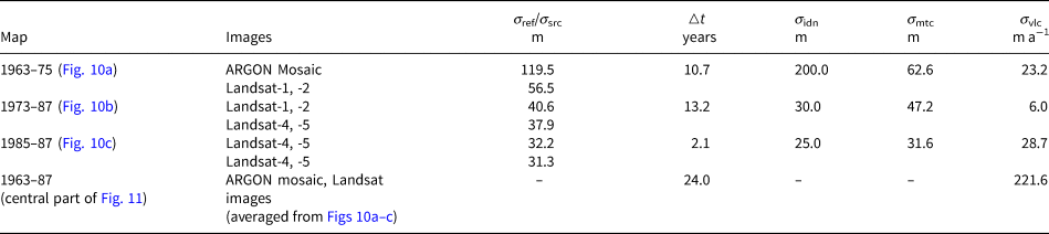
The available satellite images from the 1963–89 covering the Fimbul and Jelbart ice shelves were selected to reconstruct the early ice velocity history in the study area. The selection considerations included low coverage of clouds, overlapping of two or more images in the mapping period and the existence of stable landmarks serving as controls for orthorectification. Subsequently, 77 images or products covering three decades were chosen (Table 1 and Table 6), namely, (1) ARGON images from 1963 presented as an orthorectified mosaic product (Kim, Reference Kim2004), (2) Landsat-1 and -2 images from the 1970s and (3) Landsat-4 and -5 images from the 1980s. The Landsat images are of the processing level L1GS which were radiometrically calibrated and required further geometric rectification before they could be used for ice velocity mapping. The data were downloaded from the USGS Landsat distribution site (https://earthexplorer.usgs.gov/). The near-infrared band of Landsat images is used for velocity computation (band 7 of the MSS sensor and band 4 of the TM sensor). For the geometric control of these selected satellite images, the Landsat image mosaic of Antarctica (LIMA), a higher resolution (15 m) digital mosaic produced from nearly 1100 Landsat-7 ETM+ images collected between 1999 and 2003 (Bindschadler and others, Reference Bindschadler2008), was used as the horizontal reference; and the earliest Antarctic DEM product Radarsat Antarctic Mapping Project (RAMP) Digital Elevation Model (DEM) Version 2 (RAMPv2) served as the elevation reference (Liu and others, Reference Liu, Jezek, Li and Zhao2015). RAMPv2 synthesized elevation data originating from ERS-1 altimetry observations and survey data from the 1940s to 1990s, which is close to 1963–89, the time span of the historical images for velocity mapping in this study. Therefore, this justifies the selection of RAMPv2 for the use as vertical control data over the recently available Antarctic DEM, reference elevation model of Antarctica (REMA) of 2009–17 (Howat and others, Reference Howat, Porter, Smith, Noh and Morin2019), despite of its higher resolution and accuracy.
Table 1. Summary of the historical remote-sensing images and products used in this paper
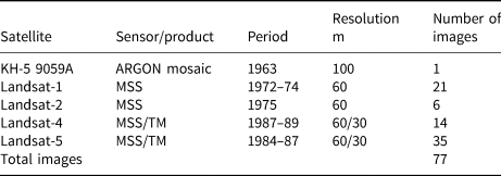
See Table 6 for detailed image information.
3. Method
The proposed framework for the systematic ice velocity mapping of Antarctica using historical images consists of three modules, historical Antarctic image orthorectification, historical velocity field construction and final velocity map generation (Fig. 2). Challenges stemming from both historical image processing and the unique Antarctic environment are addressed by developing new techniques. The Landsat images of 1972–89 are orthorectified using GCPs measured on the RAMPv2 DEM and LIMA image mosaic to provide, along with ARGON Mosaic of 1963, orthorectified historical images for velocity mapping. The key module is hierarchical network densification through a multi-layer recursive matching and tracking approach to build velocity vectors of the ice velocity field. This method overcomes difficulties faced by a single-layer matching technique in cases of significant spatial variations of displacements in a stereo image pair (e.g. cliff areas in terrain mapping or fast flowing glaciers in velocity mapping). The methodology was successfully applied in terrain surface reconstruction in urban areas (Rothermel and others, Reference Rothermel, Wenzel, Fritsch and Haala2012) and planetary landing site topographic mapping (Li and others, Reference Li, Hwangbo, Chen and Di2011). It was implemented to estimate Antarctic ice flow velocities (Liu and others, Reference Liu, Wang, Tang and Jezek2012; Li and others, Reference Li2017) and further extended here for systematic reconstruction of basin-wide ice flow velocity fields. A set of manually selected seed points on the initial layer supplies the structural velocity information ranging from the slow ice flow in the inland interior to the rapid motion at the ice-shelf front. Guided by the seed points and increasingly densified feature points in a triangulated irregular network (TIN) model, the recursive feature matching and tracking are carried out layer-by-layer where an adaptive search range is determined according to the velocity information in the existing TIN model. This ensures the reliability of the matched ice surface features through high-quality candidates and increased computational effectiveness by using reduced search ranges. The matched feature points are further filtered to eliminate outliers and then used to control the dense grid matching process to produce the final multi-temporal velocity maps, which can be used for various Antarctic applications.
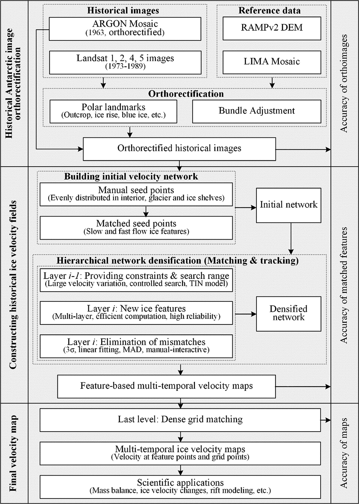
Fig. 2. Framework for systematic ice velocity mapping of Antarctica using historical images, with three modules (historical Antarctic image orthorectification, constructing historical velocity fields and final velocity map) and detailed processing steps and methods. Accuracies of the components evaluated in the first two modules are used to estimate the accuracy of final maps in the last module using Eqn (1).
3.1 Historical Antarctic image orthorectification
The first module of the framework (Fig. 2) is used to prepare the ARGON mosaic from 1963 and Landsat-1, -2, -4 and -5 images from the 1970s and the 1980s in the form of orthorectified images. The individual processing steps include image preprocessing, selection of GCPs, BA and orthorectification (McGlone, Reference McGlone2004). The datasets for the three maps are reprojected as orthorectified images of different decades in a single vertical and horizontal reference frame (WGS 84 and Antarctic Polar Stereographic projection EPSG 3031). Through these processing steps, the geometric imaging geometry differences, film distortion, cartographic projection differences and geolocation errors can be eliminated or significantly reduced (McGlone, Reference McGlone2004). More specifically, the ARGON mosaic of Antarctica (MOA) used in this study is already an orthorectified mosaic. The original ARGON images are processed using a rigorous photogrammetric model, BA, to estimate the interior and exterior orientation parameters of the images (Kim, Reference Kim2004; Sohn and others, Reference Sohn, Kim and Yom2004). The BA process requires a set of GCPs for linking to the reference frame and a set of tie points for connecting the images. The estimated interior and exterior orientation parameters and a DEM are then used to produce the orthorectified ARGON image (Schenk, Reference Schenk1999; McGlone, Reference McGlone2004; Li and others, Reference Li, Hwangbo, Chen and Di2011). To orthorectify Landsat-1, -2, -4 and -5 images, we select a set of GCPs that appear in both the Landsat images of an image pair and the reference data that includes the LIMA image mosaic and RAMPv2 DEM. There are very few GCPs surveyed in Antarctica by GPS due to the remote and hostile environment. To address this problem, unique landmarks on the Antarctic ice sheet, which are stationary or whose motion is negligible, including outcrops, blue ice features, ice rises and others, should be used for georeferencing.
Rock outcrops are considered the most stable landmarks for GCPs, although they may be partially or completely covered by seasonal accumulations. Their initial locations can be identified with the help of the Antarctic Digital Database (Burton-Johnson and others, Reference Burton-Johnson, Black, Fretwell and Kaluza-Gilbert2016; ADD, 2021), which provides the distribution of rock areas in Antarctica. The precise positions of the GCPs are determined in three steps. Assume that an outcrop protrudes from the ice surface, the first step is to identify the outcrop top through a shading examination. For example, given the solar altitude angles (α al) and azimuth angles (α az) of the two historical images, the same outcrop top can be distinguished from rock shadows, which may appear differently in the images (Figs 3a, b). Mistakes are often introduced by choosing shadow corners in two images, which may appear similar, but are cast from different features. In the second step, considering the detailed topographic information provided by its high-resolution gridpoints, the REMA DEM is used to generate two synthetic shaded relief maps using the same solar illumination geometry as at the respective image acquisition times (Figs 3c, d). The identified outcrop top in the first step can be checked against these shaded relief maps or those produced with different (artificial) illumination geometry to ensure the same outcrop is matched in two images. In the third step, a set of 3-D views of the outcrop can be built by draping the historical images and shaded relief maps on the REMA DEM for the final verification (Figs 3e, f). This complex procedure is currently performed manually and requires automation in the future.
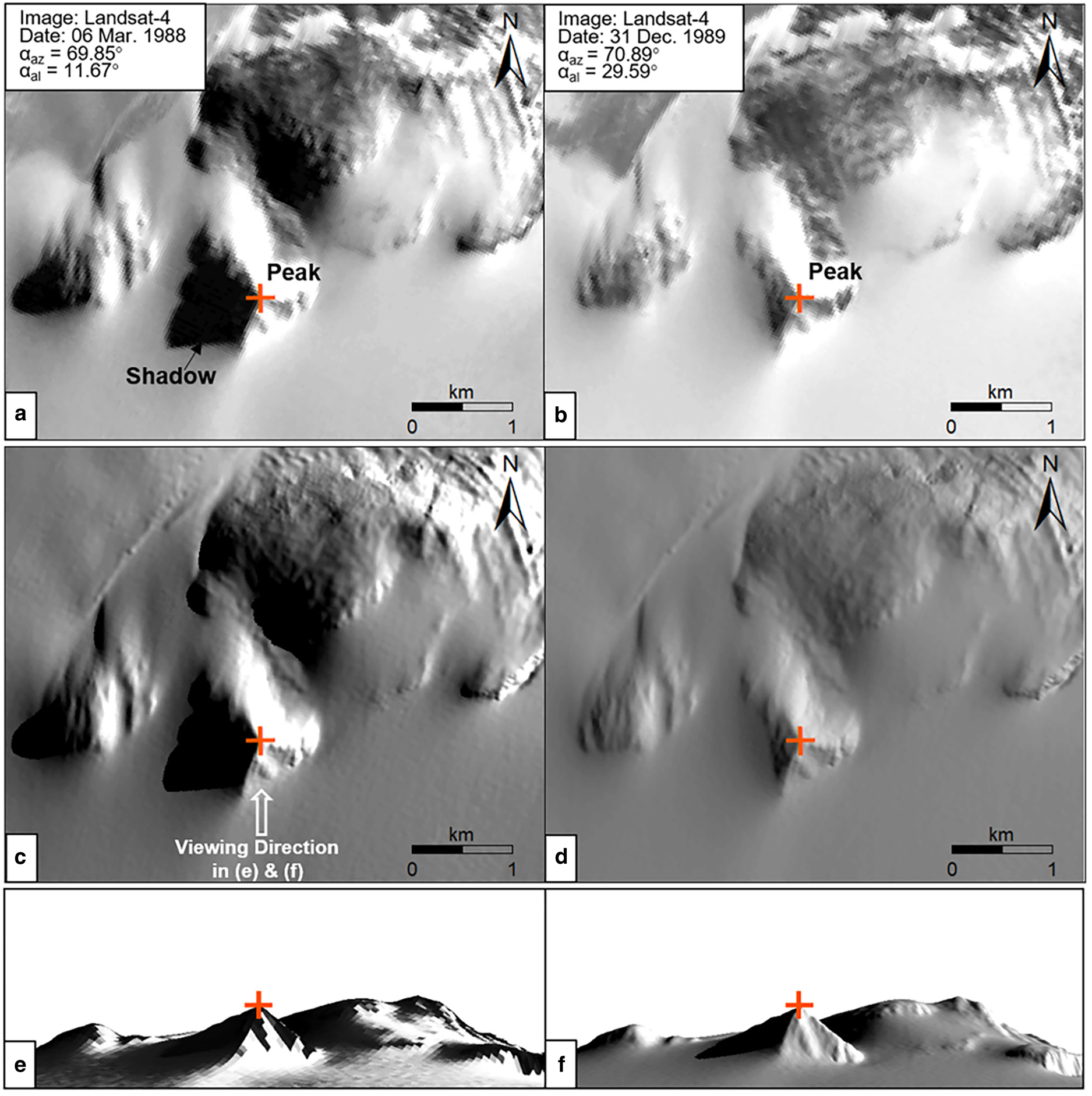
Fig. 3. Example of verification of an outcrop top as GCP: (a) and (b) are two Landsat-4 images from which the outcrop top is selected by distinguishing different shadows caused by varying solar altitude and azimuth angles; (c) and (d) are two shaded relief maps from the REMA DEM using the same solar illumination geometry at the image acquisition time; (e) and (f) are two 3-D views of Landsat-4 in (a) and the shaded relief map in (c) (the elevation is exaggerated by two times), respectively.
Blue ice areas in Antarctica may not be covered by snow due to wind and topography, and the ice appears blue, relatively smooth, and flat. In areas where the surface is covered by ice, and no outcrops are available, blue ice landmarks are often used as GCPs. Blue ice is formed when ice bubbles are squeezed out of ice over time, and the ice density increases, strengthening the ice surface and improving the surface hardness (Bintanja, Reference Bintanja1999; Cui and others, Reference Cui2019). The blue ice features with relatively low velocities that may move at <1 m a−1 occupy ~37% of the blue ice areas in Antarctica (Hui and others, Reference Hui2014). We use a dataset of blue ice features with location information in Antarctica provided by Hui and others (Reference Hui2014). Given the initial location of a blue ice GCP candidate from the dataset (Fig. 4a), we examine the velocity within a relatively long period to confirm the locational stability. We require the velocity of the candidate area to be <10 m a−1 (or within map uncertainties) in two different velocity maps (Fig. 4c). The time separation of the two maps is more than 8 years, e.g. the MAMM velocity map from 1997/2000 (Jezek, Reference Jezek2002) and InSAR velocity map from 2007–08 (Mouginot and others, Reference Mouginot, Scheuchl and Rignot2017b). To further avoid or reduce the influence of seasonal snow cover and outline changes of the blue ice area, we make measurements at higher and distinct locations within the blue ice area with the help of illumination and shadow interpretation in images or 3-D scene analysis using a DEM, if available (similar to Fig. 3).
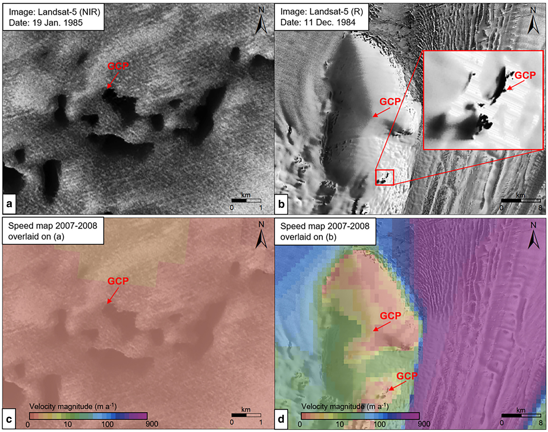
Fig. 4. Examples of landmarks used as GCPs: (a) blue ice shown in a near infrared band image of Landsat-5; (b) outcrop (in inset) and peak formed by an ice ridge intersection on ice rise in a red band image of Landsat-5; (c) and (d) InSAR velocity map of 2007–08 (Mouginot and others, Reference Mouginot, Scheuchl and Rignot2017b) overlaid on (a) and (b), respectively.
In addition, ice rises are common, locally grounded features in ice shelves. They often have a dome-shaped surface that is 100–200 m higher than the surrounding ice shelf. GCPs can be selected from ice rise landmarks that usually remain stable long-term and are not overrun by the ice sheet, at least during the last glacial cycle (Matsuoka and others, Reference Matsuoka2015). However, the surface of an ice rise is usually covered with snow and ice and may be subject to seasonal snow changes. First, because stable landmarks are generally less available in ice-shelf regions, outcrops on ice rises should also be selected as GCPs (Fig. 4b). Second, peaks formed by sharp ice ridge intersections at high locations are relatively stable and should be selected as GCPs because they are less affected by snow accumulation (Fig. 4b). Lower areas with ice flow or migration of shear margins are not considered. One or more high-precision velocity maps, such as the InSAR velocity map of 2007–08 (Mouginot and others, Reference Mouginot, Scheuchl and Rignot2017b), may be used to check the decadal-scale stability of the selected GCPs (Fig. 4d). Therefore, stationary features on ice rises can be used as GCPs, as suggested by Wang and others (Reference Wang, Liu, Yu, Zhou and Cheng2016).
In general, the principle is to select enough GCPs that are evenly distributed in the image to be orthorectified. In areas where the three types of landmarks are not available, other distinct image features with very slow motion (<10 m a−1) may also be selected as GCPs (Li and others, Reference Li2017).
With the selected GCPs measured on the historical image for image coordinates, the LIMA image mosaic for horizontal control and the RAMPv2 for vertical control, an orthorectification model that is described by Toutin (Reference Toutin2004) and implemented in the PCI Geomatica system (Geomatics, 2005) is used to produce an orthorectified historical image for subsequent ice velocity mapping.
3.2 Construction of historical ice velocity fields
After the orthorectification process, both the orthorectified ARGON mosaic and Landsat images are free of distortion caused by terrain relief (Li, Reference Li1998). Tracing the same ice surface features on the two images produces a motion displacement map that describes the motion vectors of the ice velocity field. Therefore, the second module of the framework (Fig. 2) focuses on the construction of basin-scale historical ice velocity fields through a dynamically densifying motion vector network approach that is modified from our in-house hierarchical image matching system that was successfully applied for surface feature tracking in challenging polar environments (Li and others, Reference Li2017). One of the main advantages of this hierarchical image matching strategy is its capability in estimating adaptive search ranges for accommodating large velocity variations while maintaining a high level of reliability by obtaining high-quality matched points and avoiding mismatches; the computational efficiency is achieved by its reduced search range on each scale level and the coarse-to-fine multi-scale matching strategy.
Initialization: To estimate the velocity of an ice surface feature, the identified feature in the earlier image (reference image) must be uniquely tracked in the later image (search image). The first difficulty for an automatic tracking process in an Antarctic scene is attributed to the lack of distinct textures, which most general tracking techniques rely on. In the second difficulty, velocity in a scene, thus, displacements between features in two images may vary dramatically or discontinuously. For example, the velocity of a fast-flowing glacier may increase from a very low velocity (<10 m a−1) in the inland interior to a high velocity (more than 800 m a−1) at the ice-shelf front; furthermore, the velocity outside the shear margin of the fast-flowing main trunk may be relatively low. This makes it extremely difficult to determine the search range in the feature matching process. The third difficulty is that persistent surface features may not have been preserved over the long-time intervals of the historical images because of the Antarctic dynamic surface processes, such as snow accumulation and blowing snow. In this study, the hierarchical feature tracking approach builds a pyramid of multilevel velocity fields, where the aggregated large surface structures are matched on the top level and used to control the subsequent lower level, leading to more expanded persistent features in a recursive manner. In the present experimental results, automated image matching techniques, both areal and feature-based matching, tend to find slow motion or stable ice features on the top level. Therefore, we start with a set of seed points that are manually selected and matched in two images (Wang and others, Reference Wang, Liu, Yu, Zhou and Cheng2016; Li and others, Reference Li2017), which may include surface features in slow-flowing areas, such as those used as GCPs, for example, outcrops, blue ice and ice rises. Additional seed points are selected on high-velocity features such as surface undulations and fractures on glaciers and ice shelves (Fig. 5a). Such manually selected seed points are highly effective for handling images with a time interval of more than 3 years. Another example of features used for seed points is rifts that appear frequently near ice-shelf fronts. They may have evolved (widening and lengthening) from upstream fractures, showing different longitudinal velocities on the two sides of the rifts (Hulbe and others, Reference Hulbe, Ledoux and Cruikshank2010; Walker and others, Reference Walker, Bassis, Fricker and Czerwinski2013). The transverse rifts may meet flowlines at an angle; and tips of promontories formed by rift walls can be identified with the help of 3-D visualization, if possible, and used as seed points (Fig. 5b).
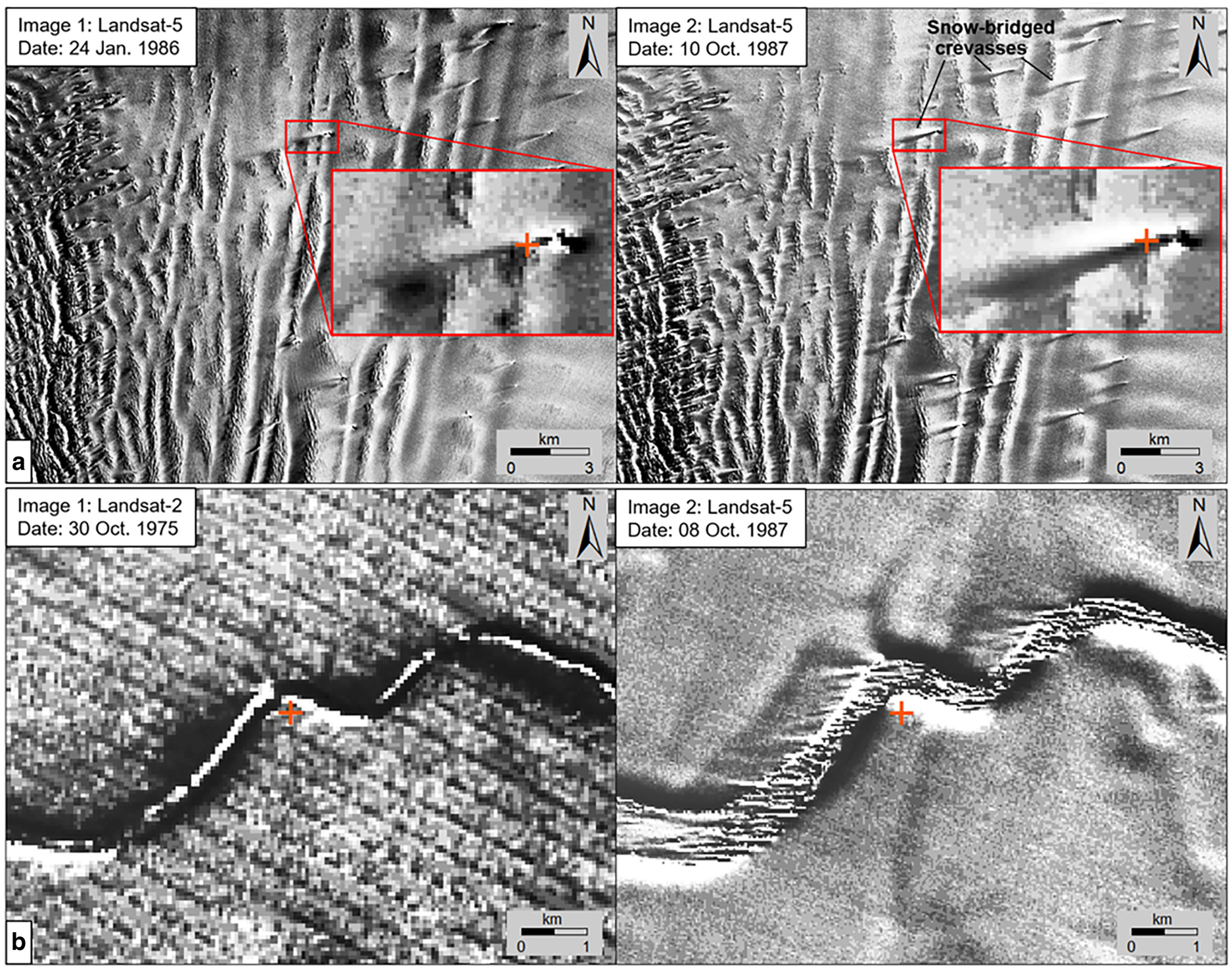
Fig. 5. Selection and matching of seed points from large structural features on an image pair: (a) intersections of crevasses (snow-bridged) and ice flow features on a glacier; (b) tips of promontories formed by rift walls on an ice shelf.
The distribution of different types of seed points in the area covering the Fimbul and Jelbart ice shelves is shown in Figure 6. A total of 1087 seed points are selected manually to provide structural information of the velocity field on the top level. The initial TIN model uses large-scale (a few kilometers to tens of kilometers) ice surface structure features (outcrops, blue ice, ice rise and others) and slow velocity surface features (<10 m a−1) to form a network that is used to constrain the stationary and slow-flowing part of the velocity field. Furthermore, at a smaller scale (hundreds of meters to a few kilometers) ice surface features in fast-flowing regions, such as main trunks of glaciers and ice shelves, are used to guide the densification process of the fast-flowing part of the velocity field.
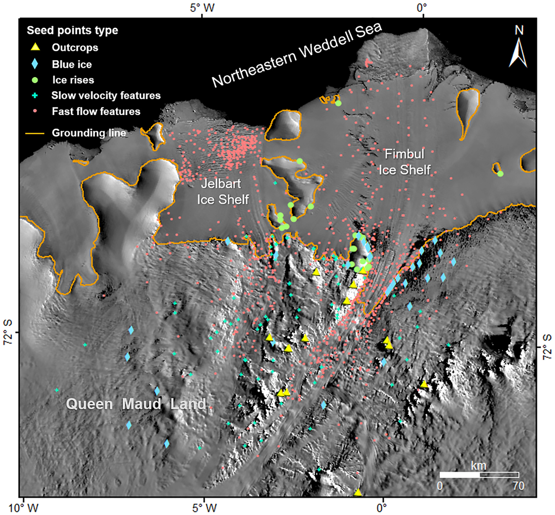
Fig. 6. Distribution of different types of seed points selected in the area covering the Fimbul and Jelbart ice shelves and the corresponding drainage basin. The grounding line is from Gardner and others (Reference Gardner2018a). The background image is MOA mosaic 2004 (Haran and others, Reference Haran, Bohlander, Scambos, Painter and Fahnestock2005).
Hierarchical network densification: Given an image with a dimension of M 1 pixels × M 2 pixels, an N-layer network has a dimension structure of M 1/2N −i × M 2/2N −i at the i-th layer (i = 1, 2, …, N), with the first layer of the coarsest image and the N-th layer of the original image (Fig. 7). In this study, we implement a network of a four-layer image pyramid which is generated through a top-down (from N-th to 1st layers) procedure. Images at each layer are generated using a Gaussian filter that simultaneously subsamples and smooths the images from the previous layer (Li and others, Reference Li, Hwangbo, Chen and Di2011).
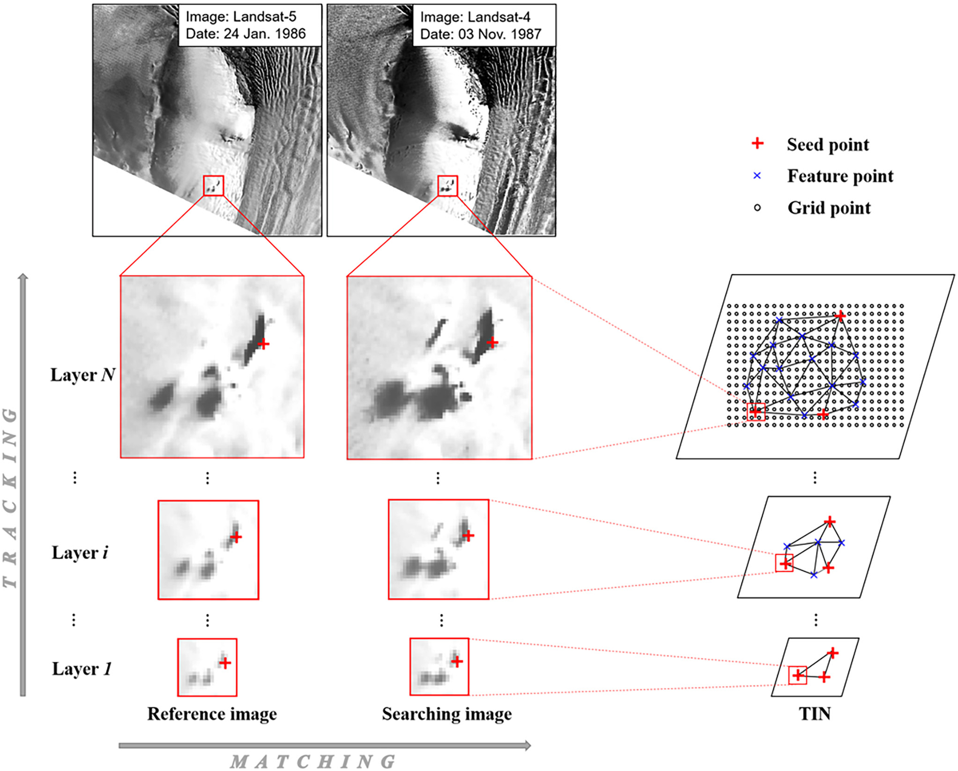
Fig. 7. Schematic diagram of the hierarchical network densification approach. The method is applied to the entire image pair. An enlarged area is used to explain the hierarchical matching and tracking process.
The hierarchical ice velocity network is densified recursively by two processes, namely matching ice surface feature points from the reference image to the search image and tracking the matched features from the current layer to next layer (Fig. 7). Initially, a set of seed points (red crosses) is selected and matched manually on the top layer (layer 1) to construct the initial structural information of the velocity field. At each layer (layer i), the tracked feature points from the previous layer (layer i − 1) are used to form triangles of a TIN model on this layer. New feature points are then detected in both images using a Shi–Tomasi corner detector (Shi and Tomasi, Reference Shi and Tomasi1994; Tulpan and others, Reference Tulpan, Belacel, Famili and Ellis2014). For each feature point on the reference image its adaptive search range is adjusted by the velocity information inherited in the TIN model (Li and others, Reference Li2017). Its corresponding feature point on the search image is found from a set of candidate feature points in the search range by using the area-based matching technique. After feature matching and outlier elimination are performed at all feature points, the matched feature points are passed on to the next layer (layer i + 1), where they are verified by an area-based feature tracking method. The tracking process includes an area-based matching between the feature point on layer i and its transformed point on layer i + 1. Then the tracked feature point is rematched on layer i + 1 between the reference and search images using detailed image information of a higher resolution. The remaining feature points after this tracking process are used to densify the TIN model. On the last layer (layer N), under the control of the TIN model, a dense grid mapping is performed at a grid spacing of 10 pixels through a subpixel matching process using normalized correlation coefficients (NCCs; Liu and others, Reference Liu, Wang, Tang and Jezek2012).
There are two additional techniques for eliminating mismatches and feature points of erroneous velocities at each level. The first uses a multi-thresholding technique of correlation coefficients to avoid mismatches caused by areas of different ice flow patterns. Among other factors, the correlation coefficients of the corresponding feature points are closely related to the quality of the image pairs involved. Generally, a mapped area in historical images may appear as a large, low-contrast and low-textured background with slow ice flow, where one or more fast-flowing glaciers may emerge (Fig. 8a), resulting in a bimodal histogram of the correlation coefficients (Fig. 8b). Experiments with manual measurements show that correct matches of slow ice flow features exist within the first peak area of the relatively low correlation coefficients, while features with higher velocity are more distinct and thus have higher correlation coefficients and are less affected by the low-image quality (Heid and Kääb, Reference Heid and Kääb2012; Li and others, Reference Li2017). Therefore, we separate the two groups of automatically matched feature points using the threshold between the bimodal distributions at each level and then determine the selected feature points within each group using a different threshold. This two-level thresholding process not only ensures that reliable feature points of both slow and fast flows are matched, but also that mismatches caused by a single threshold are avoided.
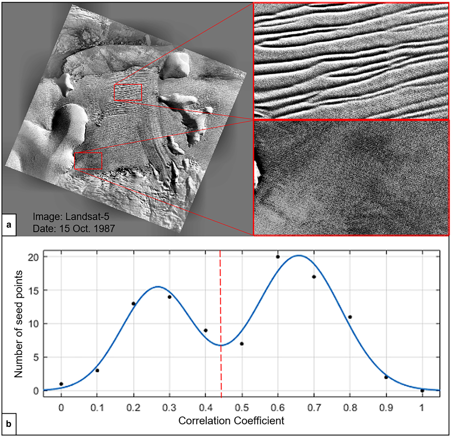
Fig. 8. Thresholding technique for eliminating mismatches: (a) historical scene with a large low contrast and low textured background and a fast-flowing glacier with corresponding enlarged areas; (b) bimodal histogram of correlation coefficients.
The second technique used for eliminating erroneous ice velocity vectors that are produced from the remaining mismatches is based on the knowledge that the ice velocity of a glacier must follow glaciological processes and generally does not abruptly change its magnitude and direction within a close neighborhood. Initially, we use a threshold based on the estimated error of the ice velocity map (e.g. 1–2 times) to remove ice flow vectors in the motionless or slowly moving areas to avoid the chaotic appearance. Then a velocity vector in a faster flowing area is considered abnormal and eliminated if its magnitude difference with the local mean is more than three times the std dev. In addition, the consistency of the flow direction of the velocity vectors is strongly correlated with the ice velocity. The velocity vectors in a small neighborhood may change their directions significantly only in low-velocity areas or even show a chaotic pattern because of the matching errors. Therefore, we perform a rule-based process to eliminate velocity vectors with erroneous directions. First, we prescreen each velocity direction α against an existing ice velocity map, for example, the InSAR velocity map by Mouginot and others (Reference Mouginot, Scheuchl and Rignot2017b). If the difference dα is greater than a threshold δ (dα ≥ δ), the velocity vector is considered erroneous and should be eliminated; δ is set sufficiently large to prescreen blunders by using a set of descending values (δi for velocity rangei): 90° for 10–20 m a−1, 70° for 20–50 m a−1, 60° for 50–100 m a−1, 52° for 100–200 m a−1, 46° for 200–400 m a−1 and 40° for ≥400 m a−1, which are estimated through a number of experiments with manual measurements. Then, the remaining velocity vectors are checked for internal consistency. For each feature with ice velocity in the range of 10–20 m a−1, we check its consistency with a mean and std dev. (1σ) calculated within a neighborhood (5 km is used in this paper) based on the trial result of several areas. For a feature with a velocity ≥20 m a−1, the maximum angular difference within the neighborhood must be <30°. Otherwise, the feature is checked against the median absolute deviation estimated within the neighborhood (Liu and others, Reference Liu, Wang, Tang and Jezek2012) and is accepted with a quantile of 90%. For those that have fewer than three feature points within the neighborhood, a manual check is performed (MPAISSIVP, 2019).
Overall, the hierarchical ice velocity network densification process is initiated with a set of reliable manual seed points to present the structural features at the first level. The subsequent recursive network densification process is characterized by two main steps: (1) improved reliability and efficiency by producing high-quality matches and avoiding mismatches through inherited constraints and search ranges using tracked feature points from the previous level, and (2) elimination or reduction of remaining erroneous velocity vectors using a rigorous rule-based procedure.
3.3 Final ice velocity maps and accuracy assessment
The final ice velocity maps defined in a grid are generated using the relatively sparsely distributed feature points achieved through hierarchical network densification as a control; velocities at the densely distributed gridpoints are then estimated by displacements calculated using the dense grid matching technique (Fig. 2). The algorithms of NCC matching, geometric constraints and search range adaptation are implemented in a similar manner in both dense grid matching and hierarchical network densification. The grid spacing is generally selected as 1.5–3 times the lowest ground resolution of all images involved (Li, Reference Li1998). The grid spacing can also be estimated from the ratio of the mapping area to the number of matched feature points. However, the matched feature points spread more sparsely in some locations, and there may be unmatched blank areas due to the poor quality of the historical images and long-term glaciological processes. For applications that require high-accuracy velocities, large areas (e.g. >12 km2) without mapped velocity points are masked out. In this product, the ice velocity is split into its components in the x and y directions at each gridpoint, from which the magnitude and direction are calculated and/or stored in the dataset.
Figure 9 illustrates the effectiveness of the proposed method. Figure 9b presents the velocity map of the main trunk of the Jutulstraumen Glacier produced through the hierarchical network densification procedure using the seed points in Figure 6. In comparison, Figure 9c illustrates the result of a single layer area-based matching technique without seed points. The high velocity variation of the area makes it impossible to use a fixed search window size that would work with both the very slow-moving ice surface (<10 m a−1) and high-velocity ice flow (>800 m a−1) at the ice-shelf front. Without the guidance of the seed points in the TIN network (Fig. 9a), a larger search window caused many mismatched feature points that failed to map the very low-velocity areas (<10 m a−1), in addition to the increased computational cost (Fig. 9c). Similarly, mismatches along the high velocity main trunk are also obvious. Velocity maps with such large errors would influence the scientific conclusions.
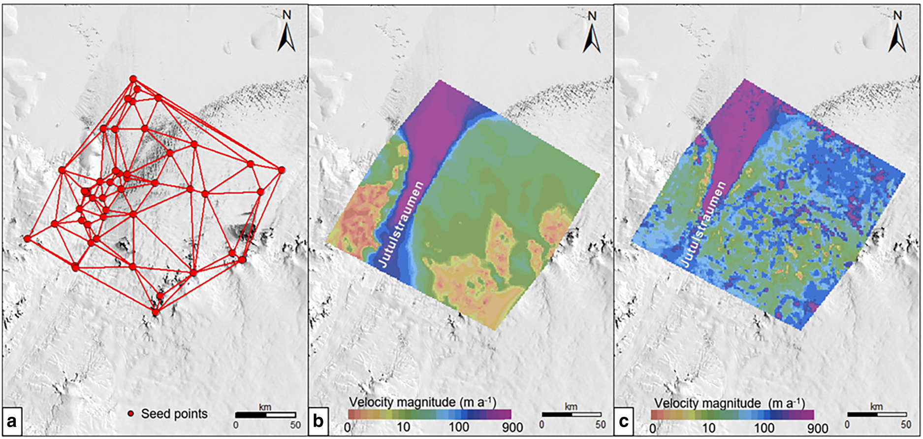
Fig. 9. Impact of the proposed method on historical ice velocity mapping in the main trunk of the Jutulstraumen Glacier: (a) initial network generated based on the seed points, (b) improved velocity map produced using the hierarchical network densification approach supported by the seed points and (c) undesirable result of single layer matching without seed points.
In this study, we use σ ref and σ src to denote the geolocation uncertainties of the reference and search orthoimages. Because the final velocity maps contain both matched feature and gridpoints at the last layer of the densified network, an identification accuracy σ idn for localizing a feature in the reference orthoimage is used for feature points (σ idn = 0 for gridpoints). Here, it is set to 0.5 pixels for Landsat images and, 2 pixels for ARGON images. The accuracy is further influenced by the matching accuracy σ mtc. Assuming that the time span between two images is Δt and the errors involved are independent, the ice flow velocity error σ vlc can be estimated as
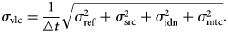
In principle, the orthorectification errors of σ ref and σ src consist of the error of the Landsat images and the errors introduced from LIMA and dominantly from RAMPv2 through the rectification process. In practice, we evaluate the orthorectification accuracy by comparing the horizontal locations of a set of checkpoints which are measured manually in the LIMA image mosaic and the orthoimages produced in the PCI Geomatica system (Toutin, Reference Toutin2004; Geomatics PCI, 2005). Displacements calculated on stable terrain, such as outcrops in the ADD database (Burton-Johnson and others, Reference Burton-Johnson, Black, Fretwell and Kaluza-Gilbert2016; ADD, 2021), represent errors. We select up to ten checkpoints that are evenly distributed in slow-flowing areas (outcrops or points with velocity ≤10 m a−1). The displacements between the locations of the checkpoints in the LIMA image and the orthoimages represent residual errors after the orthorectification process. The RMSE from the displacements is used to estimate the orthorectification uncertainties σ ref and σ src. Similarly, the image matching error σ mtc can be estimated using the differences between the automatically matched and manually matched locations of a set of checkpoints. We divide the map into a checking grid and select one or more checkpoints (matched points) in each gridcell to ensure a uniform distribution (Li and others, Reference Li, Hwangbo, Chen and Di2011). The grid spacing depends on the coverage of image pairs, ranging from 25 to 50 km in this study. The ice velocity characteristics in East Antarctica are considered in the selection of these points at three levels, including high ice velocity (≥450 m a−1), medium ice velocity (100–450 m a−1) and low ice velocity (≤100 m a−1). The accuracies of orthorectification, identification and image matching are used in Eqn (1) to give an overall accuracy of velocity mapping.
4. Results and discussion
4.1 Reconstructed ice velocity fields and their accuracy
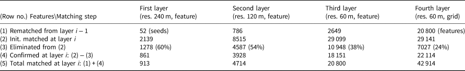
In the study area, 77 historical images (Fig. 1) are used to reconstruct the multi-period historical ice velocity field between 1963 and 1987, including ice velocity fields for 1963–75, 1973–87 and 1985–87. The selection of the time spans is constrained by the available images given the spatial coverage. All the ice velocity fields are then combined into an ice velocity map for 1963–87 by calculating the weighted average of the ice velocity. Taking one of the image pairs involved as an example to demonstrate the feature matching and tracking procedure, 52 seed points (row 1 and first layer in Table 2) are manually measured at the first layer of a four-layer network, which has an image resolution that is four times reduced from the original image. These seed points reconstruct the most general velocity structure of the scene. Then, 2139 detected feature points are matched initially (row 2 and first layer in Table 2), among which 1278 feature points are eliminated according to the threshold of correlation coefficients and the magnitude and direction of velocity vectors within a close neighborhood (row 3 and first layer in Table 2). Therefore, 861 newly matched feature points are confirmed. With the manually measured feature points, a total of 913 matched feature points are present on the first layer (row 5 and first layer in Table 2). In the second layer the resolution is increased to two times the original image. The matched feature points from the first layer are tracked and rematched. The remaining 786 feature points are used to construct the matching constraint (row 1 and second layer in Table 2). The remainder of the process is similar to that of the first layer. In the third layer the original image resolution of 60 m is reached and a total of 20 800 feature points is matched and confirmed (row 5 and third layer in Table 2). The final layer (fourth layer) has the same image resolution as the third layer, the original image resolution of 60 m. A grid with a spacing of 500 m is defined. In total, 22 114 gridpoints (row 4 and fourth layer in Table 2) are matched and confirmed under the constraint of the 20 800 matched feature points (row 1 and fourth layer in Table 2). Consequently, 42 914 matched feature and gridpoints (row 5 and fourth layer in Table 2) are used to calculate the displacements and the ice velocity field in the area. From the first layer to the fourth layer, the rate of eliminated feature points is reduced from 60 to 24% (row 3 in Table 2), which indicates that the automatic matching confirmation rate (reliability) is gradually improved.
Table 2. Intermediate and final results of the hierarchical matching procedure for velocity mapping
The detailed information for feature matching and tracking statistics for all image pairs and accuracy is listed in Table 7. To reconstruct the ice velocity fields of all three periods, 1087 seed points were selected manually to build the initial network at the top level. After the hierarchical feature matching process at all levels, 90 033 matched and confirmed feature points were obtained and applied as constraints to control the dense matching process. Finally, a total of 202 301 velocity vectors were reconstructed for the three mapping periods.
The ice flow velocity at each matched location was calculated according to the displacement between the two corresponding points and the time interval. The ice velocity maps of the Fimbul and Jelbart ice shelves during 1963–75, 1973–87 and 1985–87 in the form of color-coded velocity magnitudes of the matched feature points are presented in Figure 10. No interpolation was performed. For mass-balance estimation purposes, the velocity values of the three maps cover the Jutulstraumen Glacier and the Fimbul Ice Shelf and are used to compute the ice discharge of the three periods from the Jutulstraumen Glacier drainage sub-basin. However, there are velocity data gaps in the Jelbart Ice Shelf and near the grounding line of the Schytt Glacier drainage sub-basin. We used a regional velocity map (Cheng and others, Reference Cheng2019) to fill these gaps, which was produced using 76 Landsat images of 1972–89. Specifically, the velocity values of this map, with a temporal coverage of 1972–87 in this sub-basin, are combined with those produced in this study to produce a velocity field of 1963–87 in the Schytt Glacier drainage sub-basin, using a natural neighbor interpolation implemented in the ArcGIS system (Childs, Reference Childs2004). The matched features in this study and the velocity points of the regional map are used to construct a Voronoi network. The velocities at the network nodes within a neighborhood are weighted to calculate the averaged velocities at gridpoints of the new velocity field. Both the neighborhood and weights are defined based on proximities of the gridpoints to the Voronoi network cells. This method has an advantage of handling clustered scatter points (Gold and others, Reference Gold, Remmele and Roos2006). The resulted velocity field (grid spacing 500 m) of the Schytt Glacier drainage sub-basin has a temporal coverage of 1963–87 and is used for mass-balance estimation. For visualization purposes, the same interpolation method is used to combine this regional velocity map (Cheng and others, Reference Cheng2019) with all matched features in this study to produce a velocity map of the extended region of 1963–89 with a grid spacing of 500 m (Fig. 11).
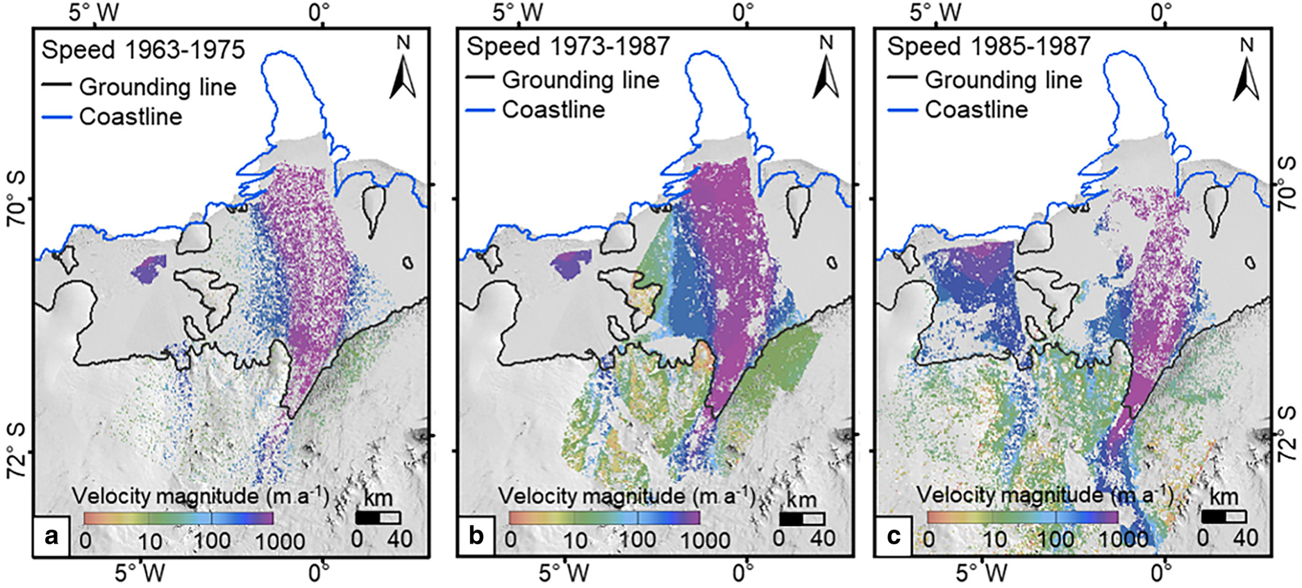
Fig. 10. Ice velocity (magnitude) maps of the region around the Fimbul and Jelbart ice shelves in 1963–75 (a), 1973–87 (b) and 1985–87 (c). The coastline (blue line), including the ice tongue, is extracted from the ARGON mosaic of 1963 (Kim, Reference Kim2004). The grounding line (black line) is from Gardner and others (Reference Gardner2018a). The background image is LIMA image mosaic (Bindschadler and others, Reference Bindschadler2008).
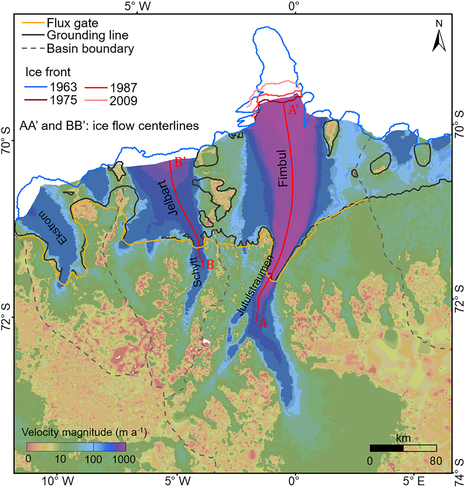
Fig. 11. Ice velocity (magnitude) map of the region around the Fimbul and Jelbart ice shelves from 1963 to 1989. The drainage basin boundaries are from Zwally and others (Reference Zwally H, Mario, Matthew and Jack2012), and the boundary between the Jutulstraumen and Schytt sub-basins is derived based on data from GLIMS (GLIMS and NSIDC, 2005) and REMA (Howat and others, Reference Howat, Porter, Smith, Noh and Morin2019). Four sets of shelf fronts of the Fimbul Ice Shelf are extracted from the ARGON mosaic of 1963 (Kim, Reference Kim2004), MOA mosaic of 2009 (Haran and others, Reference Haran, Bohlander, Scambos, Painter and Fahnestock2014) and Landsat images of 1975 and 1987. The shelf front of the Jelbart Ice Shelf in 1963 is extracted from the ARGON mosaic of 1963 (Kim, Reference Kim2004). The grounding line is from Gardner and others (Reference Gardner2018a). Ice flow center lines AA′ and BB′ are locations of the velocity profiles in Figure 12.
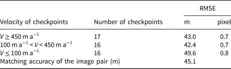
An accuracy assessment of the ice velocity is performed inside the footprint of each individual image pair. Taking an image pair (reference image no. 4 and search image no. 14 in Table 7) that covers the front of the Fimbul Ice Shelf as an example, the ice velocity was derived from two Landsat MSS images, with a time interval of 12 years. We used manually measured checkpoints to estimate the orthorectification errors, which are 42.8 and 44.0 m, respectively. The feature identification error for the Landsat image is 30 m (0.5 pixels). We assessed the matching errors of feature points and gridpoints in separate velocity ranges using manually measured checkpoints, as described in Section 3.3 and Table 8. The average matching error within this image pair is 45.1 m. The ice velocity accuracy of this image pair is calculated according to Eqn (1) as 6.8 m a−1. Finally, the ice velocity values of the individual maps (Fig. 10) and the integrated map (Fig. 11) are estimated by averaging the velocities from the individual image pairs (Table 7) involved in each map. Furthermore, the uncertainties (σ ref, σ src, σ idn and σ mtc) of each map (Table 3) are estimated by applying the error propagation law to the corresponding uncertainties of the involved individual image pairs (Table 7). Equation (1) is then used to estimate the velocity uncertainties (σ vlc) of the produced maps in Table 3. Partly because of the long-time intervals between the image pairs, all maps achieved an accuracy better than 29 m a−1, which is appropriate for analyzing ice flow dynamics and mass changes in the area.
Table 3. Accuracy assessment of the ice velocity maps produced in this study
4.2 Ice velocity changes
We built historical ice velocity maps for three periods before 1987, and compared them with the InSAR ice velocity map for 2007–08 (Mouginot and others, Reference Mouginot, Scheuchl and Rignot2017b). Accordingly, four sets of ice-shelf front boundaries with approximate time tags of the velocity maps are extracted from the Antarctic coastline products or satellite images, including the ARGON mosaic of 1963 (Kim, Reference Kim2004), the MODIS-based MOA 2009 (Haran and others, Reference Haran, Bohlander, Scambos, Painter and Fahnestock2014), and Landsat images from 1975 and 1987. The analysis of the ice velocity changes is primarily facilitated by the velocity comparison along two profiles, namely profile AA′ from along the main trunk of the Jutulstraumen Glacier to the front of the Fimbul Ice Shelf and profile BB′ from along the main trunk of the Schytt Glacier to the front of the Jelbart Ice Shelf (Fig. 12).
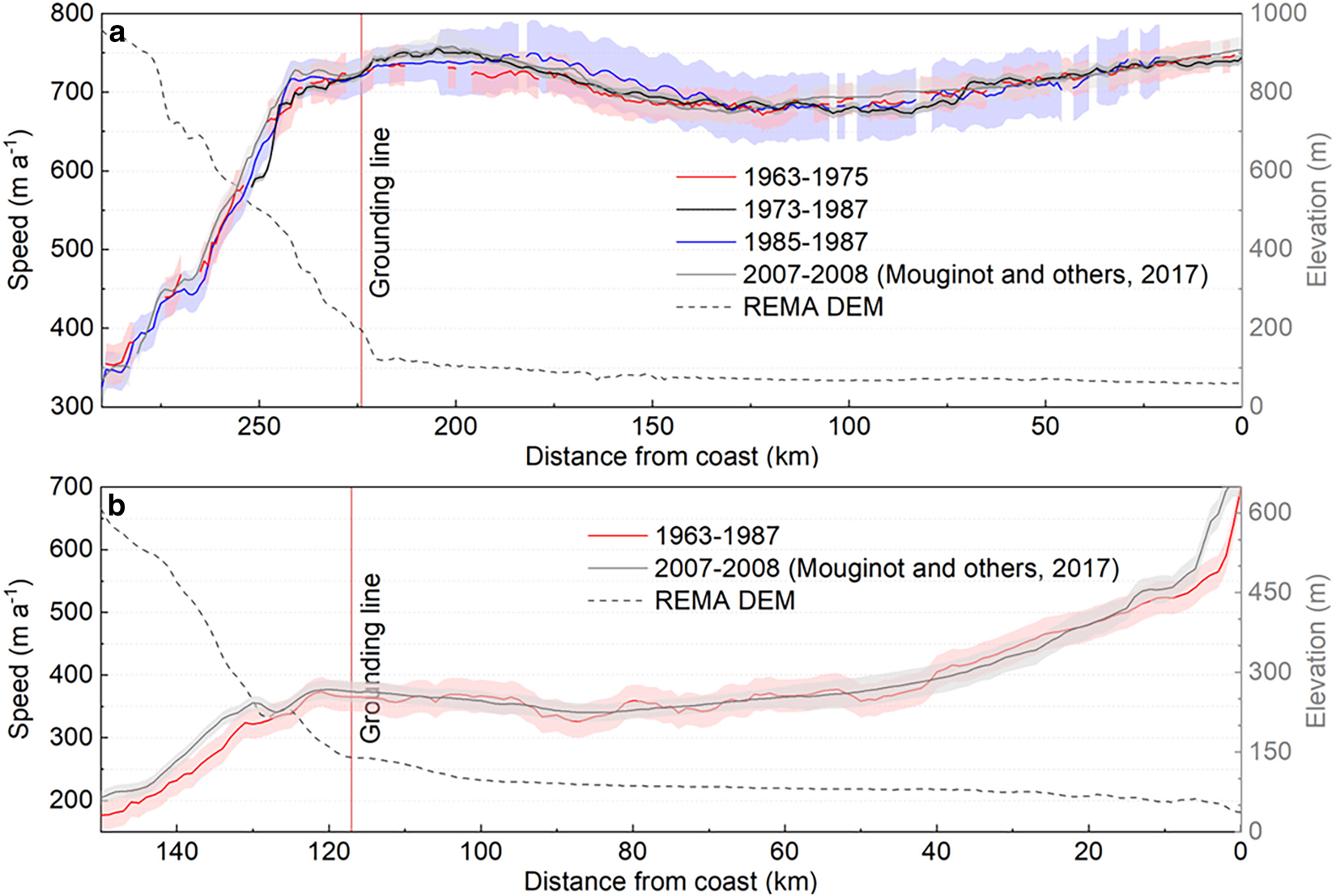
Fig. 12. Ice velocity (magnitude) of four periods from 1963 to 2008 along profile AA′ (a) and that of two periods from 1963 to 2008 along profile BB′ (b). The color bands represent the 1 − σ uncertainties of the corresponding velocities. The profile locations are illustrated in Figure 11. The grounding line is from Gardner and others (Reference Gardner2018a). The velocity uncertainties along the profiles are represented by shadings of the same colors as their velocities.
Along profile AA′, the velocity of the Jutulstraumen Glacier and Fimbul Ice Shelf has an average of 685 ± 22 m a−1 (Fig. 12a). Because of the rapid elevation decrease of ~700 m from the inland interior to the grounding line, the ice flows at an initial velocity of 353 ± 26 m a−1 downstream for ~60 km along the main trunk of the Jutulstraumen Glacier (Fig. 11), and the velocity reaches 725 ± 18 m a−1 at the grounding line. Beyond this point, the glacier feeds the ice shelf at a lower velocity of 680 ± 23 m a−1 in the middle of the shelf. It then increases to 744 ± 7 m a−1 at the ice-shelf front. The confidence intervals of the velocities along AA′ from the four velocity maps from 1963 to 2008 overlap each other, indicating no significant velocity changes over the 45 years. In contrast, the ice flow velocity along profile BB′ is generally 310 ± 24 m a−1 slower than that along profile AA′ (Fig. 12b). The maximum velocity is at the Jelbart Ice Shelf front at 698 ± 26 m a−1. Similarly, the ice velocity of the Schytt Glacier and Jelbart Ice Shelf for 1963–87 does not differ from that for 2007–08, with confidence.
4.3 Mass-balance changes
The mass changes of the ice sheet can be estimated based on the difference between the SMB and the ice discharge from the ice sheet to the ocean. Therefore, the produced historical ice velocity maps provide a unique opportunity to estimate the flux from 1963 to 1987 and investigate the mass balance in the study area using additional later velocity maps. The SMB of a drainage basin is the sum of mass changes occurred during a period through all surface processes within the basin boundary, i.e. the total precipitation of snowfall and rain minus the total sublimation of surface snow, drifting-snow erosion and meltwater runoff (Van Wessem and others, Reference Van Wessem2014). The polar version of the RACMO regional atmospheric climate model (RACMO 2.3p2) provides annual SMB data in Antarctica at a resolution of 27 km (Van Wessem and others, Reference Van Wessem2018). The SMB value in a basin was calculated by summing the SMB estimate values from RACMO 2.3p2 at all cells within the basin boundary. Since the SMB model result does not cover the period prior to 1979, we use the averaged SMB of 1979–89 for these map periods that include time before 1979, e.g. 1963–75, 1973–87 and 1963–87. The SMB of other periods was derived directly from the RACMO2.3p2 results. The drainage basin boundaries (Fig. 11) used in this study are from Zwally and others (Reference Zwally H, Mario, Matthew and Jack2012). To calculate changes of the mass fed into the Fimbul and Jelbart ice shelves separately, the boundary between the Jutulstraumen and Schytt sub-basins was derived based on a combination of two datasets, i.e. glacier outlines of global land ice measurements from space (GLIMS) database (GLIMS and NSIDC, 2005) and ridgelines in the area extracted from the REMA DEM by using the ArcGIS toolbox (Esri Inc., 2020).
On the other hand, ice discharge is the ice flux across the grounding line. We adopt the flux computation procedure introduced by Gardner and others (Reference Gardner2018b). The data used include the ice thickness data of Bedmap-2 (Fretwell and others, Reference Fretwell2013) and the flux gate (FG) from Gardner and others (Reference Gardner2018a). We used the FG from Gardner and others (Reference Gardner2018a) in this study (yellow line in Fig. 11), which are generally defined at locations upstream from the grounding line where ice thickness observations are available. We used an FG width of ~280 m. Assuming that there are no vertical gradients in the ice velocity, the ice flux can be estimated by summing the product of the ice velocity, ice thickness and FG width at each flux node (Gardner and others, Reference Gardner2018a). Using the historical ice velocity maps obtained in this study and the existing ice velocity maps, including the RAMP ice velocity map for 1997 and 2000 (Jezek, Reference Jezek2002), the InSAR ice velocity map for 2007–08 (Rignot and others, Reference Rignot, Mouginot and Scheuchl2011a), and the Landsat 8 ice velocity map for 2014–15 (Scambos and others, Reference Scambos, Fahnestock, Moon, Gardner and Klinger2016), we calculate the ice fluxes through the FGs in the Fimbul and Jelbart regions. The change in flux in the area between the FG and the grounding line is estimated using the SMB in this area (Gardner and others, Reference Gardner2018b). Ice discharge is the flux that crosses the grounding line and is estimated from the ice flux at FG with a correction for the mass change between the FG and grounding line. Consequently, the mass balance, net mass gain (or loss), is estimated by subtracting the ice discharge from the SMB (Table 4).
Table 4. Mass balance of the Jutulstraumen and Schytt sub-basins which the Fimbul and Jelbart ice shelves drain ice from (Fig. 11)
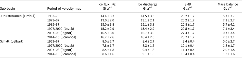
Velocity maps of 1963–87 are from this study and those of 1997–2015 are from Jezek (Reference Jezek2002); Rignot and others (Reference Rignot, Mouginot and Scheuchl2011a); Scambos and others (Reference Scambos, Fahnestock, Moon, Gardner and Klinger2016).
In the Jutulstraumen sub-basin both ice discharge and mass balance maintained a relatively stable level during the study period of 1963–87 (Table 4), resulting in an average mass gain at 6.2 ± 3.6 Gt a−1 during the 24 year period, while the neighboring smaller Schytt sub-basin showed a balanced mass change. Although the three time periods from 1963 to 1987 in Table 4 have 2 year overlaps between them, the mass-balance values are estimated as annual rates (Gt a−1). Therefore, for simplicity of computation, we used the average of the three mass-balance values for the overall mass balance from 1963–87; similarly, assuming the independency between the annual rates, we estimated the uncertainty of the overall mass balance from 1963–87 by applying the error propagation law to the corresponding mass-balance uncertainties of the three periods. This positive mass-balance trend continued in both sub-basins over the subsequent period from 1997 to 2015, as demonstrated by the mass-balance results (Table 4) estimated in this study using the three velocity datasets (Jezek, Reference Jezek2002; Rignot and others, Reference Rignot, Mouginot and Scheuchl2011a; Scambos and others, Reference Scambos, Fahnestock, Moon, Gardner and Klinger2016). The combined results show a long-term positive mass balance of 8.6 ± 3.9 Gt a−1 over 52 years from 1963 to 2015, with 7.3 ± 3.4 Gt a−1 from Jutulstraumen and 1.3 ± 2.0 Gt a−1 from Schytt.
4.4 Discussion
The errors of image orthorectification, feature identification and feature matching, which may be all influenced by the poor quality of the historical images, are the main error sources for ice velocity mapping. However, once two feature points are matched and the motion vector is determined, the accuracy of the estimated velocity improves as the time interval increases. Therefore, we choose images with a longer time span, for example, more than 10 years, to estimate the velocity of the slower motion ice flows in the inland areas and ice rises and those with a relatively short time span, for example, <5 years, to map the fast-flowing glacier and ice-shelf areas. This short time span allows the ice surface features to be tracked before some of them may change due to glaciological processes. According to the velocity comparison results along both the profile of the Jutulstraumen Glacier and Fimbul Ice Shelf and the profile of the Schytt Glacier and Jelbart Ice Shelf (Fig. 12), there were no significant ice velocity changes between 1963 and 2008. In 1967, a major calving separated the ice tongue from the Fimbul Ice Shelf (Wilson, Reference Wilson1977), which caused an area loss of ~5000 km2 (Humbert and Steinhage, Reference Humbert and Steinhage2011) and a front retreat of ~100 km. Since then, the ice tongue had grown back over ~25 km by 2009 (Fig. 11). The time span of the velocity map of 1963–75 covers this ice tongue collapse event in 1967, but the images used are 4 years prior to and 8 years after the event. Thus, the effect of the event on ice flow dynamics is not observed because the resulted signals of velocity changes may be smoothed out by the average velocity of the 12 year time span.
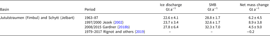
To compare our mass-balance results to other published studies, e.g. Gardner and others (Reference Gardner2018a, Reference Gardner2018b) and Rignot and others (Reference Rignot2019), we combined the mass balance of the two sub-basins in Table 4 and averaged them over the period of 1963–87 (Table 5). The result of 1997/2000 (Jezek) is also a combined rate from Table 4. The row of 2008/2015 Gardner (Reference Gardner2018b) is derived from the result of basin 5 in Gardner and others (Reference Gardner2018b) using an areal ratio between our study area and the basin. Finally, the row of 1979–2017 Rignot and others (Reference Rignot2019) is calculated based on the glacier-scale mass-balance data provided in Rignot and others (Reference Rignot2019). As shown in Table 5, based on the first three studies from 1963 to 2015 the ice discharge in the study area maintained a consistent level at an average rate of ~24.7 Gt a−1. However, it was compensated by SMB over the years at an average rate of ~31.2 Gt a−1, resulting in a positive average mass balance of 6.5 ± 6.2 Gt a−1 for 52 years (1963–2015). Although the areal weighted mass-balance estimate from Gardner and others (Reference Gardner2018b) is used here, this result is in line with our mass-balance estimate of 8.6 ± 3.9 Gt a−1 (1963–2015) for the region. On the other hand, Rignot and others (Reference Rignot2019) presented an approximately balanced mass change in the area during the long period from 1979 to 2017. It should be noted that the velocity field in this study area for 10 years from 1979 to 1989 is not fully mapped in Rignot and others (Reference Rignot2019), but only with very sparsely distributed velocity measurements on the glaciers (Supplementary information of Rignot and others, Reference Rignot2019). The ice discharge was estimated based on these measurements and the later period discharge through a scaling method (Rignot and others, Reference Rignot2019). This study area is one of the major positive mass contributors in Antarctica. Our results revealed a past state of 24 year positive mass balance (1963–87) in the Fimbul and Jelbart regions, which is extended to a 54 year long record of positive mass balance (1963–2017) in the region, when combined with the results of recent studies. This concords with the low positive mass balance of 5 ± 46 Gt a−1, a reconciled estimate from 1992 to 2017 for the entire East Antarctic ice sheet (IMBIE, 2018). Compared to the dramatically retreating and thinning ice shelves in western Antarctica and the collapsed shelves along the Antarctic Peninsula (Rack and Rott, Reference Rack and Rott2004; Rignot and others, Reference Rignot, Velicogna, Den Broeke, Monaghan and Lenaerts2011b; Hogg and Gudmundsson, Reference Hogg and Gudmundsson2017), the Fimbul and Jelbart ice shelves have been stable since the 1960s.
Table 5. Mass balance of the combined basins of the Jutulstraumen and Schytt glaciers which feed the Fimbul and Jelbart ice shelves, respectively
5. Conclusions
This study establishes a framework for the reconstruction of historical ice velocity fields with an implementation in the Fimbul and Jelbart ice shelves area in East Antarctica from 1963 to 1987. The developed methods are essential for investigating the ice sheet response to global climate change in earlier years. A hierarchical network densification approach is developed to meet the challenges of (1) the low quality of historical images from the ARGON and Landsat MSS and TM missions, (2) difficult image orthorectification with limited geometric control data and (3) velocity mapping with altered or untrackable ice features due to glaciological surface processes over long periods. The resulting historical ice velocity maps achieved an overall accuracy better than 29 m a−1 and revealed the ice flow dynamics for 1963–87 in the study area of the Fimbul and Jelbart ice shelves. Combined with existing velocity products, these historical ice velocity maps fill the time gap before 1990 and build a long record of ice velocity maps from 1963 to 2015. This extended historical velocity record reveals that the ice flow velocities of both the Jutulstraumen Glacier and Fimbul Ice Shelf region and the Schytt Glacier and Jelbart Ice Shelf region are relatively stable. The effect of the ice tongue collapse from the Fimbul Ice Shelf in 1967 on the ice velocity pattern is not reflected in the derived maps of average ice velocity due to long time spans. The estimated mass balance of the combined basins of the Jutulstraumen and Schytt glaciers which feed the Fimbul and Jelbart ice shelves, respectively, shows a change rate of 8.6 ± 3.9 Gt a−1 over the 1963–2015 period. Our results indicate that the region's positive mass balance, as estimated in recently published studies, has been maintained since the 1960s. The relatively stable trend in the study area appears to concord with the very low level of positive mass balance of the entire East Antarctic ice sheet. The methodology developed here can be extended to map the historical ice velocity fields of other ice sheets and glaciers.
Acknowledgements
Constructive comments from the editors and two reviewers are greatly appreciated. This work was supported by the National Key Research and Development Program of China (No. 2017YFA0603100), the National Science Foundation of China (Nos. 41730102, 41801335, 41771471, 41941006) and the Fundamental Research Funds for the Central Universities. The authors thank Kee-Tae Kim for the provision of the ARGON mosaic and coastline products of Antarctica (https://etd.ohiolink.edu/apexprod/rws_etd/send_file/send?accession=osu1072898409&disposition=inline), and also acknowledge the United States Geological Survey (USGS) for Landsat images (https://earthexplore.usgs.gov/) and LIMA (https://lima.usgs.gov/), and the National Snow and Ice Data Center for RAMP DEM version 2 (https://doi.org/10.5067/8JKNEW6BFRVD). The authors also thank Mr Tengfei Gao and Mr Yong Huang for their contribution to the data processing and Professor Tong Hao for scientific discussion.
Author contributions
R. L. developed the concept and methodology, and supervised research. T. F. and G. Q. contributed to methodology development and data analysis. Y. L., X. Y. and Y. C. processed data and produced velocity maps. K. W. and S. L. estimated mass balance. All authors wrote, reviewed and edited the final manuscript.
Appendix A
Table 6. Detailed information for the historical remote-sensing images used in Figure 10 (Nos. 1–14) and the inland interior region in Figure 11 (Nos. 15–77)
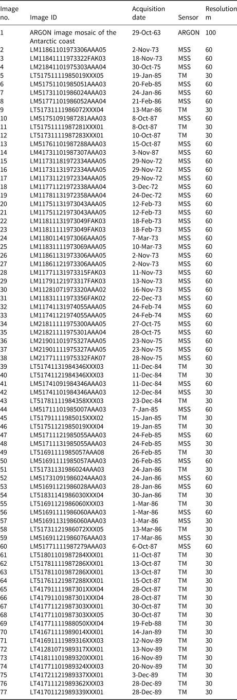
Table 7. Statistical information of seed points used, matched feature and gridpoints, time span, estimated error sources and velocity accuracy for all image pairs that were used for production of the maps from 1963 to 1987
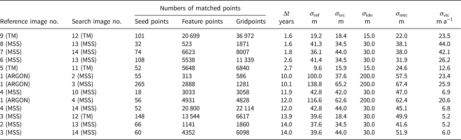
Table 8. Matching accuracy estimated using checkpoints with different ice flow velocities for an image pair


 Open access