


Introduction
Carbon dioxide (CO2) is the most important greenhouse gas directly impacted by human activities. Ancient air preserved in polar ice cores provides extremely important information about the functioning of the carbon cycle in the past (e.g. Reference Etheridge, Steele, Langenfelds, Francey, Barnola and MorganEtheridge and others, 1996; Reference Fischer, Wahlen, Smith, Mastroianni and DeckFischer and others, 1999; Reference PetitPetit and others, 1999; Reference Kawamura, Nakazawa, Aoki, Sugawara, Fujii and WatanabeKawamura and others, 2003; Reference AhnAhn and others, 2004; EPICA Community Members, 2004; Reference Siegenthaler, Stocker, Monnin, Lüthi, Stauffer and SchwanderSiegenthaler and others, 2005). The reconstructed records extend direct measurements of atmospheric CO2 concentrations, which started in 1958 (Reference KeelingKeeling, 1960), and may help us predict future climate under rapidly increasing CO2 more accurately.
The integrity of an ice core as a reliable archive depends on the incorporation followed by the preservation of the original atmospheric signal. It is well known that atmospheric records are smoothed, due to diffusion in the firn column and gradual air trapping in the bubble close-off zone (e.g. Reference Schwander, Stauffer and SiggSchwander and others, 1988; Reference Trudinger, Etheridge, Rayner, Enting, Stur-rock and LangenfeldsTrudinger and others, 2002; Reference Spahni, Schwander, Flückiger, Stauffer, Chappellaz and RaynaudSpahni and others, 2003). However, CO2 diffusion in ice after the air is trapped in bubbles is poorly understood, because the diffusion coefficient is too small to be precisely measured in the laboratory (Reference HondohHondoh, 1996). This uncertainty also limits our understanding of rapid CO2 changes in the atmosphere.
The permeation coefficient (solubility × diffusion coefficient) quantifies gas diffusion in solids. Recent results from a molecular dynamics simulation (Reference Ikeda-Fukazawa, Kawamura and HondohIkeda-Fukazawa and others, 2004) show that CO2 molecules can diffuse orders of magnitude faster in ice than indicated by previous estimates that were based on an interstitial mechanism (Reference Ikeda, Salamatin, Lipenkov, Hondoh and HondohIkeda and others, 2000). The fast diffusion may be due to a new mechanism called the breaking-bond mechanism, where hydrogen bonds break and CO2 hops between stable sites in ice crystals (Reference Ikeda-Fukazawa, Kawamura and HondohIkeda-Fukazawa and others, 2004). However, to date, no good observational estimate of CO2 diffusion in polar ice cores has been reported.
In this study we take advantage of natural CO2 spikes in an ice core associated with refrozen melt layers (hereafter melt layers) to study diffusion that occurred in the ice matrix over thousands of years. We use the gradual decrease of CO2 concentration away from the melt layers, combined with high-resolution analyses of Ca2+ ion, ECM (electrical conductivity measurements), Xe/Ar and Kr/Ar of trapped air to quantify CO2 diffusion in ice. We provide an estimate of the CO2 permeation coefficient in the ice, and discuss the implications of the results for the preservation of CO2 signals in ice cores.
Materials and Methods
The Siple Dome (Antarctica) ice core was drilled between 1997 and 1999. The site is at 81.66° S, 148.82° W, with a present-day annual mean temperature of −25.4°C (Reference Severinghaus, Grachev and BattleSeveringhaus and others, 2001) and accumulation rate of 12.4 g cm−2 a−1 w.e. The total depth of the core is 1003.8 m. While summer air temperatures were generally well below the melting point (Reference Das and AlleyDas and Alley, 2005), surface melting could occur during brief summer warm periods. This happened zero to two times per century during the Holocene (Reference Das and AlleyDas and Alley, 2008).
CO2 measurements were made at the Scripps Institution of Oceanography (SIO) on ice containing bubbles that also included some of the visually distinctive melt layers in the Siple Dome A core (Fig. 1). In each 1 cm depth interval ice samples of 4–6 g were used, and the outer 0.5 cm of the samples was removed with a bandsaw to reduce the possibility of contamination from present atmospheric CO2. The gas extraction and infrared (IR) spectroscopic methods used were described by Reference AhnAhn and others (2004), and are similar to previous methods (Reference Wahlen, Allen, Deck and HerchenroderWahlen and others, 1991; Reference Smith, Wahlen, Mastroianni and TaylorSmith and others, 1997a, Reference Smith, Wahlen, Mastroianni, Taylor and Mayewskib; Reference Fischer, Wahlen, Smith, Mastroianni and DeckFischer and others, 1999). Trapped air was extracted from the ice by mechanical crushing in a double-walled crusher cooled to about −40°C using flowing cold ethanol. The liberated air was collected in small cold traps chilled by closed-cycle helium refrigerators to a temperature of ∼32 K. Trapped air samples were liberated by heating the traps to −60°C and then transferred to an IR absorption cell held at constant pressure and temperature. IR absorption measurements were made several times on each gas sample with a tunable diode laser. The single-mode IR laser output was scanned across a single vibrational–rotational molecular absorption line of CO2 at Doppler resolution. To calibrate the instrument, measurements were made with three air standards of precisely known CO2 concentrations of 163, 240 and 330 ppm. (±0.01 ppm.; personal communication from Carbon Dioxide Group at SIO, 2004) . The standards were introduced over three of the crushed ice samples. This calibration procedure was performed each day. The internal precision was ∼2 ppm. in the concentration range 163–330 ppm.

Fig. 1. Photographs of air bubbles in the Siple Dome ice core: (a) microphotographs of air bubbles around melt layers that were visually defined by small bubbles and relatively transparent layers as shown in (b).
Noble-gas ratios (δ132Xe/36Ar, δ84Kr/36Ar and δ40Ar/36Ar) were analyzed in order to quantify the amount of refrozen melt. These permit us to estimate how much CO2 originated from the meltwater. The gas extraction and measurement on a dual viscous-inlet Finnigan MAT 252 mass spectrometer at SIO have been described previously (Reference Severinghaus, Grachev, Luz and CaillonSeveringhaus and others, 2003; Reference Severinghaus and BattleSeveringhaus and Battle, 2006; Reference Headly and SeveringhausHeadly and Severinghaus, 2007). The depth resolution (4–6 cm) for the noble gases was poorer than the CO2 resolution (1 cm) because a larger ice sample was required for the noble-gas measurements. Around 40–60 g of ice and two stir bars were put in chilled glass vessels, which were attached to a vacuum line. The ambient air was evacuated from the vessel and line for 40 min, after which we closed the valve to stop pumping, and the ice was allowed to melt. The air released from the air bubbles was cryogenically (liquid He) concentrated at 10 K into a stainless-steel dip tube. After warming to room temperature, the gas sample was exposed to a Zr/Al getter at 900°C for 10 min to destroy all the reactive gases, followed by 2 min at 300°C to remove H2. After the gettering process, the remaining noble gases were transferred into a sample tube at 10 K. Finally, ultra-high purity N2 equal to ten times the noble-gas pressure in the vacuum line was added to the sample to add bulk suitable for mass spectrometry. Samples were run against aliquots of a standard gas mixture of commercially obtained N2, Ar, Kr and Xe. δ132Xe/36Ar, δ84Kr/36Ar and δ40Ar/36Ar were normalized using clean marine air outside the laboratory. The pooled standard errors of the triplicate measurements for the Greenland Ice Sheet Project 2 (GISP2) ice core of the Holocene were 3.77‰ and 1.56‰ for δ132Xe/36Ar and δ84Kr/36Ar, respectively, for the measurement conditions.
For Ca2+ ion concentration measurements, we used ∼5 g of ice from the same depths used for CO2 concentration measurements. Ice was prepared at SIO and measured at the Climate Change Institute, University of Maine, using Dionex-500 ion chromatography, where calcium was measured on a CS12A cation-exchange column with 25 mM methanesulfonic acid eluent, a self-regenerating suppressor and a conductivity detector. Sample size was 500 μL.
Results
Excess CO2 associated with melt layers
The annual mean temperature at Siple Dome is −25.4°C (Reference Severinghaus, Grachev and BattleSeveringhaus and others, 2001). However, the site has experienced occasional melting during austral summers (0–2 melt events per century during the Holocene) (Reference Das and AlleyDas and Alley, 2008). The meltwater formed on the snowpack surface percolates into the firn and refreezes at some depth, but rarely percolates >0.2 m, as shown in Figure 2. The snow layer where the melt refreezes is in the form of a fine-crystal size crust that was formed during the previous winter, and has a strong capillary force (Reference Das and AlleyDas and Alley, 2005). Melt layers preserved in the Siple Dome ice core are easily identified visually (Fig. 1) due to lower gas content and reduced bubble size, compared to normal bubbly ice.
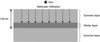
Fig. 2. Schematic diagram for the formation of a refrozen melt layer in the Siple Dome ice cores based on Reference Das and AlleyDas and Alley (2005). Snow melts occasionally in summer under strong insolation. The melt infiltrates (dashed arrow) the summer snow layer (light gray area) and stops and refreezes in the winter layer (dark gray area) by a strong capillary force due to the small size of snow grains.
A 30 cm long ice sample from a depth of 286.7–287.0 m was intensively studied (Fig. 1). The age of the ice is ∼3.04 kyr BP (thousand years before AD1950), and the gas age is ∼2.74 kyr BP (Reference TaylorTaylor and others, 2004; Reference BrookBrook and others, 2005). Annual ice layers are ∼5–9 cm thick at this depth (Reference TaylorTaylor and others, 2004). This section of ice core contains two melt layers (∼1 cm thick), identified by smaller bubble sizes than in the surrounding ice (Fig. 1). The upper (left) melt layer, M1, is thicker than the lower (right) melt layer, M2 (Fig. 1). Distinct dark patches (due to less light scattering in Fig. 1) between M1 and M2 have small bubbles as seen in M1 and M2, suggesting other melt features that do not continue horizontally.
Due to the high solubility of CO2 in liquid water (Table 1), we expect CO2 concentrations in the melt layer to be higher than those in normal bubble ice (Reference Stauffer, Neftel, Oeschger, Schwander, Langway, Oeschger and DansgaardStauffer and others, 1985). Assuming an atmospheric CO2 concentration of 278 ppm (μatm/atm) (Reference IndermühleIndermühle and others, 1999) at the gas age of 2.74 kyr BP and surface pressure at Siple Dome of 937 hPa, we expect 16 230 ppm CO2 (μmol CO2/mol total air) dissolved in 0°C meltwater in equilibrium, 58 times greater than in the atmosphere (Table 1). If a thin film of snowmelt attains solubility equilibrium with the atmospheric air at the surface, and then refreezes rapidly at some greater depth, the excess CO2 in the meltwater can be trapped and preserved in small bubbles in the melt layer. These bubbles can be preserved through the firn metamorphism process and incorporated in mature ice. The CO2 concentration gradient between the melt layer and the neighboring ‘normal’ bubble ice may then cause diffusion through the ice. Excess CO2 (CO2 concentration observed in ice minus atmospheric CO2 concentration) would not be preserved in the melt layer if degassing had occurred fully before the meltwater refroze. Preservation of bubbles in melt layers suggests that refreezing is not slow enough for effective degassing.
Table 1. Solubilities and diffusion coefficients of air components in fresh water for Siple Dome

Our high-resolution (depth interval of 1 cm) study shows that the CO2 concentration in bubbles gradually decreases from 750 to 285 ppm away from M1. Another, smaller, peak is also found around M2 (Fig. 3). CO2 records from colder Antarctic ice-core sites indicate atmospheric concentrations of 278 ppm for the age of our samples (Reference IndermühleIndermühle and others, 1999). The CO2 concentrations in the Siple Dome samples are therefore greater by up to 470 ppm (excess CO2), and clearly do not represent atmospheric values.

Fig. 3. Variation of ECM (proxy for H+) in units of μS (microsiemens), Ca2+ ion, Xe/Ar and Kr/Ar (melt-layer indicators) and CO2 around the melt layers shown in Figure 1. The δ(Xe/Ar) and δ(Kr/Ar) values are normalized to present atmospheric air. The minor and rather constant enrichment of Kr and Xe are due to gravitational settling in the firn and do not indicate substantial melting/refreezing. Finely hatched vertical bars indicate melt layers. The thicknesses and positions of the melt layers vary between the two bars around each melt layer.
The existence of refrozen meltwater in M1 and M2 is supported by our analyses of 132Xe/36Ar and 84Kr/36Ar as shown in Figure 3. Xe/Ar and Kr/Ar in glacial ice are useful indicators of extensive snowmelting and refreezing, as Xe and Kr are about four and two times as soluble in liquid water as Ar, respectively (Reference Severinghaus, Grachev, Luz and CaillonSeveringhaus and others, 2003). Our data show significantly enriched Xe/Ar and Kr/Ar for ice that includes the visible melt layers, M1 and M2, relative to normal layers, indicating the existence of the refrozen meltwater in M1 and M2.
In order to quantitatively determine the excess CO2 resulting from the refrozen melt, we use the melt-sensitive isotope ratios, 132Xe/36Ar and 84Kr/36Ar. Considering the solubility of the noble gases at 0°C, the gravitational fractionation in the firn layer and the Ar loss from the bubbles during sample handling or bubble close-off, our calculation using the Xe/Ar and Kr/Ar data gives the volume ratio of liquid water to pore air (see Appendix B for details). This is accomplished by solving three equations for three unknowns with three observed quantities: Xe/Ar, Kr/Ar and 40Ar/36Ar.
For the ice sample that includes normal layer, M1 and the partial-melt layer between M1 and M2, a volume ratio of liquid water to pore air of 1.38 is obtained. Using the total air in the sample (4.7 ± 0.5 cm3 STP (standard temperature and pressure)), we calculate that the volume of refrozen melt is 6.5 ± 0.7 cm3. The total air content of the ice samples was calculated with (1) the volumes of ice from the normal and melt layers, (2) bubble-volume ratios (air-content ratios) of normal melt layers and (3) the air content of the normal layers, which was estimated from the average over the Holocene as the air content is almost constant in that period (Reference Severinghaus and BattleSeveringhaus and Battle, 2006). The estimated volume of refrozen melt is comparable to our visual observation. The volume of visual melt layer (defined by ice with smaller bubbles than in the normal layer) is 16.4 ± 1.4 cm3 (13.9 ± 0.7 cm3 from M1; 2.5 ± 0.7 cm3 from the partial-melt patch between M1 and M2). This visual refrozen ice volume is apparently bigger than our estimation of the volume of refrozen melt because the volume of the visual melt layer includes pre-existing ice (firn), where meltwater filled the void space and refroze. The difference between estimates based on Xe/Ar, Kr/Ar, 40Ar/36Ar and the visual observation is 40 ± 8%, close to the porosity of snow at the surface, 56% (ice density at the surface = 0.4 g cm−3; personal communication from J. Fitzpatrick, 2007), indicating that Xe, Kr and Ar were close to equilibrium with the ancient atmosphere and were trapped in melt layers. Therefore, we can also expect that the melt at the surface was in equilibrium with ancient atmospheric CO2 which was trapped in M1.
For additional confirmation for our diffusion model, we estimate the total CO2 trapped in M1 at the snow surface with the calculated volume of purely refrozen melt in M1 from Xe/Ar and Kr/Ar measurements:

This agrees with the integration of the observed excess CO2 in the upper part of M1 (including the upper half of M1) of ∼5.4 × 10⁻⁹ mol cm−2. This agreement supports the assertion that the CO2 profile around the melt layers was formed by diffusion from the melt layer. The accuracy of the above estimate is possibly limited by different degrees of equilibration of different gases in the meltwater. For example, Xe should approach equilibrium more slowly than CO2, due to its lower diffusivity but within the same order (Table 1). In this estimate we assume gas diffusion in ice does not change the profile of Xe/Ar and Kr/Ar.
CO2 diffusion in the ice
The gradual decrease in CO2 away from the melt layers is consistent with CO2 diffusion over the past 2.74 kyr, and agrees reasonably well with predictions from a molecular volume-diffusion model (Fig. 4) (Reference Neftel, Oeschger, Schwander and StaufferNeftel and others, 1983; see Appendix A for details). For simple one-dimensional curve fitting, we utilize the CO2 mixing ratio data from the normal and melt layers. The CO2 concentrations from the partial-melt layer between the two melt layers have higher values than those in the fitting curve, due to additional CO2 in the partial-melt patches. Thinning of vertical layers with increasing depth due to the flow of the ice is taken into account. In our numerical approach, we utilize an age–depth profile from CH4 correlation with the Greenland ice core (Reference BrookBrook and others, 2005) and a depth–density profile (personal communication from J. Fitzpatrick, 2007) for the real depth, pressure and porosity parameters in each time-step rather than estimation based on the assumption of constant snow accumulation rate and porosity (Reference Neftel, Oeschger, Schwander and StaufferNeftel and others, 1983). For example, the porosity profile for the numerical modeling was estimated from the density profile for the top 300 m (ϕ = 1 − (ρ bubbly ice/ρ bubble-free ice)) rather than using confining ice pressure, because air pressure in bubbles at shallow depth is not in equilibrium with the confining hydrostatic ice pressure, as shown in the top 300 m of the Vostok (Antarctica) ice core (Reference Lipenkov and HondohLipenkov, 2000). For depths >300 m we obtained porosity from the gas content (∼0.11 cm3 air (STP) g−1 ice) (Reference Severinghaus and BattleSeveringhaus and Battle, 2006) divided by confining pressure in the atmosphere (personal communication from J. Fitzpatrick, 2007) and the density of bubble-free ice (0.917 g cm−3). Two approaches were used for estimating the vertical thinning factor, α (see Appendix A for details): (1) assuming constant strain-rate thickness and (2) utilizing the paleo-accumulation rate estimated from the isotopic temperature proxy (Reference BrookBrook and others, 2005). The latter estimations of α are 89% and 57% of the former for the last 2740 years and ∼18.5–80 kyr, respectively. However, in the 2740 year modeling and curve fitting, using the two different thinning factor approaches gave no difference in the estimated permeation coefficient within the range of uncertainty of curve fitting.

Fig. 4. Comparison of excess CO2 concentration from the observations (circles) to the prediction by modeling (solid curve for M1 and dashed curve for M2). c 0 and c are the CO2 concentrations before and after diffusion, respectively. Different c/c 0 values are used for M1 and M2. The horizontal bars through circles are depth intervals of samples. Gray areas denote melt layers (M1 and M2) with averaged thicknesses and positions. The actual thicknesses vary along the melt layers, as noted in Figure 3. The model curves are fitted to CO2 observations in the melt and normal layer ice, but not to observations between the two melt layers, where partial-melt patches exist.
We assume that the permeation coefficient (diffusion constant × solubility) is almost constant over a wide range of solubility (see Appendix A), and the same value of the permeation constant of CO2 in ice was applied for the two melt layers. The good fit of the model to the data supports our proposition that the CO2 originally trapped in the melt layer has diffused through the ice for thousands of years. The baseline CO2 levels far from the melt layers are still slightly higher than in the Taylor Dome (Antarctica) and Dome C (Antarctica) ice records (Reference IndermühleIndermühle and others, 1999), by 11 ppm on average. The reason for this discrepancy is not clear, but may be due to microscale refreeze of melt (Reference AhnAhn and others, 2004) or differences in laboratory standard scales for CO2.
Alternative explanations for the excess CO2 in the ice adjacent to the distinctive melt layers include: (1) visibly undetected micro-melt layers, (2) carbonate–acid reaction (Reference DelmasDelmas, 1993; Reference Anklin, Barnola, Schwander, Stauffer and RaynaudAnklin and others, 1995, Reference Anklin1997; Reference Barnola, Anklin, Porcheron, Raynaud, Schwander and StaufferBarnola and others, 1995; Reference Smith, Wahlen, Mastroianni and TaylorSmith and others, 1997a, Reference Smith, Wahlen, Mastroianni, Taylor and Mayewskib) and (3) oxidation of organic compounds abiologically (Reference Tschumi and StaufferTschumi and Stauffer, 2000) or biologically (Reference Campen, Sowers and AlleyCampen and others, 2003).
If the excess CO2 of hundreds of ppm around M1 and M2 originated from micro-melt layers, we would observe the same characteristics in the excess Xe/Ar and Kr/Ar as in the excess CO2. However, we do not detect significantly elevated Xe/Ar and Kr/Ar above M1 and below M2, in areas where we do see significant excess CO2 (Fig. 3). These observations strongly support our idea that excess CO2 in the normal layer formed by diffusion from the melt layers. In between M1 and M2, the resolution prevents us from comparing the CO2 with Xe/Ar or Kr/Ar. Different degrees of saturation of the gas species and different degassing during freezing may explain the difference between CO2 and the Xe/Ar and Kr/Ar profiles. However, the diffusion coefficients of these gas species in water are of the same order (Table 1), supporting our diffusion model. It is important to note that we are assuming that diffusion of Xe, Kr and Ar in ice is negligible compared to that of CO2. However, recent work suggests that Ar may diffuse more rapidly in ice than Kr and Xe (Reference Severinghaus and BattleSeveringhaus and Battle, 2006). If Ar is more mobile than Kr and Xe, the Kr/Ar and Xe/Ar ratios will decrease outside the melt layers but increase in the melt layers. To date, the permeation coefficients of Xe, Kr and Ar are unknown. Thus, exact evaluation of this effect remains elusive. However, the good agreement of two noble-gas datasets in all layers other than melt layers would have to be fortuitous if this effect is important. For this reason we consider the scenario unlikely.
The concentration of dissolved Ca2+ can be used to estimate the upper limit of the amount of CaCO3 that potentially could have reacted with H+. There is no significant correlation between the excess CO2 and the dissolved Ca2+ or ECM (a proxy for H+), as shown in Figure 3. Moreover, assuming that all the Ca2+ is produced from the reaction between CaCO3 and H+, the potential excess CO2 is ∼17 ppm on average. Thus, the amount of Ca2+ is too small to explain our observations (excess CO2 of up to 470 ppm); 1 μg Ca2+ per kilogram of ice can explain at most 7 ppm of excess CO2 by the carbonate–acid reaction.
Oxidation of organic compounds has been proposed to be at least as important as acid–carbonate reactions for CO2 production (e.g. 2H2O2 + HCHO → 3H2O + CO2) in some ice cores (Reference Tschumi and StaufferTschumi and Stauffer, 2000). However, H2O2 data for the top 100 m of the Siple Dome ice core show H2O2 concentrations near or below the detection limit of ∼0.02 μm, except at 0–2.5 m depth (Reference McConnellMcConnell, 1997). H2O2 is one of the major oxidants in snow. These H2O2 concentrations at Siple Dome are much lower than those found in other Antarctic ice cores (Reference McConnellMcConnell, 1997). The data for other important oxidants such as CH3COO− and HCOO− (Reference Tschumi and StaufferTschumi and Stauffer, 2000) are not available. However, the excess CO2 due to this process may be less than in Greenland ice cores, where the dust and oxidant contents are greater than in Antarctic ice cores by an order of magnitude and several times, respectively (Reference Tschumi and StaufferTschumi and Stauffer, 2000), and the excess CO2 is ∼30 ppm for the Holocene (Reference Anklin, Barnola, Schwander, Stauffer and RaynaudAnklin and others, 1995; Reference Barnola, Anklin, Porcheron, Raynaud, Schwander and StaufferBarnola and others, 1995). Thus, oxidation of organic compounds cannot explain the high excess CO2 of up to 470 ppm.
We conclude that the three alternative mechanisms cannot explain the excess CO2 distribution around the melt layers, and that the concentration profile is most likely to have formed by the diffusion of CO2 through the ice matrix from the refrozen melt (M1, M2 and partial-melt) layers. However, we cannot exclude the possibility of invisible micro-melt layers due to our unproved assumption that diffusion did not change Xe/Ar and Kr/Ar profiles. In this case, our estimation of the permeation coefficient of CO2 in the following part of this section would be a maximum and provide an upper limit on the impact on CO2 mobility of the ice-core records.
From the best-fit calculation, the permeation coefficient of CO2 (the product of the diffusion constant and the solubility) in ice is ∼4 × 10⁻²¹ m−1 s−1 mol Pa−1 at −23°C (time-averaged temperature) as seen in Figure 4. We find higher CO2 concentrations in the samples that include partial-melt layers than in the modeling because the former have lower gas content than the normal bubble ice. Our result for the permeation coefficient of CO2 is independent of the Xe/Ar and Kr/Ar data. We estimate that the amplitudes of the CO2 variation in the measured core segment are ∼30% and ∼20% of the initial amplitude, c 0, for M1 and M2, respectively (Fig. 5). The different ratios are due to the different melt-layer thicknesses.

Fig. 5. Modeling of the smoothing of a 10 year spike (thick solid line) of the atmospheric CO2 record by diffusion in the deep Siple Dome ice sheet. Distance from the center of the spike is converted to the timescale. Smoothing by gas-age distribution (thick dash–dot curve) is estimated assuming a Gaussian distribution (σ = 12.74 years; full width at half height = 30 years). Two sets of thinning factors are used: α1, assuming constant strain rate with depth, and α2, utilizing snow accumulation rates and annual-layer thicknesses (see Appendix A for details). c 0 and c are the CO2 concentrations before and after diffusion, respectively.
Our result for the CO2 permeation coefficient is an order of magnitude greater than that estimated from the Dye 3 (Antarctica) ice core (1.3 × 10⁻²² m−1 s−1 mol Pa−1 at −20°C) (Reference Neftel, Oeschger, Schwander and StaufferNeftel and others, 1983). This discrepancy is probably due to the inaccurate assumption that the Dye 3 ice core has never changed to clathrate ice from bubbly ice (Reference Neftel, Oeschger, Schwander and StaufferNeftel and others, 1983). The Dye 3 ice-core segment studied for diffusion was selected from the bottom of the bubble-ice–clathrate transition zone (depth = 1616 m; 31.1 kyr), where gas species go into the ice lattice and bubbles shrink and finally disappear (Reference Neftel, Oeschger, Schwander and StaufferNeftel and others, 1983). The formation of clathrate begins at a depth of 1200 m (14.7 kyr) (Reference Neftel, Oeschger, Schwander and StaufferNeftel and others, 1983) and possibly significantly changes the diffusion of CO2. Reference Salamatin, Hondoh, Uchida and LipenkovSalamatin and others (1998) deduced that the diffusion coefficient of air in hydrate crystals is at least two orders of magnitude less than the diffusion coefficient of air in the ice matrix. Thus, CO2 may be bound more in clathrate crystals than in ice. In addition, the solution of gas in clathrate crystals into the ice matrix is much less dependent on hydrostatic pressure than in bubbles, following Equation (A3).
Dividing the permeation coefficient by the solubility gives the diffusion coefficient. Unfortunately, the solubility of CO2 in ice is not well known at present, as it is too small to be measured precisely (Reference HondohHondoh, 1996). We calculate the CO2 diffusion coefficient in the ice matrix at −23°C to be >1.3 × 10⁻¹³ m2 s−1 for a solubility of CO2 in ice <4.5 × 10⁻⁸ mol m−3 Pa−1 (Reference Neftel, Oeschger, Schwander and StaufferNeftel and others, 1983). Improved measurement of CO2 solubility in ice in the future would allow a better estimate of the diffusion coefficient of CO2 in polar ice. We estimate the solubility of CO2 in ice to be 5.1 × 10⁻¹¹ mol m−3 Pa−1 at −23°C, using the permeation coefficient divided by the modeled diffusion coefficient of 7.8 × 10⁻¹¹ m2 s−1 (Reference Ikeda-Fukazawa, Kawamura and HondohIkeda-Fukazawa, 2004, table 3).
Smoothing of the CO2 record in polar ice
Significant diffusion for thousands of years in the ice sheet might smooth rapid atmospheric changes and this would be extremely important in interpreting ice-core records. Well-known smoothing processes include gas diffusion in the firn layer and gradual bubble close-off at the transition from firn to ice, the effect of which can be roughly approximated by a Gaussian filter corresponding to the gas-age distribution (e.g. Reference Schwander, Stauffer and SiggSchwander and others, 1988; Reference Trudinger, Etheridge, Rayner, Enting, Stur-rock and LangenfeldsTrudinger and others, 2002; Reference Spahni, Schwander, Flückiger, Stauffer, Chappellaz and RaynaudSpahni and others, 2003).
Based on our observations and modeling, the smoothing of the CO2 concentration by diffusion in deep ice is of the order of a few centimeters in our samples and, thus, negligible compared to the smoothing by the gas-age distribution at that depth (∼30 years, corresponding to diffusion in the depth interval of ∼100 cm). However, at greater depths the smoothing by CO2 diffusing through the ice matrix may become larger.
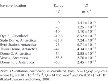
A 10 year instantaneous atmospheric CO2 spike (corresponding to 1.55 m at the bubble close-off depth) is modeled with the permeation coefficient obtained in the shallow Siple Dome ice. The diffusion coefficient may significantly increase with greater depth due to geothermal warming. Results from the molecular simulation suggest that the diffusion coefficient approximately doubles for each 20°C increase in temperature (Reference Ikeda-Fukazawa, Kawamura and HondohIkeda-Fukazawa and others, 2004) as shown in Table 2. At a depth of 960 m (∼80 kyr) at a location near the Siple Dome core site, the ice temperature reaches −4°C (269 K) (Reference EngelhardtEngelhardt, 2004), 19°C higher than at the shallow depth where we estimated the CO2 permeation coefficient. Combining the depth–temperature profile with the temperature dependence of the diffusion coefficient (Reference Ikeda-Fukazawa, Kawamura and HondohIkeda-Fukazawa and others, 2004), we calculated permeation coefficients for modeled depths. Solubility of CO2 in ice was assumed constant because the solubility/temperature relation is unknown.
Table 2. Temperature dependence of CO2 diffusion coefficient in ice
The results from the 80 kyr simulations for two different estimations of thinning factor suggest that diffusion in deep ice may smooth the CO2 concentration profile on decadal timescales, and at the age of ∼60–70 kyr (Siple Dome depths of ∼930–950 m) may be comparable to smoothing by diffusion in firn (Fig. 5). There are no decadal CO2 data for ice that is 80 kyr old. However, the CO2 record from the Siple Dome ice core shows significant variation of CO2 on millennial timescales for the past 40 kyr (Reference AhnAhn and others, 2004). Ice cores from colder sites than Siple Dome would experience slower CO2 diffusion in deep ice. The formation of clathrate ice (bubble-free ice) at depths from 500 to 1200 m (∼25–65 kyr) at other Antarctic cold-drilling sites (Vostok, Dome Fuji and EPICA Dome C) is expected to result in highly reduced gas diffusion (Reference Salamatin, Hondoh, Uchida and LipenkovSalamatin and others, 1998).
Discussion and Directions for Future Work
The processes of gas diffusion related to variable physical properties of ice are still not well known. Thus, our volume-diffusion model should be investigated further. As discussed in the previous section, our interpretation of the noble-gas species is limited due to our lack of knowledge of their diffusion properties. Nonetheless, our study provides an important upper limit on the CO2 permeation coefficient in ice cores. The true value of the permeation coefficient could be lower than we estimate if micro-melt layers around the visible melt layers contribute to the excess CO2 in our data.
Processes other than volume diffusion may be important but are difficult to quantify. For example, there is evidence of the existence of melt at triple junctions of grain boundaries in polar ice (Reference Mulvaney, Wolff and OatesMulvaney and others, 1988). Thus, CO2 may dissolve and migrate in the liquid vein, while noble-gas species, with lower solubility, may mostly stay at the original sites. If this is the case, the diffusion via the liquid vein or ice grain boundaries may be governed directly by the grain-growth rate, as suggested from an ion chemistry study (Reference Barnes, Wolff, Mader, Udisti, Castellano and RöthlisbergerBarnes and others, 2003).
Our extension of the modeling results at shallow depth (corresponding to 2.74 kyr BP) to greater depths is limited by uncertainties in basic parameters and requires further study. For example, the assumption of Henry’s law for the CO2 solubility in ice may not be valid through all pressure ranges. The temperature dependence of CO2 solubility in ice is not considered since it is unknown. The dependence of the diffusion coefficient on temperature should be constrained, based on observations. Moreover, better constraints on the porosity–depth profile, which is one of the key parameters in our model, are needed.
In addition, the permeation coefficient of CO2 may vary from core to core and depth to depth due to the variable physical properties of the ice. Studies with ice samples from various physical conditions (e.g. temperature, pressure, crystal growth rate) with different ice cores will better constrain the permeation coefficient.
Our estimation of the CO2 concentrations in the melt layers is based on the experimental results for ice samples that include both the melt and normal layers. We assume constant gas extraction efficiency (gas extracted ÷ gas in ice before extraction) for both the normal and melt layers. If the gas extraction efficiency varies with the size of the bubbles (small bubbles in the melt layers and large ones in the normal layers), our measurements are not precise enough to detect differences in efficiency. Other techniques that allow 100% extraction efficiency such as sublimation of ice (e.g. Reference Güllük, Slemr and StaufferGüllük and others, 1998) or melting of ice (e.g. Reference Kawamura, Nakazawa, Aoki, Sugawara, Fujii and WatanabeKawamura and others, 2003) could improve the estimation.
Our results also imply the possibility of an artifact in δ13C of CO2 records due to different diffusion rates of 12C and 13C. Another possible implication is change of CO2 mixing ratio in ice cores during storage.
Conclusions
Refrozen melt layers in the Siple Dome ice core contain excess CO2 due to the high solubility of CO2 in the meltwater. Our analyses of samples from the Siple Dome ice core show a gradual decrease of CO2 away from two refrozen melt layers. The excess CO2, combined with noble-gas data (Xe/Ar, Kr/Ar) and chemical and electrical properties of the ice, suggest that an initial CO2 spike diffused through the ice. By modeling the CO2 molecular diffusion, we calculate the permeation coefficient (the product of solubility and the diffusion coefficient) of CO2 in ice to be ∼4 × 10⁻²¹ m−1 s−1 mol Pa−1 at −23°C. This rate indicates smoothing of the CO2 record by diffusion is one to two orders of magnitude smaller than the smoothing by diffusion in the firn at the depth of 287 m (gas age = 2.74 kyr BP) in the Siple Dome ice, and so does not degrade the record. However, applying the permeation coefficient to greater depth (equivalent to tens of thousands of years) in the Siple Dome ice core suggests an impact on smoothing of the CO2 records on a decadal scale. Processes other than volume diffusion may be important but are difficult to quantify. Further studies should include the mechanism of the diffusion, dependence of the diffusion coefficient on temperature and solubility of the gas in the ice. Formation of clathrate seems to significantly hinder the CO2 diffusion and will help preserve atmospheric records.
Acknowledgements
We thank S. Sneed at the Climate Change Institute, University of Maine, for the major-ion concentration measurements, and A. Bollenbacher at SIO for the preparation of the CO2 air standards. We also thank S. Das, B. Deck, T. Ikeda-Fukazawa, R. Alley, K. Kawamura and J. Fitzpatrick for invaluable comments. Discussion with J. Severinghaus, B. Stauffer, J. Schwander, S. Kim, J. Schmitt and an anonymous reviewer greatly improved the paper. We are grateful to D. Peel for his attention and handling of the manuscript. Ice cores were cut by J. Rhoades at the US National Ice Core Laboratory. This work was supported by the Office of Polar Programs of the US National Science Foundation (NSF OPP 99-80619) to M.W. and the Gary Comer Science and Education Foundation.
Appendix A Volume-Diffusion Model
Elevated CO2 diffuses from a melt layer to bubbles within a normal layer through the ice matrix. The smoothing of the CO2 concentration is calculated from molecular volume diffusion with constant mixing ratio, c 0, in a certain width of the melt layer (Reference Neftel, Oeschger, Schwander and StaufferNeftel and others, 1983). The CO2 flux by the diffusion is:
where j (mol m−2 s−1) is the flux of CO2 by diffusion, D (m2 s−1) is the diffusion constant of CO2 in ice, c E (mol m−3) is the concentration of CO2 dissolved in the ice and x eff (m) is the effective vertical distance accounting for thinning by ice flow. This is related to the original distance, x, and the thinning factor, α(t):
Equation (A2) is needed to incorporate the effect of thinning on the distance CO2 diffuses in the ice as a layer is buried. Also, we assume that melt layers are horizontally uniform, which is likely to be valid for the short distance (a few centimeters) involved.
The c E is related to the parameter we measure, the CO2 mixing ratio in the bubble air, c B, bubble air pressure, p(Pa), as function of time and depth, p(z(t)), and CO2 solubility in ice, S (mol m−3 Pa−1), according to Henry’s law:
The total CO2 concentration per unit volume of bubble ice, c tot (mol m−3), requires the porosity of the ice, ϕ, and is:
The diffusion equation then becomes:

The middle part of Equation (A5) can be written as:

where we assume S is constant. The second and third terms in square brackets in Equation (A6) are smaller than that in the first square bracket with order of >O(102) and >O(103), respectively. Therefore, we simplify Equation (A6):

As we found ![]() is greater than the other terms in Equation (A7) with order of O(10) for most times and locations in ice for the 2740 year simulation, Equation (A6) can be written as:
is greater than the other terms in Equation (A7) with order of O(10) for most times and locations in ice for the 2740 year simulation, Equation (A6) can be written as:

Also, the righthand side of Equation (A5) becomes:

Thus, Equation (A5) becomes:

For each time-step, we calculate the CO2 mixing ratio in bubble air for each nth position ![]() with a constant distance interval (Δx = 1 mm for the 2740 year simulation; 0.155 m for the 80 kyr simulation). Equation (A10) can be discretized as:
with a constant distance interval (Δx = 1 mm for the 2740 year simulation; 0.155 m for the 80 kyr simulation). Equation (A10) can be discretized as:

In the finite-difference equation, realistic α(t), ϕ and p are estimated for each time-step. The thinning factor, α(t), is determined by two different methods: (1) assuming a constant strain rate with depth, which is
where H is the thickness of the ice sheet and z(t) is depth below the surface, which is estimated from the independent depth–gas age profile (Reference BrookBrook and others, 2005), and (2) utilizing the paleo-accumulation rate estimated from the isotopic temperature proxy (Reference BrookBrook and others, 2005):

A realistic ϕ is estimated from the gas content in ice of ∼0.11 cm3 g−1 STP (Reference Severinghaus and BattleSeveringhaus and Battle, 2006) and accumulated ice load at depths >300 m (personal communication from J. Fitzpatrick, 2007), assuming that the pressure of air in bubbles equilibrates with the confining pressure. At shallow depth (<300 m), this assumption is not valid and ϕ is estimated using ice-density data (personal communication from J. Fitzpatrick, 2007) at time t:
Hydrostatic pressure, p, is estimated from depth–density profiles (personal communication from J. Fitzpatrick, 2007).
For the 80 kyr modeling, we use a diffusion coefficient, D, which varies with temperature (Reference Ikeda-Fukazawa, Kawamura and HondohIkeda-Fukazawa and others, 2004, table 3).
The constant parameters used for the Siple Dome ice studied are:

Appendix B Volume Ratio of Refrozen Liquid Water to Bubble Air
We have modeled the effects of the formation of melt layers on SKr/Ar, SXe/Ar and δ40Ar/36Ar in air bubbles in ice cores. The detailed model will be reported elsewhere. Briefly, we assume that 36Ar, 40Ar, Kr and Xe in air measured in an ice-core sample are affected only by gravitational settling, melt and gas loss as follows (units are moles of gas):

We also assume that all the dissolved gas is retained during the refreezing process. We use this model to invert the δKr/Ar, δXe/Ar and δ40Ar/36Ar measurements for the firn diffusive column depth, z, gas loss during ice-core storage, F, and the volume ratio of refrozen liquid water to bubble air at ambient pressure, γ. We use the equations above, as well as the ideal gas law (pV = nRT) and the barometric equation (p = p 0 exp(mgz/RT)), to derive the following system of equations, which can be solved by iteration for γ, F and z (all variables defined below):


