


Introduction
Molecular modeling is becoming increasingly important in many different areas of fundamental and applied research (Cygan Reference Cygan2001; Lu et al. Reference Lu, Aksimentiev, Shih, Cruz-Chu, Freddolino, Arkhipov and Schulten2006; Medina, Reference Medina2009). This is due not only to the development of high-performance computing in recent decades but also because of increasingly user-friendly molecular modeling software, allowing for high-throughput screening of large classes of molecules. This is especially true for life-science related research, which traditionally has spearheaded the development and design of molecular modeling software and forcefield tools. However, due to the wide use of molecular modeling in different scientific disciplines, custom-made setup or analysis tools specifically tailored to the user’s system are often required. This is because of the need to perform specific tasks that topology tools aimed towards modeling of biomolecules normally do not offer. Examples of this include the ability to perform: (1) automatic atomtype assignment for less common or system-specific forcefields; or (2) the ability to find bonds and angles across the periodic boundary conditions (PBC) for periodic slabs or layered molecules, such as graphene and graphite oxides, zeolites, clay minerals, layered double hydroxides, etc.
In this context and especially for scientists lacking comprehensive programing skills, MATLAB, R, and similar software packages offer an attractive and versatile environment for scientific computing with simple yet robust scripting languages, plotting capabilities, and the possibility to display or copy data variables into spreadsheets. In fact, a handful of MATLAB and R packages for trajectory or statistical analysis focusing on biomolecules has been developed (Dien et al. Reference Dien, Deane and Knapp2014; Dombrowsky et al. Reference Dombrowsky, Jager, Schiller, Mayer, Stammler and Hamacher2018; Kapla & Lindén Reference Kapla and Lindén2018; Matsunaga & Sugita Reference Matsunaga and Sugita2018). This work presents the Atomistic Topology Operations in MATLAB (atom) library – a large collection of >100 modular MATLAB scripts and sub-routines (e.g. functions) under an open source license (simple BSD) which comprise a general framework for construction, manipulation, and analysis of atomistic systems, with the option of incorporating topological and forcefield information. In contrast to the above-mentioned MATLAB and R trajectory packages, the focus here lies not on the modeling of biomolecules but rather on the investigation of especially periodic inorganic structures, such as slabs and layers that have well defined unit cells (UC) stretching over the PBC.
Because the atom function calls can be invoked from the command line as well as from within custom-made MATLAB scripts and programs, the atom library is especially well suited to batch-mode operations. In particular, the atom library may be useful for scientists with an interest in modeling inorganic and geochemical systems. This is because apart from parsing the input or output of basic coordinate files (.pdb|.xyz|.gro|.cif), the atom library can also be used to output basic molecular topology files (.lmp|.itp|.psf) for the CLAYFF forcefield (Cygan et al. Reference Cygan, Liang and Kalinichev2004) and INTERFACE (Heinz et al. Reference Heinz, Koerner, Anderson, Vaia and Farmer2005, Reference Heinz, Lin, Kishore Mishra and Emami2013) for certain geochemical systems/software, which are used in molecular modeling software such as LAMMPS, Gromacs, NAMD and RASPA2 (Plimpton Reference Plimpton1995; Phillips et al. Reference Phillips, Braun, Wang, Gumbart, Tajkhorshid and Villa2005; Abraham et al. Reference Abraham, Murtola, Schulz, Pall, Smith, Hess and Lindah2015; Dubbeldam et al. Reference Dubbeldam, Calero, Ellis and Snurr2016).
METHODS
The unifying theme among the different library functions is the atom (see Fig. 1), which is the default name of the variable typically containing the molecular information from a coordinate file such as a .pdb file. In order to call the different library functions, i.e. to perform specific operations on the atom variable, the following syntax is used:

Fig. 1 Schematic of the typical workflow using the atom library, illustrating various operations performed on the atom struct variable

where examples of common {operations} are: composition, clayff, copy, create, dist_matrix, element, find_bonded, import, insert, interface, ionize, mass, radii, reorder, rotate, scale, slice, solvate, translate, update, wrap, write, etc. The {arguments} represent required function input variables, which depend on the intended specific {operations} to be made. It is normally a coordinate filename, or the atom variable itself, followed by the UC or system size variable Box_dim (if such exists). Functions requiring additional arguments like limits (representing a volumetric region) are described in the documentation for each function.
The properties of each individual atomistic particle are accessible by its atom-ID index (ranging from 1 to the number of atomistic particles), because the atom variable itself is an indexed data type called structure array (denoted struct). The struct variable stores the individual atom and molecule attributes (i.e. chemical names and properties) in so-called fields, where the associated syntax is based on the so-called dot-notation as in [struct.field], or more generically [atom.attribute]. One advantage of the dot-notation is that it enables a flexible syntax for advanced selections because individual atoms and molecules can be filtered or selectively manipulated based on one or more specific attributes. This is done by using logical indexing (in the case of fields with numeral data) or string comparison (in case of fields containing text). A purposeful example is shown below, demonstrating how to select and delete (1) all atoms named Si that (2) belong to the molecule/molecule, (3) have the residue/molecule name MMT, and (4) have z coordinates of <10 Å (... only needed in case of line breaks).

Similar combined selections can be made on all the different struct attributes. The default attributes include the molecule-ID, atom-ID, atomtype names, residue names, and the coordinates, and are denoted as molid, index, type, resname, x, y, z, respectively. If invoking other functions, the atom struct will expand to incorporate optional attributes, for instance storing information on velocities, forces, neighbors, bonds, and angles, or strictly chemical properties like the atomic mass, partial charges, bond valence values, and so on.
Another benefit of the atom struct variable type is that several structs can easily be merged:

Although this notation works well for concatenating (i.e. stacking) molecules with the same attributes, the update_atom() function is generally superior as it also updates the atom- and molecule-ID indexes accordingly:

The atom library provides several functions to create, append, duplicate, solvate, translate, rotate, and slice parts of or whole molecules. Hence, in addition to the flexible selection syntax using the dot-notation described above, this library is ideal for building or manipulating the structure of multicomponent systems by adding entire crystal slabs, molecules, ions, and solvent molecules.
HIGHLIGHTS
Construction of Multi-component Systems
Building basic configurations of multicomponent and/or multilayered systems normally proceed by initially placing the primary solute molecules, e.g. a protein or a crystallographic mineral slab, into a pre-defined simulation box using functions such as place_atom(), center_atom(), translate_atom(), wrap_atom(), and so on.
Ions can be added into a simulation box either randomly in specified regions (but without atomic overlap of existing molecules), on specified planes (in 3D), or with exponentially decaying concentrations from a surface with the function ionize_atom(). Other similar functions to add new or copy existing solutes also exist.
In terms of solvation, the function solvate_atom() can solvate an entire simulation box or limited regions with generic three-, four-, or five-site water models, such as SPC/E or TIP3P/TIP4P/TIP5P, either as liquid water or hexagonal ice. Solvation with custom solvents using unwrapped solvent boxes is also supported, as is scaling the solvent density to optimize solvent molecule packing. Furthermore, one can solvate a solute by a certain solvation thickness (Ex. around a centered protein).
Visualization
For visualization one can make use of the function vmd() if the VMD software is installed separately (Humphrey et al. Reference Humphrey, Dalke and Schulten1996), and the PATH2VMD() function is properly set. Alternatively, the basic plot_atom() or the plot_density_atom() functions rapidly plot a full simulation box with thousands of atoms (see Fig. 2), with or without the density profiles along the x,y,z-dimensions. Analogously, and although it is significantly slower the show_atom() and the show_density_atom() functions can be used to render glossy atoms with cylindrical bonds or VdW spheres.
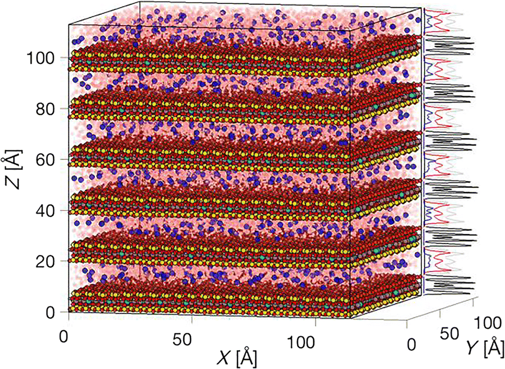
Fig. 2 Example image of a 136,000 particle system generated with the plot_density_atom() function, showing scaled density profiles of a multilayered montmorillonite particle (black profiles), Na+ counter-ions (blue profiles) hydrated by three pseudo-layers of water (Owater in red, Hwater in gray profiles)
Bonding and Structural Analysis
Most functions, such as dist_matrix_atom() and bond_angle_atom(), take PBC into account, which allows for generation of molecular topologies with bonds, angles and basic dihedrals across the PBC. Many functions also support triclinic boxes using the ‘tilt vectors’ xy, xz, yz as defined in Gromacs and LAMMPS. Several of the functions use two types of neighbor cutoffs to find interacting atoms, one shorter cutoff for bonded H’s (default 1.25 Å) and one larger cutoff for all other interactions (default 2.25 Å). Furthermore, a general neighbor-distance analysis can be performed: (1) by comparison with the Revised Shannon radii (Shannon Reference Shannon1976; van Horn Reference van Horn2001); (2) by calculating the bond-valence values using the semi-empirical Bond Valence Method (Brown Reference Brown2009, Reference Brown and Mingos2013, Reference Brown2016) or; (3) by calculating basic XRD profiles. Here, analysis 2 is performed most easily by calling the analyze_atom() function, which first finds all atom bonds and angles to the nearest neighbors. Secondly, it makes educated guesses based on the chemical name and apparent coordination number, the oxidation state, electron configuration, and the ideal crystalline, ionic, and vdW-radii of the atoms. This function is, hence, useful for sanity-checks of either the initial input structures or to scrutinize one simulation result. As the Bond Valence Method also calculates the Global Instability Index (G II), it can further be used in structural data-mining studies to check for structural stress in molecules. As for analysis 3 and XRD analysis, a basic XRD function called XRD_atom() for single-crystal UCs is provided, using 11-coefficient atomic scattering factors (Waasmaier & Kirfel Reference Waasmaier and Kirfel1995).
Trajectory Analysis
Although not the primary purpose of the atom library, support for trajectory reading (and writing) of binary trajectories utilizing the third-party MatDCD or the mxdrfile packages for the .dcd and .xtc|.trr trajectory formats, respectively, is provided (Gullingsrud Reference Gullingsrud2000; Kapla & Lindén Reference Kapla and Lindén2018). For reading .xtc trajectories, one could also use the Gro2mat package (Dien et al. Reference Dien, Deane and Knapp2014). In addition to these third-party binary trajectory packages, text-format trajectories in the .pdb|.xyz|.gro formats are also natively supported by the atom library, where one special version written specifically for the MC code RASPA2 named import_mc_pdb_traj() can handle trajectories with non-constant numbers of atoms.
In order to import a trajectory into MATLAB as shown below, both a coordinate file and a trajectory file is needed.

Apart from the atom struct taken from the coordinate file, this command results in a data matrix called traj, of size 3N×frames, where N represents the number of atoms in the trajectory.
Case Study: A Hydrated Na+-montmorillonite Nanopore System with CLAYFF atomtypes
This example demonstrates the main steps needed to setup a simulation box for MC or MD simulations of a system representing the water–mineral interface to a defect mineral particle called MMT (as in Montmorillonite). MMT will describe a negatively charged smectite layer, with an approximate thickness of 1 nm and being infinite in the lateral plane, due to the fact that PBC is used in MC or MD simulations and because the layer in this example will have no edges in order to avoid complexity.
Preparation of the Mineral Lattice
The negative charge of MMT mainly originates from isomorphic substitution of octahedrally coordinated Al(III) with Mg(II), which creates a charge defect which is smeared over the nearest coordinating O(-II) in the lattice. In most cases when performing molecular modeling of inorganic or mineral particles, initial UC data are available from either X-ray diffraction data or quantum mechanical calculations. For MMT, due to the isomorphic substitution, no precise UC data exist. Instead, one can use isostructural and defect-free UC data from pyrophyllite (Lee & Guggenheim Reference Lee and Guggenheim1981), and then replicate it to a mineral layer and subject it to isomorphic substitution. Hence, initially, a pyrophyllite UC structure must be imported:

In many cases when UC information is taken from XRD data, the number and positions of H atoms are somewhat unreliable. Hence, in this example both initial removal and addition of H atoms to the clay lattice are demonstrated. First, all atoms with names starting with ‘H’ are removed.

Then the remaining mineral lattice is analyzed for the resulting structure using the function analyze_atom().

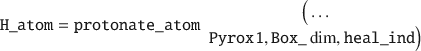
This function will output a separate properties struct with bonding information, as well as reveal which atoms need healing by outputting a heal_ind variable. To protonate those individual atoms, one would issue:
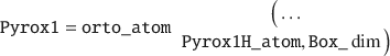
To simplify this example one could convert the triclinic UC to an orthogonal UC:
Next, the UC must be replicated into a layer, for instance by 6×4 times in the X and Y-directions, respectively:
From this pyrophyllite layer, a MMT layer can be generated by performing isomorphic substitution by replacing Al lattice atoms with Mg in two-thirds of all the UCs (which is typical for natural MMT clay minerals). The last numerical argument (in Ångström units) sets the nearest Mg–Mg neighbor distance, as charge defects are unlikely to be close to each other.

For consistency, one can at this point change the attribute MMT.resname from ‘PYR’ to ‘MMT’:
Here, the deal() is a native MATLAB function. Next, the names of all atoms (i.e. the atomtypes) in MMT can be set to a specific forcefield, such as the original CLAYFF (Cygan et al. Reference Cygan, Liang and Kalinichev2004).
This function will also output the layer net charge (–16 from the isomorphic substitution), which must be counterbalanced by counter-cations such as Na+. In order to accommodate these ions and later water molecules, the dimensions of the definitive simulation box should be defined, from the lateral dimensions of the MMT layer along X/Y (already set in the existing Box_dim variable) and an arbitrary height in Z, here set to 40 Å:

Adding Counterions and Solvating with Water
Ions can be added to an existing simulation box in several ways using the ionize_atom() function. In this example, an Ions struct is created by adding ions close to the mineral surface (but >3 Å) of the wrapped MMT:
Note that wrapping the MMT layer into the box before adding the ions is important in order to avoid atomic overlap. Next, a Water struct is created in order to solvate the simulation box. This is accomplished by placing 1000 SPC/E water molecules with a relative density of 1.05 no nearer than 2 Å to any solute:

Finally, all components are merged together using update_atom() into single System struct, which updates all atom- and molecular-ID indexes, and an ouput .pdb file is written. Note that because the different System struct components are stored in separate struct variables, the order of the components can be changed arbitrarily.

The following lines show example commands used to plot the final System struct (see Fig. 3), where, for instance, the optional last numerical in the plot_atom() function denotes the VdW radii scaling factor, whereas the 'vdw' in the show_atom() function sets the display style:

Fig. 3 The final hydrated and unwrapped Na+-MMT System generated by the plot_atom(). Note the legend which indicates the CLAYFF assigned atom types for the Water, Ions, and MMT struct variables. Alternatively, one could plot the System struct or the printed .pdb file with VMD instead.

Writing Molecular Topology Files
The atom library contains different flavors of both the CLAYFF and INTERFACE forcefields. The following examples show how to write basic .psf, .lmp, and .itp topology files according to the original CLAYFF to be used in the MD software like NAMD2, LAMMPS, and Gromacs.

Note that when generating molecular topology files, one must, in general, decide which components to include (i.e. the MMT, Ions, and Water) in the molecular topology, as different MD and MC software may use different approaches on how to include molecular topologies in the total system topology. For instance, in Gromacs, separate molecular topology files are used commonly (.itp files) for different components; hence, the Ions and the Water in the current example would preferably not be included in the same molecular topology as MMT.
On a separate note, because the original CLAYFF (nor INTERFACE) does not contain all different oxygen atom types needed to model all minerals or, for instance, custom clay edge models, the atom library can also be used to derive partial charges and molecular topologies for new oxygen atom types not part of the original CLAYFF forcefield. This is accomplished by equation 1, which in fact can be used to calculate the partial charge of any new or original oxygen atom type in CLAYFF (Tournassat et al. Reference Tournassat, Bourg, Holmboe, Sposito and Steefel2016; Lammers et al. Reference Lammers, Bourg, Okumura, Kolluri, Sposito and Machida2017).
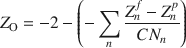
In this equation, the partial charge of a CLAYFF oxygen type (Z O) is obtained from its formal charge (–2) minus the total charge needed to balance (hence the extra minus sign) the charge distributed over all the n nearest coordinating cationic centers (including H). This distributed charge represented by the second term on the right hand side is, in turn, calculated from the difference between the formal and partial charge
 and
and
 of each cation (hence the summation), divided by their respective number of coordinating oxygens, CN
n
. For a more extensive explanation, see Lammers et al. (Reference Lammers, Bourg, Okumura, Kolluri, Sposito and Machida2017).
of each cation (hence the summation), divided by their respective number of coordinating oxygens, CN
n
. For a more extensive explanation, see Lammers et al. (Reference Lammers, Bourg, Okumura, Kolluri, Sposito and Machida2017).
Analyzing the Lattice Structure
In order to study the structural integrity of molecules subjected to molecular simulations, computing the root mean square deviation of atomic positions (RMSD) from the positions in the input structure is an often-used method. This method is frequently used for large biomolecules; however, for crystalline inorganic lattice structures the semi-empirical Bond Valence Method can also be used. This method finds strained atoms in a lattice by relating the so-called bond valence values to the ideal semi-empirical bond distances (Brown Reference Brown2016), as well as by comparing the total bond valence sum to the ideal atomic valence. In this example, this method was applied by invoking the analyze_atom() function on the average MMT lattice structure (Fig. 3) obtained from equilibrated simulations performed in Gromacs in the NVT ensemble over 1 ns. Six different forcefield implementations were tested in total, namely: (1–2) two implementations of the INTERFACE forcefield (Heinz et al. Reference Heinz, Koerner, Anderson, Vaia and Farmer2005, Reference Heinz, Lin, Kishore Mishra and Emami2013), using the experimental or pre-defined bond distance (with the 5% scaling factor) and angle values, respectively; (3) the original unconstrained CLAYFF (Cygan et al. Reference Cygan, Liang and Kalinichev2004), having no defined metal–oxygen bonds or angles; (4) CLAYFF with no bonds but all M–O angle terms defined by the experimental values (as in 1); (5) a modified version of CLAYFF optimized for 1D-XRD modeling, using a larger basal O radius but smaller Si radius (Szczerba & Kalinichev Reference Szczerba and Kalinichev2016); and lastly (6) the same modified version of CLAYFF, but with all angle terms defined as in (4).
The resulting average bond distances (Fig. 4A) from the simulations generally agreed well among the various INTERFACE forcefields, apart from the Mg bond distance for CLAYFF, which was found to relax considerably compared to Al and the INTERFACE forcefields.

Fig. 4 Results from the structural analysis comparing six different implementations of the INTERFACE and CLAYFF forcefields (as explained in the text). (a) Average bond distances for the generic clay lattice atomtypes. (b) The corresponding bond valence sum, compared to the ideal atomic valence, shown as gray lines
Average bond distances reveal little, however, about the strain in lattices. The extended Mg–O bond distances found with the unconstrained CLAYFF but not with the constrained INTERFACE forcefields is reasonable considering the bond valence sum values. This is because a relaxed coordinating octahedron of the neighboring O atoms is needed in order to maintain a physically reasonable atomic valence (+2 for Mg, see Fig. 4B). Nevertheless, the Global instability index, G II, which is a measure of the structural strain for the six different forcefield implementations (1–6) were 0.257, 0.230, 0.366, 0.233, 0.294, and 0.237, respectively. Overall this indicates that the implementations of the forcefields used are not perfect, as G II values >0.2 from experimentally determined structures are found rarely (Brown Reference Brown2009), and hence indicate unstable lattices. Simulations with pyrophyllite (not shown) resulted in similar G II values, which can be compared to the input pyrophyllite structure having a G II value of 0.09. Although the INTERFACE 2013 implementation resulted in the lowest G II value and, hence, the best representation of the internal atomic UC positions, the CLAYFF implementations with defined angles perform almost as well, and are better suited for 1D-XRD modeling due to the larger radius of the basal O atoms (Ferrage et al. Reference Ferrage, Sakharov, Michot, Delville, Bauer and Lanson2011; Szczerba & Kalinichev Reference Szczerba and Kalinichev2016). Still, the radii of the atom types in CLAYFF could likely be further optimized to better represent the bond distances within the actual UC.
DOCUMENTATION
The entire atom library contains >100 unique functions that are summarized in a self-contained html-based documentation, containing explanations for the most common variables and functions and include multiple examples which can be executed interactively from within MATLAB, or be viewed in a browser (also available at moleculargeo.chem.umu.se/codes/atom-scripts). Furthermore, each function describes examples demonstrating all available function arguments.
INSTALLATION
The latest version of the atom library can be downloaded from the MATLAB File Exchange or the GitHub repository github.com/mholmboe/atom. No installation is needed, the library files must only be added to the MATLAB path. Optional use of the visualization program VMD or the MD package Gromacs (which must be installed separately) from within the atom library is possible if the environmental variables in the functions called PATH2VMD() and PATH2GMX() are set. Binary trajectories can be imported with the import_traj function, generating a trajectory matrix and separate Box_dim variable. Supported formats are the .dcd format using the MatDCD script, or the Gromacs formats .trr and .xtc by using mxdrfile (recommended for Gromacs trajectories) or Gro2mat (Gullingsrud Reference Gullingsrud2000; Dien et al. Reference Dien, Deane and Knapp2014; Kapla & Lindén Reference Kapla and Lindén2018).
Conclusions
A flexible MATLAB library for construction and manipulation of molecular models and systems is presented. This atom library contains many useful and time-saving functions that can be used by most researchers with even modest programming experience, in order to setup and perform basic analysis of molecular simulation systems. The main use of the library is to construct custom-made molecular systems and generate topological bonding and angle information across the PBC from the command line, for modeling of geochemical systems such as hydrated clay modeled with the CLAYFF or INTERFACE forcefields in different molecular dynamics or Monte-Carlo simulation packages.
Acknowledgements
Open access funding provided by Umea University. The author acknowledges useful comments by A. Ohlin, and funding from the Faculty of Science and Technology at Umeå University and the Kempe foundation, as well as HPC resources provided by the Swedish National Infrastructure for Computing (SNIC) at High Performance Computing Center North (HPC2N), Umeå University.
Compliance with Ethical Standards
Conflict of Interest
The authors declare that they have no conflict of interest.


 Open access