


1. Introduction
Understanding the mechanisms responsible for transport of a passive scalar, e.g. the temperature field, in a high-speed turbulent flow medium is of fundamental importance for scientific and engineering applications. For example, the turbulent regime is known to enhance the mixing by molecular diffusion in passive scalars where it is the result of a growth in small-scale fluctuations, distortion of scalar interfaces and the occurrence of highly intermittent scalar gradients at small scales of transport (Shraiman & Siggia Reference Shraiman and Siggia2000; Warhaft Reference Warhaft2000; Dimotakis Reference Dimotakis2005; Schumacher, Sreenivasan & Yeung Reference Schumacher, Sreenivasan and Yeung2005). Advancement in understanding of such phenomena is closely dependent on unravelling the complexity that is enforced by the strong nonlinear couplings over a vast range of scales that are also accompanied by the stochastic nature of turbulence (Frisch, Mazzino & Vergassola Reference Frisch, Mazzino and Vergassola1998; Gat, Procaccia & Zeitak Reference Gat, Procaccia and Zeitak1998; Sreenivasan Reference Sreenivasan2019). Therefore, considerable efforts has been devoted to studying the structure of turbulent transport in passive scalars in a scale-space description in the high Reynolds regime (Prasad, Meneveau & Sreenivasan Reference Prasad, Meneveau and Sreenivasan1988; Domaradzki & Rogallo Reference Domaradzki and Rogallo1990), especially by focusing on small-scale intermittency and anisotropy effects (Kang & Meneveau Reference Kang and Meneveau2001; Li & Meneveau Reference Li and Meneveau2006; Watanabe & Gotoh Reference Watanabe and Gotoh2006; Donzis, Yeung & Sreenivasan Reference Donzis, Yeung and Sreenivasan2008; Donzis & Yeung Reference Donzis and Yeung2010; Kitamura Reference Kitamura2021). These efforts originated from the Kolmogorov scale-space description of turbulence (Kolmogorov Reference Kolmogorov1941a,Reference Kolmogorovb) that related the statistics of velocity increments to the average dissipation rate of the turbulent kinetic energy (TKE). Kolmogorov's theory was fundamentally constituted based on a local model for turbulent energy cascade, as demonstrated in Onsager's cascade model for turbulent spectra (Onsager Reference Onsager1945, Reference Onsager1949). This theory was later extended to the turbulent transport of the passive scalars by Obukhov (Reference Obukhov1949), Yaglom (Reference Yaglom1949) and Corrsin (Reference Corrsin1951). Afterwards, the analogy for the different regimes of passive scalar transport given the diffusivity range was developed by Batchelor (Reference Batchelor1959); Batchelor, Howells & Townsend (Reference Batchelor, Howells and Townsend1959).
The initial Kolmogorov theory developed in 1941 was later refined in order to take into account the strong intermittency in the local energy dissipation rate (Kolmogorov Reference Kolmogorov1962; Oboukhov Reference Oboukhov1962). Similarly, highly intermittent fluctuations in the local energy dissipation and also scalar dissipation rates led to the development of refined similarity hypotheses for passive scalars, as presented in Monin & Yaglom (Reference Monin and Yaglom1975).
One of the main pillars of Kolmogorov's theory and its extension to the passive scalars is the local isotropy at small scales. In the case of passive scalar turbulence with large-scale anisotropy (e.g. non-zero mean gradients), it has been shown that the statistics of small-scale scalar fluctuations remain anisotropic (see e.g. Buaria et al. Reference Buaria, Clay, Sreenivasan and Yeung2021) as Pumir & Shraiman (Reference Pumir and Shraiman1995) showed for the case of homogeneous shear turbulent flows. On the other hand, passive scalars are known to exhibit anomalies at the large scales of the turbulent motion such that their effects cannot readily be ruled out with the advection–diffusion (AD) equation (Sreenivasan Reference Sreenivasan2019). According to Warhaft (Reference Warhaft2000), those occur as a result of anomalous mixing arising from rare events in which a parcel of fluid moves a distance much greater than the integral length scale without equilibrating. In the analogy of Lagrangian path integrals, Shraiman & Siggia (Reference Shraiman and Siggia1994) argued that this behaviour is identified for a typical fluid path for which the mixing rate is anomalously long rather than for a typical mixing rate but with an atypical path (Warhaft Reference Warhaft2000). This interpretation is evidence of non-local interactions at the large-scale levels of turbulent motion originating from the presence of anisotropy. According to Warhaft (Reference Warhaft2000), this behaviour is directly linked to the emergence of heavy tails (exponential tails) in the probability density function (PDF) of a passive scalar and has been experimentally observed in the turbulent behaviour of passive scalars with non-zero mean gradient (Gollub et al. Reference Gollub, Clarke, Gharib, Lane and Mesquita1991; Jayesh & Warhaft Reference Jayesh and Warhaft1991, Reference Jayesh and Warhaft1992; Lane et al. Reference Lane, Mesquita, Meyers and Gollub1993). A proper approach to account for a mathematical model representing the accumulative source of these non-local motions is to revisit the spectral transfer model for the cascade of the passive scalar. In fact, this has been a thriving area of research as reported in different studies such as Hill (Reference Hill1978) and Sreenivasan (Reference Sreenivasan1996). A non-local spectral transfer model provides a robust link between the large-scale anisotropy at the energy-containing range and the universal range throughout the turbulent cascade while accounting for the breakdown of local isotropy at small scales.
According to a comprehensive survey by Suzuki et al. (Reference Suzuki, Gulian, Zayernouri and D'Elia2022), fractional-order differential operators provide a promising and predictive direction in mathematical modelling of the non-local behaviour in engineering applications such as mechanics of materials (Suzuki et al. Reference Suzuki, Zayernouri, Bittencourt and Karniadakis2016; Yu, Perdikaris & Karniadakis Reference Yu, Perdikaris and Karniadakis2016; Failla & Zingales Reference Failla and Zingales2020; Suzuki et al. Reference Suzuki, Zhou, D'Elia and Zayernouri2021a,Reference Suzuki, Kharazmi, Varghaei, Naghibolhosseini and Zayernourib,Reference Suzuki, Tuttle, Roccabianca and Zayernouric), modelling the near-wall turbulence (Keith, Khristenko & Wohlmuth Reference Keith, Khristenko and Wohlmuth2021) and Reynolds-averaged Navier–Stokes modelling for wall-bounded turbulent flows (Mehta et al. Reference Mehta, Pang, Song and Karniadakis2019; Song & Karniadakis Reference Song and Karniadakis2021) and subfilter modelling for large-eddy simulation (LES) of turbulence (Samiee, Akhavan-Safaei & Zayernouri Reference Samiee, Akhavan-Safaei and Zayernouri2020; Akhavan-Safaei, Samiee & Zayernouri Reference Akhavan-Safaei, Samiee and Zayernouri2021; Di Leoni et al. Reference Di Leoni, Zaki, Karniadakis and Meneveau2021; Samiee, Akhavan-Safaei & Zayernouri Reference Samiee, Akhavan-Safaei and Zayernouri2022). In particular, LES is known to be an effective technique in computational turbulence research that reduces the computational cost of the simulations by focusing on resolving the larger scales of the transport while the unresolved scales are modelled from the resolved-scale transport quantities (Meneveau & Katz Reference Meneveau and Katz2000; Sagaut Reference Sagaut2006; Moser, Haering & Yalla Reference Moser, Haering and Yalla2021). From a theoretical point of view, the turbulence closure appearing in the LES equations is the result of applying a general filtering operation to the governing equations. In the convolution kernel  $\mathcal {G}_\varDelta (\boldsymbol {x}^\prime -\boldsymbol {x})$ for this filtering operation, $\varDelta$ is considered to be the arbitrary filter size. In LES, the common practice is to take $\varDelta$ large enough towards the intermediate scales of turbulent transport. However, in theory, the filter size could be considered close to the smaller scales of transport ( $\eta$) in a way that $\varDelta \rightarrow \eta$ (Meneveau & Katz Reference Meneveau and Katz2000). With this rationale, one can argue that a ‘well-resolved’ direct numerical simulation (DNS) that is usually resolved up to $2\eta < \varDelta < 5\eta$, may be considered as a candidate for LES with a proper subfilter modelling. Therefore, it is interesting and vital to examine if a developed non-local transport model is reconciled with a non-local subgrid-scale (SGS) model in terms of a priori model identification.
In the present study, we show that using well-resolved standard DNS data for the transport of a passive scalar with uniform mean gradient in a moderately high Reynolds turbulent flow, the three-dimensional (3-D) scalar spectrum does not precisely obey the  $k^{-5/3}$ scaling, where k denotes the Fourier wavenumber, and follows a scaling that is enforced by the large-scale anisotropy. Utilizing Corrsin's generalized cascade model (Corrsin Reference Corrsin1964), we propose a modification to the local time scale associated with the eddies of size $\ell$ as a way to account for the non-local interactions. This modification returns a scaling relation that matches the scalar spectrum after parameterization. Subsequently, the total scalar dissipation is revised and an additional term in the form of a fractional Laplacian of the scalar concentration is obtained. The performance of the AD equation that is equipped with this non-local term is assessed in a seamless DNS setting. The resulting statistical analysis on the fully developed turbulent scalar field shows that considering the effects of non-local interactions in the mathematical model (AD equation) provides a more pronounced prediction of small-scale scalar intermittency along the direction in which the large-scale anisotropy is imposed, and it provides a consistent scaling for the third-order mixed longitudinal structure function over a wide range of scales. Finally, considering the non-local model for the SGS scalar flux proposed in Akhavan-Safaei et al. (Reference Akhavan-Safaei, Samiee and Zayernouri2021), we study the consistency of that fractional-order SGS model (when $\varDelta \approx 2\eta$) with the present non-local modelling for the spectral transfer in scalar turbulence. Our comparison in terms of parameter identification of models shows a perfect reconciliation between the two modelling approaches with less than 1 % difference. The model identification for the SGS model is obtained from the Gaussian process regression (GPR) trained on the high-fidelity filtered DNS data, while the non-local spectral transfer model is calibrated based on the scaling of the 3-D scalar spectrum.
The rest of this work is organized as follows: in § 2, we introduce the mathematical model for the transport of turbulent passive scalars, their spectral transfer view and the non-local modelling for the spectral transfer. In § 3, we provide a detailed statistical analysis for the non-local and standard models in a DNS setting by comparing the single-point, two-point and high-order small-scale statistical quantities. In § 4, the similarities between the current model and the fractional-order subfilter modelling for LES are reconciled. Finally, § 5 provides the concluding remarks.
2. Turbulent transport of passive scalars
The Navier–Stokes (NS) equations that govern incompressible fluid flow dynamics are given by
 \begin{equation} \frac{\partial \boldsymbol{u}}{\partial t} + \boldsymbol{u} \boldsymbol{\cdot} \boldsymbol{\nabla} \boldsymbol{u} ={-}\frac{1}{\rho} \, {\boldsymbol{\nabla}} p + \nu \Delta \boldsymbol{u} + \boldsymbol{F}; \quad \boldsymbol{\nabla} \boldsymbol{\cdot} \boldsymbol{u} = 0, \end{equation}
where  $\boldsymbol {u}$ is the velocity field, $\rho$ denotes the density of fluid, $p$ is the pressure and $\nu$ indicates the kinematic viscosity. Moreover, $\boldsymbol {F}$ represents an external forcing mechanism and in this setting we take it as $\mathcal {A}\boldsymbol {u}$, where $\mathcal {A}$ is a linear indicator function in the spectral domain in order to artificially inject the dissipated TKE into the large scales (low wavenumbers) to generate a statistically stationary isotropic turbulent velocity field (see Akhavan-Safaei & Zayernouri Reference Akhavan-Safaei and Zayernouri2020). In order to model the transport of a conserved passive scalar with the diffusivity ( $\mathcal {D}$) in this medium, the AD equation is a well-known Fickian mathematical model, which is written in the following form:
 \begin{equation} \frac{\partial \varPhi}{\partial t} + \boldsymbol{u} \boldsymbol{\cdot} \boldsymbol{\nabla} \varPhi = \mathcal{D} \Delta \varPhi. \end{equation}
Reynolds decomposition allows for  $\varPhi = \langle \varPhi \rangle + \phi$, where $\langle {\cdot } \rangle$ denotes the ensemble- averaging operator, and $\phi$ is the fluctuating part of the scalar field. In homogeneous turbulence, assumption of a uniform imposed mean gradient, $\boldsymbol {\nabla } \langle \varPhi \rangle = \boldsymbol {G}$, is a common practice in order to consider a forcing mechanism for the turbulent intensity (see e.g. Overholt & Pope Reference Overholt and Pope1996). As a result, (2.2) is rewritten as
 \begin{equation} \frac{\partial \phi}{\partial t} + \boldsymbol{u} \boldsymbol{\cdot} \boldsymbol{\nabla} \phi ={-}\boldsymbol{G} \boldsymbol{\cdot} \boldsymbol{u} + \mathcal{D} \Delta \phi. \end{equation}
The governing equations are numerically solved in the standard pseudo-spectral setting for DNS (Overholt & Pope Reference Overholt and Pope1996; Akhavan-Safaei & Zayernouri Reference Akhavan-Safaei and Zayernouri2020), and the simulation set-up is further explained in § 2.3.
Considering  $E_\phi (k,t)$ as the 3-D scalar spectrum, the spectral budget of the scalar variance reads as
 \begin{equation} \langle \phi^2 \rangle = \int_0^\infty E_\phi(k,t) \, {\rm d}k, \end{equation}
where  $k$ indicates the wavenumber. Through the assumption of small-scale isotropy, the spectral budget for the dissipation rate of scalar variance by molecular diffusion, $\chi$, is given as
 \begin{equation} \chi = 2 \mathcal{D} \int_0^\infty k^2 E_\phi(k,t) \, {\rm d}k. \end{equation}
Depending on the ratio of  $\nu /\mathcal {D}$, and the dissipation rate of TKE ( $\varepsilon$), three main wavenumbers are identified for the scalar spectrum
 \begin{equation} k_{\eta_K} \equiv \left(\frac{\varepsilon}{\nu^3}\right)^{1/4}, \quad k_{\eta_B} \equiv \left(\frac{\varepsilon}{\nu \mathcal{D}^2}\right)^{1/4}, \quad k_{\eta_{OC}} \equiv \left(\frac{\varepsilon}{\mathcal{D}^3}\right)^{1/4}, \end{equation}
associated with the Kolmogorov ( $\eta _K$), Batchelor ( $\eta _B$) and Obukhov–Corrsin ( $\eta _{OC}$) length scales. Unlike the case with Schmidt number $Sc:=\nu /\mathcal {D} \approx 1$ where all of these three wavenumbers are nearly equal, $k_{\eta _B}$ and $k_{\eta _{OC}}$ encode the different behaviours of the scalar spectrum in the presence of the viscous–convective subrange ( $Sc \gg 1$), and inertial–diffusive subrange ( $Sc \ll 1$), respectively. It is convenient to differentiate the scales of turbulent cascade by the wavenumbers $k_{EI}$, $k_{DI}$, as $k < k_{EI}$ represents the energy-containing range, and $k_{EI} < k$ indicates the universal equilibrium range (Pope Reference Pope2001). Moreover, the universal equilibrium range is split into inertial–convective ( $k_{EI} < k < k_{DI}$), and dissipation ( $k_{DI} < k$) subranges for the passive scalars with $Sc=1$ (Hill Reference Hill1978).
2.1. Scalar spectral transfer and modelling
Time evolution for the spectrum of a conserved scalar is governed by (see e.g. Hill Reference Hill1978; Pope Reference Pope2001)
 \begin{equation} \frac{\partial}{\partial t} E_\phi(k,t) - T(k,t) = \mathcal{P}(k,t) - 2 \mathcal{D} k^2 E_\phi(k,t), \end{equation}
where  $\mathcal {P}(k,t)$ denotes the spectral content for the large-scale production rate of the scalar variance, and $T(k,t)$ is the scalar spectral transfer function. The unknown nature of $T(k,t)$ causes a closure problem in (2.7); thus, a proper modelling for the spectral transfer function is required; $T(k,t)$ could be defined as the rate of spectral flux function, $F(k,t)$, per unit wavenumber as (see e.g. Corrsin Reference Corrsin1964; Hill Reference Hill1978)
 \begin{equation} T(k,t) \equiv{-} \frac{\partial F(k,t)}{\partial k}. \end{equation}
By integrating (2.8) over the 3-D spectral domain, the spectral flux function is obtained.
As a well-known assumption,  $\mathcal {P}(k , t)$ mainly contributes to the energy-containing scales directly, while it is obvious that $k^2 E_\phi (k,t)$ is mainly considerable in the small scales of the turbulent cascade where diffusion is the dominant transport mechanism (Pope Reference Pope2001). Therefore, integrating (2.7) over the wavenumber space yields the following:
 \begin{align} \frac{\partial}{\partial t} \langle \phi^2 \rangle &= \int_0^{k_{EI}} \left[\mathcal{P}(k,t)+T(k,t)\right] {\rm d}k + \int_{k_{EI}}^{k_{DI}} T(k,t) \, {\rm d}k \nonumber\\ &\quad + \int_{k_{DI}}^\infty \left[T(k,t) - 2 \mathcal{D} k^2 E_\phi(k,t)\right] {\rm d}k. \end{align}
In the statistically stationary state, the second and third integrals in (2.9) are approximately zero (Hill Reference Hill1978; Pope Reference Pope2001). In other words, within the inertial–convective subrange  $\partial F(k)/\partial k = 0$ by the constant cascade assumption, and for the diffusive subrange $\partial F(k)/\partial k = -2 \mathcal {D} k^2 E_\phi (k)$. As a result, for the wavenumbers in the inertial–convective subrange $F(k) = \chi$, integrating with respect to $k$ and employing (2.5). Subsequently, (2.9) is rewritten as
 \begin{equation} \frac{\partial}{\partial t} \langle \phi^2 \rangle = \underbrace{\mathcal{P}(t)-F(k_{EI},t)}_{\textit{Energy containing}} + \underbrace{\underbrace{F(k_{EI},t) - F(k_{DI},t)}_{\textit{Inertial--convective}} + \underbrace{F(k_{DI},t)-\chi(t)}_{\textit{Dissipation}}}_{\textit{Universal equilibrium range}}. \end{equation}
 This picture motivates the concept of modelling for the turbulent cascade process, here specifically for the case of the scalar transport. This approach was initially introduced by Onsager in Onsager (Reference Onsager1945, Reference Onsager1949), and later was generalized by Corrsin (Reference Corrsin1964) to the cascade mechanism of other systems such as passive scalars. In the cascade transfer, assuming geometric doubling at each wavenumber step would approximate the step length as  $\Delta k \approx k$. Therefore, the spectral flux function could be represented in the following form:
 \begin{equation} F(k) \approx \frac{\textit{scalar variance}}{\textit{unit time}} = \frac{\Delta k E_\phi(k)}{\tau(k)} \approx \frac{k E_\phi(k)}{\tau(k)}, \end{equation}
where  $\tau (k)$ is the time scale associated with the step at wavenumber $k$ (Corrsin Reference Corrsin1964). Within the inertial–convective subrange, choosing $\tau (k)$ to be the local time scale associated with the eddies of size $\ell =k^{-1}$, gives
 \begin{equation} \tau(k) = \left( \frac{[k E(k)]^{1/2}}{1/k}\right)^{{-}1} = \left[k^3 E(k)\right]^{{-}1/2}. \end{equation}
In (2.12),  $E(k)$ is the spectrum of the TKE. Thus, according to the well-known Kolmogorov scaling for the inertial subrange, $E(k) \sim \varepsilon ^{2/3} k^{-5/3}$, where $\varepsilon$ is the dissipation rate of TKE.
Plugging (2.12) into (2.11),  $F(k)= \chi \approx k^{5/2} E(k)^{1/2} E_{\phi }(k)$, and according to the scaling of TKE spectrum, the scalar spectrum scales as
 \begin{equation} E_\phi(k) = \mathcal{C} \chi \varepsilon^{{-}1/3} k^{{-}5/3}, \end{equation}
where  $\mathcal {C}$ is the scaling constant. For a comprehensive overview of a variety of the spectral transfer models as well as the analysis of their dynamics and properties, interested readers are referred to Sagaut & Cambon (Reference Sagaut and Cambon2018, § 4.7.1).
Direct numerical simulation of the scalar turbulence with a uniform imposed mean gradient,  $\boldsymbol {G}=(0,1,0)$, advected on statistically stationary homogeneous isotropic turbulent (HIT) flow, provides a proper database to examine the scaling law in (2.13). In this study, a well-resolved DNS at the Taylor-scale Reynolds number $Re_\lambda =240$ for the case with $Sc=1$ is obtained. Resolving over a sufficiently large time period in the statistically stationary state provides a rich sample space to obtain the ensemble-averaged spectra for the TKE and scalar. Figure 1 illustrates these time-averaged spectra over approximately 15 large-eddy turnover times, $\tau _{ET}$. Although the well-known Kolmogorov scaling for the TKE is achieved, as shown in figure 1(a), figure 1(b) reveals that the scalar spectrum does not obey the scaling law given in (2.13).

Figure 1. Time-averaged 3-D spectra for (a) TKE ( $E(k)$), and (b) turbulent scalar intensity ( $E_{\phi }(k)$), obtained from the DNS results described in § 2.3.
2.2. Non-local modelling of the scalar spectral transfer
In Corrsin's generalization to the Onsager cascade model,  $\partial F/\partial k$ is considered as the rate of gain or loss of the spectral content per unit wavenumber (Corrsin Reference Corrsin1964). Moreover, this generalized model could be applied to:
(i) non-conservative systems;
(ii) systems with different characteristic time scales;
(iii) systems with different cascading mechanisms.
In fact, one can realize that the scaling given in (2.13) was obtained based upon this generalization. However, in the case of a scalar spectrum, a main assumption that might be questioned is small-scale isotropy. Recently, high-fidelity computational studies showed that the effects of large-scale anisotropic forcing do not vanish at the small scales of turbulent transport of passive scalars (see e.g. Buaria et al. Reference Buaria, Clay, Sreenivasan and Yeung2021). Moreover, these small-scale anisotropic fluctuations are identified to be highly intermittent due to the intensified presence of non-local interactions in passive scalar turbulence. Anomalous scaling of high-order scalar structure functions is a clear and well-known experimental evidence supporting this significant deviation from local isotropy at small scales of transport. In fact, these effects are available in the inertial–convective subrange. Accordingly, we also observed that the scaling law for the scalar spectrum has a notable discrepancy from the ensemble-averaged spectrum obtained from DNS.
Based on the Corrsin's generalization, we propose that the effects of the anisotropy could be effectively modelled in the spectral transfer function when the effect of spatial non-locality in the cascade of scalar variance is properly considered. Inclusion of an added power-law behaviour into the eddies of size  $\ell$ mathematically enables modelling of the long-range interactions in the physical domain (spatial non-locality), and would return a modification in the local time scale given in (2.12). As a result, we propose
 \begin{equation} \ell=(k^2+\mathcal{C}_\alpha k^{2\alpha})^{{-}1/2}, \quad \alpha \in (0,1], \end{equation}
where  $\mathcal {C}_\alpha$ is a non-negative model coefficient, and $\mathcal {C}_\alpha = 0$ yields the limit case $\ell = k^{-1}$. Consequently, the modified time scale is derived as
 \begin{equation} \tau(k) = \left[(k^2+\mathcal{C}_\alpha k^{2\alpha}) k E(k)\right]^{{-}1/2}. \end{equation}
Plugging this non-local time scale into (2.11) yields the following modified scaling law:
 \begin{equation} E_\phi(k) = \mathcal{C} \chi \varepsilon^{{-}1/3} k^{{-}2/3} (k^2+\mathcal{C}_\alpha k^{2\alpha})^{{-}1/2}, \end{equation}
and  $\mathcal {C}$ denotes the scaling constant. Testing this modified scaling law on the time-averaged scalar spectrum shows a promising agreement through proper parameterization of $\alpha$ and $\mathcal {C_\alpha }$. In order to parameterize these two values, given the time-averaged 3-D scalar spectrum we obtained from the standard DNS (figure 1b), in the modified scaling law (2.16), we initially set $\mathcal {C}_\alpha = 1$, then vary $\alpha \in (0,1]$. We observe that $\alpha = 0.65$ yields the slope of the time-averaged scalar spectrum; however, the level of the spectral content (for the scalar variance) is achieved when $1< C_\alpha$. Therefore, by fixing the $\alpha =0.65$ and trying incremented realizations of $C_\alpha$ in (2.16), we realize that with $C_\alpha \approx 3.9$ we have reached the desired parameterization. Accordingly, figure 2 illustrates that with this parameterization ( $\alpha = 0.65$ and $\mathcal {C}_\alpha \approx 3.9$) the universal scaling observed in the TKE spectrum is achieved for the scalar spectrum with respect to (2.16).
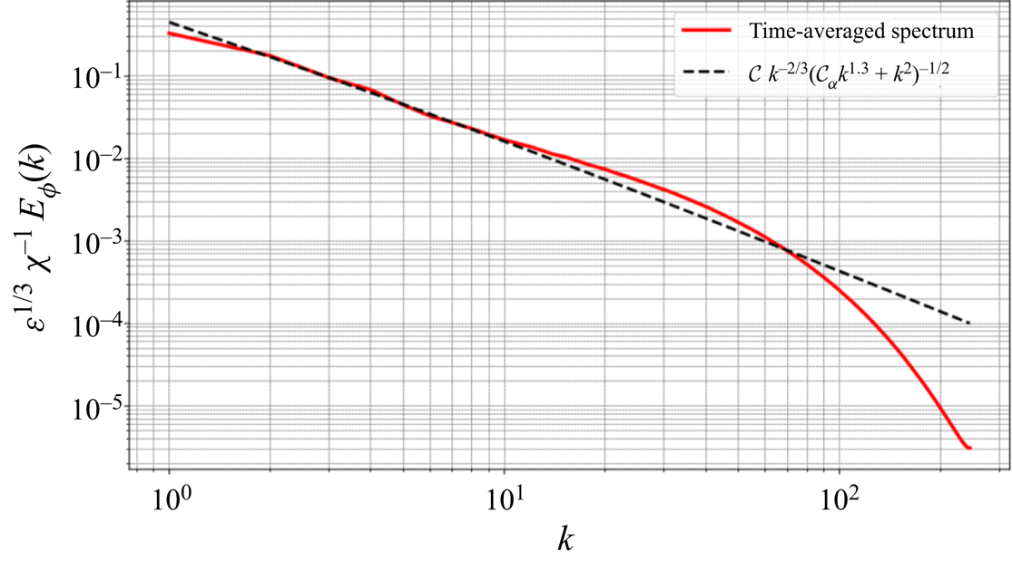
Figure 2. A priori identification of the fractional order and  $\mathcal {C}_\alpha$, for the modified scaling law introduced in (2.16) based upon the calibration of the scaling law with the large-scale content of the time-averaged 3-D scalar spectrum ( $k<10$) that induces the non-locality. The data to compute the scalar spectrum come from the DNS using the standard scalar model. The identified values are $\alpha =0.65$, and $\mathcal {C}_\alpha \approx 3.9$.
The multi-scale nature of the turbulent cascade process implies that the non-local transport effects induced by the large-scale anisotropy are fundamentally connected to the small scales of motion through inter-scale interactions. Here, the inertial–convective subrange essentially plays the role of a meso-scale region for the turbulent cascade, where the presence of these non-local inter-scale interactions is highly pronounced. In fact, several fundamental studies focused on these non-local interactions and tried to unravel their nature by triad and tetrad dynamics models in the spectral domain (see e.g. Waleffe Reference Waleffe1992; Chertkov et al. Reference Chertkov, Falkovich, Kolokolov and Lebedev1995; Chertkov, Pumir & Shraiman Reference Chertkov, Pumir and Shraiman1999; Cheung & Zaki Reference Cheung and Zaki2014; Briard, Gomez & Cambon Reference Briard, Gomez and Cambon2016; Sagaut & Cambon Reference Sagaut and Cambon2018). Therefore, a modification to the dissipation model (2.5) (initiated from the small-scale isotropy hypothesis) would complement the non-local effects observed in larger scales of turbulent cascade. Subsequently, the total dissipation ( $\chi _T$) is revised into
 \begin{align} \chi_T &= 2 \mathcal{D} \int_0^\infty [k^2 + \mathcal{C}_\alpha k^{2\alpha}] E_\phi(k,t) \, {\rm d}k \nonumber\\ &= \underbrace{2 \mathcal{D} \int_0^\infty k^2 E_\phi(k,t) \, {\rm d}k}_{\chi} + \underbrace{2 \mathcal{D} \mathcal{C}_\alpha \int_0^\infty k^{2\alpha} E_\phi(k,t) \,{\rm d}k}_{\chi_\alpha}. \end{align}
Defining  $\mathcal {D}_\alpha := \mathcal {D} \mathcal {C}_\alpha$, $\chi _\alpha$ characterizes the essence of having an underlying non-local diffusion operator in the AD equation governing the turbulent transport of the passive scalar. From a mathematical point of view, $\chi _\alpha$ directly stems from a fractional-order Laplacian operator, $(-\varDelta )^\alpha ({\cdot })$, acting on the scalar concentration; thus, the modified transport model reads as
 \begin{equation} \frac{\partial \phi}{\partial t} + \boldsymbol{u} \boldsymbol{\cdot} \boldsymbol{\nabla} \phi ={-}\boldsymbol{G} \boldsymbol{\cdot} \boldsymbol{u} + \mathcal{D} \Delta \phi + \mathcal{D}_\alpha (-\varDelta)^\alpha \phi. \end{equation}
2.3. Numerical discretization and simulation details
A standard pseudo-spectral scheme based on the Fourier-collocation method is utilized to discretize and resolve the NS and AD equations. The triply periodic computational domain  $\boldsymbol {\varOmega }=[0,2{\rm \pi} ]^3$ is discretized in space by a uniform grid with $520^3$ grid points. A fourth-order Runge–Kutta (RK4) scheme is employed to perform the time integration with a fixed $\Delta t=8\times 10^{-4}$, while the $\text{Courant}{-}\text{Friedrichs}{-}\text{Lewy (CFL)} < 1$ condition is always checked; therefore, numerical stability is ensured. In this study, we select a fully developed HIT field at $Re_\lambda =240$ as the initial state of our computational experiment, and investigate the development of the passive scalar concentration under the effect of a large-scale uniform imposed mean gradient, $\boldsymbol {G}=(0,1,0)$. Concentration field, $\phi (\boldsymbol {x})$, is initiated from zero and is resolved for approximately 30 large-eddy turnover times under the standard model (2.3), and the introduced non-local model (2.18), while $Sc=1$. More detailed discussions about the numerical method, computational approach for the simulations and the flow characteristics of the utilized HIT data have been presented in Akhavan-Safaei & Zayernouri (Reference Akhavan-Safaei and Zayernouri2020).
3. Statistical analysis of the non-local scalar turbulence model
Given the fact that turbulent transport is a stochastic process, sophisticated statistical analysis of the mathematical models for such phenomena has been a centre of attention in turbulence research. In this study, we consider the single- and two-point statistical quantities of interest in passive scalar transport to examine the performance of our non-local modelling within an equilibrium turbulent state against its conventional counterpart.
3.1. Transport of the scalar variance
Transport of the scalar variance provides important information about the evolution of the turbulence intensity. In fact, the computational fluid dynamics approach makes it possible to identify and keep track of the records of different influential mechanisms obtained from the mathematical modelling of the physics. It is well known that multiplying both sides of the AD equation would yield the time evolution equation for the turbulent intensity,  $\phi ^2$. Therefore, applying that to (2.18), after using the incompressibility condition and chain rule for the spatial derivatives, one can derive that
 \begin{align} \frac{1}{2}\frac{\partial \phi^2}{\partial t} &={-} \left[ \boldsymbol{\nabla} \boldsymbol{\cdot} (\boldsymbol{u} \phi^2) - (\boldsymbol{u} \phi)\boldsymbol{\cdot} \boldsymbol{\nabla} \phi \right] - \boldsymbol{G} \boldsymbol{\cdot} (\boldsymbol{u} \phi) \nonumber\\ &\quad + \mathcal{D} \boldsymbol{\nabla} \boldsymbol{\cdot} (\phi \boldsymbol{\nabla} \phi) - \mathcal{D} \boldsymbol{\nabla} \phi \boldsymbol{\cdot} \boldsymbol{\nabla} \phi\nonumber\\ &\quad + \mathcal{D}_\alpha \boldsymbol{\nabla} \boldsymbol{\cdot} \left( \phi \boldsymbol{\mathcal{R}}(-\varDelta)^{\alpha-1/2}\phi \right) - \mathcal{D}_\alpha \boldsymbol{\nabla} \phi \boldsymbol{\cdot} \boldsymbol{\mathcal{R}}(-\varDelta)^{\alpha-1/2}\phi, \end{align}
where  $\boldsymbol {\mathcal {R}}(-\varDelta )^{\alpha -1/2}({\cdot })$ denotes the fractional-order gradient obtained from the Riesz transform (Samiee et al. Reference Samiee, Akhavan-Safaei and Zayernouri2020; Akhavan-Safaei et al. Reference Akhavan-Safaei, Samiee and Zayernouri2021; Samiee et al. Reference Samiee, Akhavan-Safaei and Zayernouri2022). Due to the homogeneity of the scalar fluctuations, averaging over the spatial domain is equivalent to the ensemble-averaging operation $\langle {\cdot } \rangle$ (Pope Reference Pope2001). Thus, applying this averaging operation to (3.1) and considering that homogeneity of the fluctuating fields induces $\langle \boldsymbol {\nabla } \boldsymbol {\cdot} (\boldsymbol {\cdot}) \rangle = \boldsymbol {\nabla } \boldsymbol {\cdot} (\langle \boldsymbol {\cdot} \rangle ) = 0$, the evolution of scalar variance $\langle \phi ^2 \rangle$ is obtained as follows:
 \begin{align} \frac{1}{2}\frac{{\rm d}}{{\rm d}t} \langle\phi^2\rangle = \underbrace{\langle (\boldsymbol{u} \phi)\boldsymbol{\cdot} \boldsymbol{\nabla} \phi \rangle}_{\mathcal{T}} \underbrace{- \langle \boldsymbol{G} \boldsymbol{\cdot} (\boldsymbol{u} \phi) \rangle}_{\mathcal{P}} - \underbrace{\mathcal{D} \langle \boldsymbol{\nabla} \phi \boldsymbol{\cdot} \boldsymbol{\nabla} \phi \rangle}_{\chi} -\underbrace{\mathcal{D}_\alpha \langle \boldsymbol{\nabla} \phi \boldsymbol{\cdot} \boldsymbol{\mathcal{R}}(-\varDelta)^{\alpha-1/2}\phi\rangle}_{\chi_\alpha} . \end{align}
In (3.2), the rate of scalar variance is composed of a balance between the turbulent advection effects ( $\mathcal {T}$), production by the imposed mean gradient ( $\mathcal {P}$), molecular diffusion ( $\chi$) and the non-local diffusion ( $\chi _\alpha$). It is clear that, for the standard scalar transport model in which $\mathcal {D}_\alpha = 0$, the non-local diffusion is consequently zero. According to the simulation considerations described in § 2.3, we collect the records of the contributing terms on the right-hand side of (3.2), and figure 3 illustrates these time records for the standard (figure 3a) and non-local (figure 3b) models. Moreover, during both of the simulations we compute the rate of the scalar variance, ${{\rm d}}/{{\rm d}t}\langle \phi ^2 \rangle$, using a forward-Euler finite difference scheme, and compare it with the record of the right-hand side of (3.2) constructed from the summation of the collected records. For both of the simulations, an excellent match between these two computed quantities is observed during the entire simulation time, as shown in figure 3. In the current work, we are focused on examining the statistical behaviour of the developed non-local model at the ‘turbulence equilibrium’ state. In this context, equilibrium is interpreted when, for the rate of scalar variance, the following condition statistically holds:
 \begin{equation} \frac{\mathcal{P}+\mathcal{T}}{\chi+\chi_\alpha} \sim 1. \end{equation}
Figure 4 displays the record of this quantity for standard and non-local models, and we notice that, after approximately two large-eddy turnover times from resolving the scalar concentration,  $(\mathcal {P}+\mathcal {T})/(\chi +\chi _\alpha )$ starts to fluctuate around 1. In order to make sure that the transient numerical effects are well past, we continue to simulate up to $t/\tau _{ET} = 10$, and consider the rest of the simulation statistics to be in the fully developed turbulence equilibrium state. Therefore, the time-averaging operations in our study are performed on a sample space over $10 \leqslant t/\tau _{ET} \leqslant 30$. Accordingly, we can compute the time-averaged values of the contributing terms in the evolution of the scalar variance given in (3.2) as they are reported in table 1. Comparing the time-averaged values of $\mathcal {P}$ from both of the models reveals that the non-local model approximately includes a 2.5 % higher production rate of the scalar variance by the large-scale scalar mean gradient. A reasonable interpretation for this observation is that, once the non-local transfer of the scalar variance transfer in the cascade process is correctly modelled, this excessive 2.5 % production rate is captured at the equilibrium state for scalar turbulence. In other words, devising a non-local turbulent dissipation model ( $\chi _\alpha$) in the scalar variance cascade mechanism would enable a balance in the equilibrium state so that the non-local effects in turbulent transport originating from the large-scale ‘anisotropy’ source are better captured throughout the DNS.
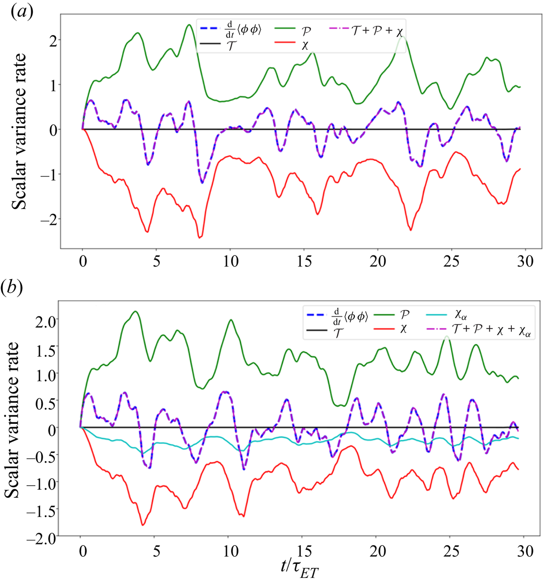
Figure 3. Records of the contributing terms in the time evolution of scalar variance ( ${{\rm d}}/{{\rm d}t}\langle \phi \phi \rangle$) defined on the right-hand side of (3.2), for: (a) standard model, (b) non-local fractional-order model. The time-averaged quantities (over the statistically stationary region of the time records) are reported in table 1.

Figure 4. Tracking the record of the balance in the scalar variance equation ensuring the equilibrium state in simulations of standard and non-local models.
Table 1. Time-averaged values of the contributing terms in the time evolution of scalar variance over the statistically stationary region.

Finally, we compute the time-averaged scalar variance spectrum obtained from the scalar field resolved by the non-local fractional-order model to examine the modified scaling law (2.16) a posteriori. Figure 5 depicts this spectrum and reveals that the scaling (2.16) seamlessly holds. It is worth emphasizing that the total turbulent dissipation is denoted by  $\chi +\chi _\alpha$.

Figure 5. Time-averaged scalar spectrum computed from the data simulated with the non-local model, and evaluation of the identified scaling law in (2.16) for the scalar variance spectrum.
3.2. High-order small-scale statistics of scalar fluctuations
It is well understood that statistics of the turbulence at the small scales of the transport are represented through the central moments of the gradients of the fluctuating fields. Here, we are interested in discovering the small-scale statistics when the scalar field is sufficiently resolved with the proposed non-local scalar transport model. In fact, we seek to understand what the prediction of this model for the asymmetric and highly intermittent nature of passive scalar turbulence at the small scales would be. Therefore, we compute the skewness and flatness factors for the fluctuating concentration gradient, and due to the importance of the statistical behaviour along the anisotropy direction  $\parallel$, we focus on $\mathcal {S}_{\boldsymbol {\nabla }_\parallel \phi }$ and
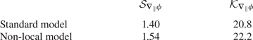
  $\mathcal {K}_{\boldsymbol {\nabla }_\parallel \phi }$. Figure 6 illustrates the records of these two statistical quantities throughout the entire simulation for the standard and non-local models. Over the equilibrium state, explained in § 3.1, we obtain the mean values of the of these statistical quantities by time averaging, and their values are reported in table 2. These time-averaged values show that the non-local model yields a skewness factor 10 % higher than the standard model, and the flatness factor is approximately 7 % higher in the non-local transport model. On the other hand, in a study by Donzis & Yeung (Reference Donzis and Yeung2010) on the resolution effects and scaling in numerical simulations of passive scalar mixing in turbulence, for a similar problem set up at $Re_\lambda = 240$ and $Sc=1$, they performed two sets of standard direct numerical simulations with resolutions (a) $N=512^3$ ( $k_{max} \eta _B \approx 1.5$) and (b) $N=2048^3$ ( $k_{max} \eta _B \approx 5.1$). The resulting high-order statistics we obtained and reported in table 2, are in great agreement with what Donzis & Yeung (Reference Donzis and Yeung2010) reported for the same case in table 4 of their work ( $\mu _3$ and $\mu _4$). In fact, our study shows that our non-local modelling, and the performed DNS based on that, predicts the high-order statistics with approximately 3 % error compared with the extra high-resolution simulation (the case with $k_{max} \eta _B \approx 5.1$) in Donzis & Yeung's study reports. This comparison essentially proves the effectiveness of our modelling while we reduce the computational cost of the simulation approximately 64 times (compared with simulation results with $N=2048^3$ spatial resolution in Donzis & Yeung Reference Donzis and Yeung2010). This evidently implies that an appropriate modelling of the non-local turbulent scalar transfer via the fractional-order model properly reflects the well-known statistical features of highly non-Gaussian behaviour of the passive scalar turbulence reported in the literature (Warhaft Reference Warhaft2000; Sreenivasan Reference Sreenivasan2019).

Figure 6. Time records of (a) skewness, and (b) flatness of the scalar gradient along the anisotropy direction labelled by  $\parallel$. The time-averaged values are identified with dashed lines over the statistically stationary state, and their values are reported in table 2.
Table 2. Time-averaged values of  $\mathcal {S}_{\boldsymbol {\nabla }_\parallel \phi }$, and $\mathcal {K}_{\boldsymbol {\nabla }_\parallel \phi }$ over the statistically stationary state as illustrated in figure 6.
3.3. Two-point statistics and structure functions
Structure functions of order  $n$ for a turbulent field such as the scalar concentration are defined as
 \begin{equation} \langle (\delta_r \phi)^n \rangle = \langle [\phi(\boldsymbol{x}+\boldsymbol{r})-\phi(\boldsymbol{x})]^n \rangle, \quad n>1. \end{equation}
In (3.4),  $\boldsymbol {r}=r\boldsymbol {e}$ where $r$ is the increment of spatial shift, and $\boldsymbol {e}$ denotes a unit vector along a direction of interest. In fact, the structure functions would provide the $n$th-order statistics of spatial increments in the fluctuating field, which are interesting metrics in studying the non-locality. In this study, we are interested in analysing the behaviour of the second- and third-order structure functions of $\phi$ along the direction of large-scale anisotropy, i.e. $\boldsymbol {e}=(0,1,0)$, and regrading the size of the DNS grid, $r=2\eta$. Accordingly, figure 7 shows the time-averaged (over the equilibrium turbulent region) structure functions of orders 2 and 3 obtained from the simulations from standard and non-local scalar transport models. In figure 7(a), one can observe that, for $r>40\eta$, the non-local second-order structure function starts to exhibit higher values compared with the one computed from the simulations using the standard model. For the third-order structure function values, the two models behave similarly up to $r/\eta = 10$; however, after that, the non-local model shows higher values within the spatial shift domain associated with the inertial–convective and integral-scale domain. It is apparent that the maximum value of the time-averaged $\langle (\delta _r \phi )^3 \rangle$ in the non-local model is approximately 10 times higher than the standard model, both occurring at $r/\eta \approx 200$.

Figure 7. Time-averaged  $n$th-order scalar structure functions obtained from the simulations with standard and non-local models, with $r=2 \eta$; (a) $n=2$, and (b) $n=3$.
As initially introduced in Yaglom (Reference Yaglom1949), the mixed ‘velocity-scalar’ third-order structure function is an important two-point statistical quantity measuring the advective turbulent transport in passive scalars. In the presence of large-scale anisotropy (imposed mean scalar gradient), the longitudinal contribution to this mixed structure function plays the dominant role in the advective transport (Iyer & Yeung Reference Iyer and Yeung2014), and its functional form obtained as  $-\langle \delta _r u_L (\delta _r \phi )^2 \rangle$. Here, the subscript $L$ indicates the velocity component along the longitudinal direction with respect to the spatial shift direction $\boldsymbol {r}$, where, in our computational set-up, it would be $u_2$. Similar to the second- and third-order scalar structure functions, we compute a time-averaged value for $-\langle \delta _r u_L (\delta _r \phi )^2 \rangle$ over the stationary time domain. Figure 8 shows that, for the dissipative range ( $r/\eta < 6$), this structure function scales with $r^3$ in both standard and non-local models, while for almost the entire range of $6 < r/\eta < 200$ the mixed structure function obtained from the DNS with the non-local transport model scales with $r^2$. Unlike this universal-range scaling, one can observe that similar behaviour is not necessarily seen in $-\langle \delta _r u_L (\delta _r \phi )^2 \rangle$ when the scalar field is resolved with the standard model. However, in the standard model, a scaling with $r$ could be identified within $20 < r/\eta <60$. This comparison suggests that considering the non-local effects in the turbulent cascade could result in the emergence of more universal behaviour in the two-point statistics of the advective transport, which inherently reveal high-order statistics of the non-locality.

Figure 8. Third-order mixed longitudinal structure function, representing the statistics of advective increments. The non-local model shows a consistent and extended scaling over universal range.
4. Reconciliation with the fractional-order SGS modelling for LES
Recalling § 2.2, we performed an a priori parameter identification that yielded  $\alpha =0.65$ and $\mathcal {D}_\alpha /\mathcal {D} \approx 3.9$ (see figure 2). Here, our goal is to find a consistency between the currently developed model compared with the fractional-order SGS model introduced in Akhavan-Safaei et al. (Reference Akhavan-Safaei, Samiee and Zayernouri2021) when the filter scale is chosen close to the smallest scales of transport. In order to fulfil our goal, we need to show that, given the optimal fractional order for the SGS model as $\alpha _{opt}=0.65$, what is the value of $\mathcal {D}_\alpha /\mathcal {D}$ that is obtained from the procedure introduced in Akhavan-Safaei et al. (Reference Akhavan-Safaei, Samiee and Zayernouri2021) that relies on explicitly filtered data and sparse regression. Taking the filtered data from the simulation based on the standard scalar transport model (2.3) with the time-averaged scalar spectrum shown in figure 2, we can obtain the proportionality coefficient for the fractional-order SGS model. Here, we choose a top-hat box filtering kernel and obtain the filtered data for the filter sizes $\varDelta /\eta =4, 8, 20, 41, 52$. Our goal is to evaluate $\mathcal {D}_\alpha$ when $\varDelta /\eta = 2$; however, it is not computationally possible to obtain the filtered data to infer $\mathcal {D}_\alpha$. Instead, we manage to employ a feasible machine learning algorithm (ML) to predict the desired $\mathcal {D}_\alpha$ while it is trained on the evaluated $\mathcal {D}_\alpha$ values from direct filtered data at larger filter sizes. Gaussian process regression is known to be a suitable ML algorithm when one seeks to predict a quantity of interest from scarce experimental or computationally expensive high-fidelity data. Using the implementation of GPR in the Scikit-Learn package (Pedregosa et al. Reference Pedregosa2011), we obtain the predicted value of $\mathcal {D}_\alpha /\mathcal {D} = 3.87$ for $\varDelta = 2 \eta$ as illustrated in figure 9. This result shows that the a priori estimates for the proportionality coefficient in the non-local scalar transport model are in great agreement with the fractional SGS model when the filter size is selected as $\varDelta = 2 \eta$; therefore, both models are reconciled. It is worth mentioning that the uncertainty in the predictions of the trained GPR for $\varDelta /\eta < 4$ is assessed, and it is observed that the uncertainty is very low and practically negligible (see the 95 % confidence interval in figure 9).

Figure 9. Reconciliation of the non-local model with the fractional-order SGS model developed in Akhavan-Safaei et al. (Reference Akhavan-Safaei, Samiee and Zayernouri2021) when the filter size is assumed to be at the dissipation range of  $\varDelta = 2 \eta$. The value of $\mathcal {D}_\alpha$ is computed from the filtered DNS data for $\varDelta /\eta =4, 8, 20, 41, 52$ based on the data-driven methodology introduced in Akhavan-Safaei et al. (Reference Akhavan-Safaei, Samiee and Zayernouri2021), a GPR is trained based upon these evaluations and $\mathcal {D}_\alpha$ is approximated based on the trained GPR for $\varDelta /\eta < 4$ The predicted $\mathcal {D}_\alpha$ for $\varDelta = 2 \eta$ is found to be in total agreement with the identified one obtained from the scaling analysis a priori in figure 2.
5. Conclusion and remarks
We proposed a modification to the spectral transfer model for the turbulent cascade of passive scalars under the effect of large-scale anisotropy. Employing Corrsin's generalization to Onsager's turbulent cascade model, our modified model introduced an additional power-law term in the definition of the local time scale,  $\tau (k)$, in order to account for the induced non-local contributions originating from the anisotropy sources in the energy-containing range. Subsequently, our approach yielded a modified scaling law for the passive scalar spectrum, $E_\phi (k)$. This modified scaling showed a great match with the time-averaged 3-D scalar spectrum obtained from a well-resolved standard DNS after the parameter identification procedure. Using the integrated equation for the evolution of the scalar spectrum, we revised the total scalar dissipation definition, which introduced an additional term into the total scalar dissipation representing the integrated effects of the non-local turbulent dissipation cascade. This modification to the scalar dissipation returned that a fractional-order Laplacian acting on the scalar concentration is required in the AD equation. Using this revised AD equation, we performed a DNS study to analyse different quantities of turbulent transport compared with the DNS results obtained from convectional model at the statistical equilibrium state. Our analysis on the rate of the scalar variance showed that considering the effects of non-locality in the scalar dissipation results in pronounced prediction of the production rate of scalar variance by the imposed mean gradient (large-scale anisotropy), which could be interpreted as consistency with the breakdown of local isotropy in small scales of passive scalars. On the other hand, we showed that incorporation of the non-locality effects in the scalar dissipation improves the accuracy of predicted time-averaged records of the skewness and flatness factors for $\boldsymbol {\nabla }_{\Vert }\phi$, confirming the essence for devising a proper modelling mechanism for cascade of the anisotropy effects from large to small scales. Moreover, a two-point statistical analysis for the advective scalar increments (the third-order mixed longitudinal structure function) revealed that the DNS results obtained from the non-local model provide a long-range scaling with $r^2$. This observation on long-range scaling suggested that the inclusion of a non-local cascading mechanism in the presence of large-scale anisotropy could result in prediction of more universal behaviour over a wide span of scales in turbulent scalar transport. Finally, we showed an accurate consistency between the developed spectral transfer model and the fractional-order SGS modelling with $\varDelta \approx 2 \eta$, after employing a well-trained GPR model.
Acknowledgements
The authors acknowledge the high-performance computing resources and services that were provided by the Institute for Cyber-Enabled Research (ICER) at Michigan State University.
Funding
This work was financially supported by the ARO YIP award (W911NF-19-1-0444), and partially by the MURI/ARO grant (W911NF-15-1-0562) and the NSF award (DMS-1923201).
Declaration of interests
The authors report no conflict of interest.


 Open access