


1. Introduction
Viscous flows coupled by a deformable solid layer (DS) may be encountered in both natural and engineered processes. In biological systems, such flows occur at the micro-scale, past deformable lipid membranes forming the cell wall and organelles (Fricke Reference Fricke1925; Hochmuth, Mohandas & Blackshear Reference Hochmuth, Mohandas and Blackshear1973; Thaokar & Kumaran Reference Thaokar and Kumaran2002), as well as at a macroscopic level, such as the heart, where the interventricular and interatrial septums act as a DS (Rosenquist et al. Reference Rosenquist, Sweeney, Ruckman and McAllister1979; Marcomichelakis et al. Reference Marcomichelakis, Withers, Newman, O'Brien and Emanuel1983; Pislaru et al. Reference Pislaru, Urban, Pislaru, Kinnick and Greenleaf2014). Engineered systems where such flows are present include membrane separation (Strathmann Reference Strathmann2011) and interfacial polymerisation (Ukrainsky & Ramon Reference Ukrainsky and Ramon2018) processes.
The experiments of Kumaran & Muralikrishnan (Reference Kumaran and Muralikrishnan2000), Srinivas & Kumaran (Reference Srinivas and Kumaran2017), Neelamegam & Shankar (Reference Neelamegam and Shankar2015) and Verma & Kumaran (Reference Verma and Kumaran2012, Reference Verma and Kumaran2013) showed that the presence of a deformable wall in a micro-channel can lead to transitional flows at a much lower Reynolds number compared to rigid-walled channels and, presumably, lead to improved mixing. However, this requires a wall much thicker than the channel dimensions. Furthermore, manipulation of the hydrodynamic instabilities in such a system requires alteration of the fluid and/or deformable wall properties (Verma & Kumaran Reference Verma and Kumaran2012, Reference Verma and Kumaran2013). Thus, during the process, mixing in such a system cannot be actively controlled. Here, we propose that such limitations can be overcome by using a thin, elastic membrane as a DS along with an adjacent, second fluid, as illustrated in figure 1. At any instant during a process, the speed of fluid  $2$ can be used to actively control and trigger hydrodynamic instabilities which in turn can be used to control the mixing in the coupled system. The present theoretical analysis can help in understanding the manipulation of the hydrodynamic instabilities in such systems. Such a system is also representative of some membrane-based separation processes using hollow fibres (e.g. dialysis), essentially a tube whose wall is a permeable, elastic polymer (Strathmann Reference Strathmann2011). This membrane separates two liquid streams flowing at either side. As with the microfluidic system, flow-induced wall vibrations can enhance mixing and intensify the process. Finally, another system of interest is the stability of thin films generated during interfacial polymerisation, commonly used to fabricate desalination membranes (Raaijmakers & Benes Reference Raaijmakers and Benes2016). Here, the ultra-thin polymeric film is formed at a liquid–liquid interface, and its ultimate morphology has been linked to several possible mechanisms, one of which may be of a hydrodynamic origin (Ukrainsky & Ramon Reference Ukrainsky and Ramon2018); the existence of such a mechanism is also part of the motivation to study the stability of this system.

Figure 1. Schematic of the flow geometry in dimensionless coordinates. The plates at  $y=0$ and $y=1+a+b$ are moving with dimensionless speeds $1$ and $V_r$, respectively. The fluids exert a shear stress at the fluid–DS interface, leading to deformation of the DS and coupling between the base-state fluid motion and perturbations in the DS, which affects the stability of the flows.
1.1. Flow past a deformable solid
Before proceeding with the analysis, we begin with an overview of previous studies on related systems. The first study concerning the stability of fluids coupled by a DS was done by Harden & Pleiner (Reference Harden and Pleiner1994), where the DS was treated as an infinitesimally thin elastic sheet. Their study was aimed at explaining experimental studies on dynamic light scattering from insoluble polymeric monolayers at a liquid–liquid interface. Accordingly, the study was focused on hydrodynamic modes induced by thermal fluctuations. As such, their model neglected the governing equations for the solid film. The elastic character of the film affected the liquid–liquid interface only through the tangential stress continuity condition. Other interfacial conditions were those normally applied for a liquid–liquid interface. Additionally, both fluids were static, hence the effect of shear on the membrane and hydrodynamic modes was not studied, in contrast to our present motivation. Kumaran & Srivatsan (Reference Kumaran and Srivatsan1998) added fluid shear and considered the stability of plane Couette flows coupled by a (still) infinitesimally thin DS. Similar to Harden & Pleiner (Reference Harden and Pleiner1994), in their study, the DS was sandwiched between two fluids as shown in figure 1. However, Kumaran & Srivatsan (Reference Kumaran and Srivatsan1998) assumed only normal displacement of the membrane and neglected possible tangential displacement. As a result, a constitutive equation for the DS became unnecessary. Their analysis predicted that in the absence of inertia, the system is stable and the transition Reynolds number is proportional to the dimensionless tension in the thin elastic sheet.
The lack of a constitutive equation in the analysis of Kumaran & Srivatsan (Reference Kumaran and Srivatsan1998) was then relaxed by Thaokar & Kumaran (Reference Thaokar and Kumaran2002), who used a constitutive relation, originally proposed by Harden & Pleiner (Reference Harden and Pleiner1994), for the DS. The flow geometry in Thaokar & Kumaran (Reference Thaokar and Kumaran2002) was similar to the one considered in figure 1. With the added constitutive relation, Thaokar & Kumaran (Reference Thaokar and Kumaran2002) predicted the existence of an instability even in the absence of inertia, in contradistinction with Kumaran & Srivatsan (Reference Kumaran and Srivatsan1998). Thaokar & Kumaran (Reference Thaokar and Kumaran2002) also performed a weakly nonlinear stability analysis and predicted that perturbations in the limit of vanishing wavenumber are supercritically stable. However, similar to Harden & Pleiner (Reference Harden and Pleiner1994) and Kumaran & Srivatsan (Reference Kumaran and Srivatsan1998), Thaokar & Kumaran (Reference Thaokar and Kumaran2002) assumed an infinitesimally thin elastic sheet. As shown later in § 3, their constitutive equation and/or the assumption of infinitesimally thin membrane leads to a seemingly non-physical growth rate in some parametric regimes. This prompted the use of a linear elasticity model and a finite-thickness DS in the present work, consequences of which are discussed in § 3.
1.2. Spatio-temporal stability analysis
The previous studies by Harden & Pleiner (Reference Harden and Pleiner1994), Kumaran & Srivatsan (Reference Kumaran and Srivatsan1998) and Thaokar & Kumaran (Reference Thaokar and Kumaran2002) only considered the temporal evolution of disturbances in the flows coupled by a DS. However, a temporal stability analysis does not provide information about the growth of the disturbances in space or in both space and time simultaneously. This requires a spatio-temporal stability analysis, which may be further classified into either absolute or convective instabilities. A convective instability implies that, given sufficient time, the disturbances will decay at any point in space, while an absolute instability leads to growth of disturbances at any point in space. Further description of both absolute and convective instabilities, as well as an outline of the methodology used to determine their existence, is presented in § 3.2.
An absolute instability has been experimentally observed in several fluid flows, for example, Guillot et al. (Reference Guillot, Colin, Utada and Ajdari2007) and Utada et al. (Reference Utada, Fernandez-Nieves, Gordillo and Weitz2008) observed that an absolute instability leads to jet breakup. The experiments of Lingwood (Reference Lingwood1995) on the boundary layer on a rotating disk showed that the laminar to turbulent flow transition could be a consequence of an absolute instability. In a rotating Hagen–Poiseuille flow, Shrestha et al. (Reference Shrestha, Parras, Del-Pino, Sanmiguel-Rojas and Fernandez-Feria2013) observed the presence of a wavy pattern in the whole tube, presumably due to an absolute instability. Thus, if an absolute instability exists in a given flow geometry, it can bring about dramatic changes. This feature could be exploited in promoting mixing. The length of the system may not be sufficiently large for convective instabilities to grow within the domain of the device. However, if absolute instabilities are present, then the flow is destabilised over the entire domain of the channel, which can enhance mixing, providing further motivation and potentially important practical consequences for probing the existence of absolute instabilities in fluid flows coupled by a DS.
In the present study, linear elasticity is used to model the DS due to the following reasons. For high dimensionless thickness of the DS,  $a$, the study of Gkanis & Kumar (Reference Gkanis and Kumar2003) on the plane Couette flow past a neo-Hookean solid shows that the linear elastic and neo-Hookean models are in excellent agreement. However, at low $a$, for the plane Couette flow past a deformable solid, the critical dimensionless speed of the plates, $\varGamma$, which is proportional to the dimensionless speed of the moving plate, is sufficiently high such that deviations appear in results obtained by linear elasticity, compared with a neo-Hookean model. However, this is not an issue in the present analysis since the coupling instability predicted here for $a<1$ exists at low values of $\varGamma \ (<0.1)$, for which linear elasticity and more advanced models such as the neo-Hookean model are in good agreement (Gkanis & Kumar Reference Gkanis and Kumar2003; Shankar & Kumar Reference Shankar and Kumar2004; Gaurav Shankar Reference Gaurav Shankar2009). Additionally, the linear elasticity model is mathematically and numerically simpler compared to the neo-Hookean model. As shown later in § 3, the linear elastic model removes the unphysical growth rate predicted by the model of Thaokar & Kumaran (Reference Thaokar and Kumaran2002). Therefore, linear elasticity is deemed sufficient to define the dynamics of the DS and hence to study the linear stability of the present system.
The rest of the paper is arranged as follows. The base-state variables and perturbation governing equations are derived in § 2. The temporal stability results and their discussion is given in § 3.1. The existence of the absolute instability and its dependence on the various parameters is discussed in § 3.2. The salient conclusions of the present study are summarised in § 4.
2. Problem formulation
The system under consideration consists of an incompressible, isotropic and homogeneous elastic solid with shear modulus  $G$, sandwiched between two incompressible fluids, as shown in figure 1. The fluids, marked as $1$ and $2$, have viscosities $\mu _1$ and $\mu _2$, respectively and density $\rho$. The densities of the two fluids and the DS are assumed to be equal, which is a reasonable approximation for the industrial processes and biological systems motivating this problem (Hochmuth et al. Reference Hochmuth, Mohandas and Blackshear1973; Strathmann Reference Strathmann2011; Shrestha et al. Reference Shrestha, Parras, Del-Pino, Sanmiguel-Rojas and Fernandez-Feria2013; Pislaru et al. Reference Pislaru, Urban, Pislaru, Kinnick and Greenleaf2014). The lengths in the present problem are scaled by the thickness of fluid $1$,
$1$,  $R$. In the dimensionless coordinates, fluid $1$, DS and fluid $2$ are present in the domains $[0,1]$, $[1,1+a]$ and $[1+a,1+a+b]$, respectively. The length and height of the system are assumed to infinitely extend in the $x$ and $z$-directions. The plates at $y=0$ and $y=1+a+b$ are moving at dimensionless speeds $1$ and $V_r$, respectively, where velocities are scaled by the speed of plate at $y=0$, $V_1$. The parameter $V_r=V_2/V_1$ is the ratio of the plate velocities where $V_2$ is the dimensional velocity of the plate at $y=1+a+b$.
The DS is assumed to be pre-stretched due to the tethering of its ends, in line with practical applications. The tension induced in the DS as a consequence of the tethering is assumed to be much higher than the base state stresses exerted by the flowing fluids. If the DS is un-tethered, then the present analysis is applicable if the interfacial tension is sufficiently large. Otherwise, the fluid shear stress would induce a pressure gradient in the solid that would, in turn, be transmitted to the fluid. Under such conditions, a fully developed Couette flow would no longer be a correct description of the velocity field. A force balance at the fluid–DS interface shows that, for the development of the plane Couette flow for the un-tethered DS, the interfacial tensions must be higher than  $({\varGamma }/{a k^3})(({V_r \mu _r}/{b})+1)$, where $k$ is the wavenumber and $\varGamma$ is the dimensionless speed of the plate at $y=0$. The parameter $\varGamma = \mu _1 V_1/(G R)$ can be interpreted as the ratio of the viscous stresses in fluid $1$ to the elastic stresses within the DS. Another interpretation of $\varGamma$ is the ratio of the relaxation time scale of the DS ( $\sim \mu _1/G$) to the convection time scale ( $\sim R/V_1$). The latter interpretation indicates that $\varGamma$ is a measure of the relative elasticity of the DS. Furthermore, it is assumed that the dimensional widths of each fluid domain, namely $R$ and $bR$, satisfy the condition $R \ll L$ and $bR \ll L$, where $L$ is the length of the DS. This assumption is necessary for using the normal mode analysis employed in the present study. However, if the widths of the fluids and length of the DS are of comparable magnitude, then a fully global stability analysis is required (Theofilis Reference Theofilis2011; Tsigklifis & Lucey Reference Tsigklifis and Lucey2017).
We consider two fluids with a velocity field  $\boldsymbol {v^{(i)}}=(v^{(i)}_x,v^{(i)}_y)$, where $i=1,2$ represent fluids $1$ and $2$, respectively. Scaling the time, $t$, by $R/V_1$, velocities by $V_1$, the dimensionless continuity equation, for an incompressible flow, becomes
 \begin{equation} \boldsymbol{\nabla} \boldsymbol{\cdot} \boldsymbol{v^{(i)}} =0, \end{equation}
where the gradient operator is  $\boldsymbol {\nabla }=\boldsymbol {e}_x ({\partial }/{\partial x})+ \boldsymbol {e}_y ({\partial }/{\partial y})$ with $\boldsymbol {e}_x$ and $\boldsymbol {e}_y$ the unit vectors in the $x$ and $y$-directions, respectively. The dimensionless Navier–Stokes equation for the fluids, with $\mu _1 V_1/R$ used for scaling the pressure, is,
 \begin{equation} Re \left[ \frac{\partial \boldsymbol{v^{(i)}}}{\partial t}+ (\boldsymbol{v^{(i)}} \boldsymbol{\cdot} \boldsymbol{\nabla}) \boldsymbol{v^{(i)}} \right]=-\boldsymbol{\nabla} p^{(i)} +\mu^{(i)} \nabla^{2} \boldsymbol{v^{(i)}}, \end{equation}
where  $Re=\rho V_1 R/\mu _1$ is the Reynolds number. The dimensionless viscosity is $\mu ^{(i)}=1$ for fluid $1$ and $\mu ^{(i)}=\mu _r$ for fluid $2$. Assuming a steady-state and fully developed flow, the base-state velocities of the fluids are
 \begin{gather} \bar v^{(1)}_x =1-y, \end{gather}
 \begin{gather}\bar v^{(2)}_x = \frac{V_r}{b} (y-1-a), \end{gather}
where an overbar indicates a base-state quantity. The subsequent linear stability analysis is performed for this base state.
For the DS, a linear elastic model is used. Scaling the DS displacements by  $R$ and pressure by $\mu _1 V_1/R$, the dimensionless incompressibility and linear momentum equations for the DS are
 \begin{gather} \boldsymbol{\nabla} \boldsymbol{\cdot} \boldsymbol{u}=0, \end{gather}
 \begin{gather}Re \frac{\partial^2 \boldsymbol{u}}{\partial t^2} = -\boldsymbol{\nabla} p_m + \frac{1}{\varGamma} \nabla^{2} \boldsymbol{u}. \end{gather}
Here,  $\boldsymbol {u}=(u_x,u_y)$ is the displacement field in the DS with $u_x$ and $u_y$ the $x$ and $y$ displacement components, respectively, and $p_m$ is the pressure field in the DS.
2.1. Linearised perturbation equations
For the linear stability analysis, two-dimensional disturbances are a reasonable assumption since for the flows past a deformable surface, two-dimensional disturbances have been shown to be more unstable than three-dimensional disturbances (Patne & Shankar Reference Patne and Shankar2018). For the purpose of the linear stability analysis, dynamical quantities such as velocities, displacements and pressures are decomposed into the base state and perturbed state, as  $f(\boldsymbol {x},t)=\bar f(\boldsymbol {x},t)+f'(\boldsymbol {x},t)$. Here, $f(\boldsymbol {x},t)$ is any dynamic quantity and a prime signifies the small perturbation quantity. In the linearised governing equations, the normal modes of the following form are then substituted
 \begin{equation} f'(\boldsymbol{x},t)=\tilde f(y) \exp({\textrm{i} (k x - \omega t)}), \end{equation}
where  $k=k_r+\textrm {i} k_i$ is the complex wavenumber and $\tilde f(y)$ is the eigenfunction of $f'(\boldsymbol {x},t)$. The other parameter, $\omega =\omega _r+ \textrm {i} \omega _i$ is the complex frequency, which characterises the temporal frequency and growth of the disturbances. Therefore, the flow is considered to be temporally unstable if at least one eigenvalue satisfies the condition $\omega _i>0$. For the existence of the spatio-temporal instability, as explained in § 3.2, the cusp point coordinates in the $\omega$ plane must possess $\omega _i >0$. After substitution of the normal modes, the linearised governing equations for the fluid become
 \begin{gather} \textrm{i}k \tilde v^{(i)}_x + D \tilde v^{(i)}_y=0, \end{gather}
 \begin{gather}Re \left[ -\textrm{i}\omega \tilde v^{(i)}_x + \textrm{i} k \bar v^{(i)}_x \tilde v^{(i)}_x + \tilde v^{(i)}_y D \bar v^{(i)}_x \right] = -\textrm{i}k \tilde p^{(i)} + \mu^{(i)} (D^{2}-k^{2}) \tilde v^{(i)}_x, \end{gather}
 \begin{gather}Re \left[ -\textrm{i}\omega \tilde v^{(i)}_y + \textrm{i} k \bar v^{(i)}_x \tilde v^{(i)}_y \right] = -D \tilde p^{(i)} + \mu^{(i)} (D^{2}-k^{2}) \tilde v^{(i)}_y, \end{gather}
where  $D=\textrm {d}/\textrm {d} y$. Similarly, for the DS
 \begin{gather} \textrm{i}k \tilde u_x + D \tilde u_y=0, \end{gather}
 \begin{gather}-\omega^2 Re \tilde u_x = -\textrm{i}k \tilde p_m +\frac{1}{ \varGamma} (D^{2}-k^{2}) \tilde u_x, \end{gather}
 \begin{gather}-\omega^2 Re \tilde u_y = -D \tilde p_m + \frac{1}{ \varGamma}(D^{2}-k^{2}) \tilde u_y. \end{gather}
 The above equations are to be solved using the following boundary conditions. At  $y=0$ and $y=1+a+b$, the assumption of no slip and impermeability of the plates gives
 \begin{gather} \tilde v^{(1)}_x =0;\quad \tilde v^{(1)}_y =0,\quad \textit{at}\ y=0, \end{gather}
 \begin{gather}\tilde v^{(2)}_x =0;\quad \tilde v^{(2)}_y =0, \quad \textit{at}\ y=1+a+b. \end{gather}
 At  $y=1$, oscillations of the fluid–DS interface will be induced due to the perturbations. The perturbed interface is $y=u'_y(\boldsymbol {x},t)|_{y=1}$ so that the linearised normal to the interface is $\boldsymbol {n}^{(1)}=-\boldsymbol {e}_x ({\partial u'_y(\boldsymbol {x},t)|_{y=1}}/{\partial x}) + \boldsymbol {e}_y$, pointing in the positive $y$-direction i.e. from the fluid 1 into the DS, and the tangent is $\boldsymbol {t}^{(1)}=\boldsymbol {e}_y ({\partial u'_y(\boldsymbol {x},t)|_{y=1}}/{\partial x}) + \boldsymbol {e}_x$. There will be four boundary conditions at $y=1$, two of which are continuity of the tangential and normal velocities, while the other two represent continuity of the tangential and normal stresses. These boundary conditions, after substitution of the normal modes, become
 \begin{gather} \tilde v^{(1)}_x+ D \bar v^{(1)}_x \tilde u_y + \textrm{i} \omega \tilde u_x=0, \end{gather}
 \begin{gather}\tilde v^{(1)}_y + \textrm{i} \omega \tilde u_y=0, \end{gather}
 \begin{gather}\textrm{i} k \tilde v^{(1)}_y + D \tilde v^{(1)}_x = \frac{1}{\varGamma}(\textrm{i} k \tilde u_y + D \tilde u_x), \end{gather}
 \begin{gather}-\tilde p^{(1)} + 2 D \tilde v^{(1)}_y = -\tilde p_m + \frac{2}{\varGamma} D \tilde u_y - \varSigma_1 k^{2} \tilde u_y, \end{gather}
where all quantities are evaluated at  $y=1$. The parameter $\varSigma _1$ is the dimensionless interfacial tension between fluid $1$ and the DS. Similarly, for the interface at $y=1+a$, the equation of the surface is $y=-u'_y(\boldsymbol {x},t)|_{y=1+a}$. Thus, the linearised normal and tangent to the fluid–DS interface are $\boldsymbol {n}^{(2)}=\boldsymbol {e}_x ({\partial u'_y(\boldsymbol {x},t)|_{y=1+a}}/{\partial x}) + \boldsymbol {e}_y$ and $\boldsymbol {t}^{(2)}=-\boldsymbol {e}_y ({\partial u'_y(\boldsymbol {x},t)|_{y=1+a}}/{\partial x}) + \boldsymbol {e}_x$, respectively. To maintain consistency with the direction of $\boldsymbol {n}^{(1)}$, $\boldsymbol {n}^{(2)}$ is directed from the fluid 2 into the DS. The boundary conditions at $y=1+a$ are
 \begin{gather} \tilde v^{(2)}_x+ D \bar v^{(2)}_x \tilde u_y + \textrm{i} \omega \tilde u_x=0, \end{gather}
 \begin{gather}\tilde v^{(2)}_y + \textrm{i} \omega \tilde u_y=0, \end{gather}
 \begin{gather}\textrm{i} k \tilde v^{(2)}_y + D \tilde v^{(2)}_x = \frac{1}{\varGamma}(\textrm{i} k \tilde u_y + D \tilde u_x), \end{gather}
 \begin{gather}-\tilde p^{(2)} + 2 D \tilde v^{(2)}_y = -\tilde p_m + \frac{2}{\varGamma} D \tilde u_y + \varSigma_2 k^2 \tilde u_y, \end{gather}
where all quantities are evaluated at  $y=1+a$. Finally, $\varSigma _2$ is the dimensionless interfacial tension between fluid $2$ and the DS.
The term  $D \bar v^{(i)}_x \tilde u_y$ in the tangential velocity continuity conditions at the interface, (2.16) and (2.20), leads to the coupling between the base state and perturbations, which in turn leads to the energy exchange between the DS and the fluids. This energy exchange can eventually lead to the instabilities predicted in the present work. However, we also note that, at higher order, the interaction between the normal interfacial displacement and the pressure fluctuations represents another mode of energy transfer. To determine the stability of the system, the above equations and boundary conditions are solved for the eigenvalue $\omega$ using the numerical methodology outlined in the next subsection.
2.2. Numerical methodology
To carry out the linear stability analysis of the present problem for arbitrary  $Re$, the pseudo-spectral method is employed, in which the eigenfunctions are expanded in terms of Chebyshev polynomials, as
 \begin{equation} \tilde f(y)=\sum_{m=0}^{m=N} a_m T_m (y),\end{equation}
where  $\tilde f(y), m, N, T_m(y)$ and $a_m$ are, respectively, the eigenfunctions, the number of the Chebyshev polynomial, the highest degree of the polynomial in the series expansion or the number of the collocation points, the $m$th Chebyshev polynomial and the coefficient of the latter in the expansion. The series expansions are evaluated at $N$ collocation points to determine the series’ coefficients $a_m$ and/or to obtain the eigenvalues $\omega$. The eigenvalue problem may then be written in the form
 \begin{equation} \boldsymbol{\mathsf{A}}\boldsymbol{e} + \omega \boldsymbol{\mathsf{B}}\boldsymbol{e} + \omega^2 \boldsymbol{\mathsf{C}}\boldsymbol{e}=0, \end{equation}
where  $\boldsymbol{\mathsf{A}},\boldsymbol{\mathsf{B}}$ and $\boldsymbol{\mathsf{C}}$ are the discretised matrices and $\boldsymbol {e}$ is the eigenvector formed by the eigenfunctions of the dynamic quantities such as the velocity, displacements, and the fluid and DS pressures. Next, the polyeig MATLAB routine is used to solve the eigenvalue problem (2.8)–(2.23). To filter out the spurious modes from the numerically computed spectrum of the problem, the latter is obtained for $N$ and $N+2$ collocation points and the eigenvalues are compared with a specified tolerance, e.g. $10^{-4}$. The genuine eigenvalues are verified by increasing the number of collocation points by $20$ and monitoring the variation of the obtained eigenvalues. If the eigenvalue does not change up to the sixth significant digit, then the same number of collocation points are used to predict the critical parameters. In the present work, $N=40$ is found to be sufficient to determine the most unstable converged eigenvalue, within the parameter range studied.
In the creeping-flow limit ( $Re=0$), the governing equations for the fluids and DS can be analytically solved to give eight integration constants. The obtained eigenfunctions for velocities, displacements, as well as the fluid and DS pressures are then substituted into the boundary conditions, resulting in eight equations with eight unknown variables. In matrix form, the resulting eigenvalue problem becomes
 \begin{equation} \boldsymbol{\mathsf{M}} \alpha=0, \end{equation}
where  $\boldsymbol{\mathsf{M}}$ is an $8 \times 8$ matrix containing coefficients of the integration constants and $\boldsymbol {\alpha }$ is a vector containing eight integration constants. The dispersion relation, $\omega =\omega (k,a,b,\varGamma ,\mu _r,V_r,\varSigma _1,\varSigma _2)$ is then obtained by taking the determinant of the matrix $\boldsymbol{\mathsf{M}}$ obtained in the previous step, thereby determining the system stability. In the present work, most of the results are for $Re=0$ and the analytical method does not produce spurious eigenvalues, thus the analytical method is preferred for obtaining results at $Re=0$.
3. Results and discussion
3.1. Temporal stability ( $k_i=0$)

Typical ranges of dimensional parameters involved in flows coupled by a DS, motivating this study, are shown in table 1. According to these, the Reynolds number is estimated to be  $Re \sim 10^{-4} - 1$. Owing to such small value of the Reynolds number, Thaokar & Kumaran (Reference Thaokar and Kumaran2002) assumed the creeping-flow limit in their analysis. Here, we begin with the vanishing $Re$ limit, and separately present the temporal stability results for finite $Re$ in § 3.1.2.
Table 1. Range of dimensional parameters for various physical systems relevant for the current study: membrane separation (MS) (Strathmann Reference Strathmann2011) and interfacial polymerisation (IP) processes (Ukrainsky & Ramon Reference Ukrainsky and Ramon2018), flows near cells (Fricke Reference Fricke1925; Hochmuth et al. Reference Hochmuth, Mohandas and Blackshear1973) and heart (Rosenquist et al. Reference Rosenquist, Sweeney, Ruckman and McAllister1979; Marcomichelakis et al. Reference Marcomichelakis, Withers, Newman, O'Brien and Emanuel1983; Pislaru et al. Reference Pislaru, Urban, Pislaru, Kinnick and Greenleaf2014). Other parameters such as densities and viscosity of the fluids are  ${\sim }10^{3}$ kg m $^{-3}$ and ${\sim }10^{-3} - 10^{-1}$ Pa s, respectively.

3.1.1. Results at $Re=0$

We begin by briefly considering the model presented by Thaokar & Kumaran (Reference Thaokar and Kumaran2002), in which the following relation between the tension ( $T$) and deformation in the DS was assumed,
 \begin{equation} T=K \frac{\partial u_x}{\partial x}, \end{equation}
in the linear limit of a purely elastic DS, where  $K$ is the dimensionless surface modulus of the DS. As shown in figure 2(a), this model predicts a non-physical, unbounded growth rate of the most unstable mode for $V_r=-1$. It must be noted that, Thaokar & Kumaran (Reference Thaokar and Kumaran2002) may not have been able to observe the inconsistent results predicted by their model since a counter-flow arrangement was not studied in their work. The unbounded growth rate shown in figure 2(a) implies some inconsistency in the constitutive equation or assumption of the infinitesimally thin DS. Consequently, in the present work, a linear elastic constitutive equation is employed and a finite thickness of the DS is considered. Figure 2(b) illustrates the removal of the non-physical growth rate for the most unstable (or least stable) mode by the present model, suggesting that considering a finite thickness of the DS and a linearly elastic constitutive equation, resolves the discrepancy. From figure 2(b), the growth rate peaks at $k \sim O(0.1)$, indicating that the dominant disturbances have a wavelength larger than the width of fluid $1$.
$1$.

Figure 2. The variation of the growth rate,  $\omega _i$ with wavenumber, $k$. (a) According to the model employed by Thaokar & Kumaran (Reference Thaokar and Kumaran2002). (b) The present model. The curve for the Thaokar & Kumaran (Reference Thaokar and Kumaran2002) model is obtained at $b=2,\mu _r=0.1,K=50,\varSigma =1$ and $V_r=-1$ while for the present model the parameters are $a=10^{-4},\varGamma =10^{-4},b=2,\mu _r=0.5,\varSigma _1=1$ and $\varSigma _2=1$. $\omega _i>0$ implies an unstable eigenmode. The present model does not predict the unbounded (non-physical) growth rate. (a) Thaokar & Kumaran (Reference Thaokar and Kumaran2002) model and (b) present model.
In the creeping-flow limit, the present analysis predicts four eigenvalues, shown in table 2. The instability predicted herein is due to the first eigenvalue in the table, which is a downstream travelling mode that remains downstream within the parameter range studied (‘downstream mode’ and ‘upstream mode’ here implies disturbances having positive and negative  $\omega _r$, respectively). Hence, this mode is the focus of the forthcoming discussion. The remaining three modes are always stable.
Table 2. Typical eigenspectrum in the creeping-flow limit at  $k=0.5, a=10^{-4}, \varGamma =10^{-4}, b=2$, $\mu _r=0.5, V_r=0, \varSigma _1=1$ and $\varSigma _2=1$. The unstable mode ( $\omega _i >0$) signifies the instability. The other three modes always remain stable.

The form of the perturbations for the unstable eigenmode, at marginally stable parameter values, is shown in figure 3, normalised by the maximum absolute value of the corresponding eigenfunctions. In figure 3(a), at  $y=0$, $v'^{(1)}_x$ vanishes, as required by the boundary conditions at the moving plate near fluid $1$. This is likewise observed for $v'^{(2)}_x$, where the disturbances must vanish at $y=1+a+b$, which corresponds to $y=1$ in figure 3(c). Interestingly, the absolute values achieved by the normalised perturbations $v'^{(1)}_x$ and $v'^{(2)}_x$ at the fluids–DS interface are equal. Consequently, the DS exhibits anti-symmetric oscillations (figure 3b). Thus, the unstable mode predicted in the present work is anti-symmetric in nature.

Figure 3. The normalised perturbations, for the fluids and DS, at  $a=0.6,b=1,\varGamma =0.57,\mu _r=0.5,k=0.029,\varSigma _1=1,\varSigma _2=1$ and $V_r=0$ for the marginally stable eigenvalue $\omega =0.01001$. Here, $v'^{(1)}_x=Re[ \tilde v^{(1)}_x \,\textrm {e}^{\textrm {i}kx} ],v'^{(2)}_x=Re[ \tilde v^{(2)}_x \,\textrm {e}^{\textrm {i}kx} ]$ and $u'_{x}=Re[ \tilde u_{x} \,\textrm {e}^{\textrm {i}kx} ]$. For convenience, the axes for the fluids and DS have been normalised to the interval $[0,1]$. The length of the domain in the $x$-direction is equal to a wavelength ( $2{\rm \pi} /k$) of the perturbations. The plots show that the unstable eigenmode is antisymmetric. (a) $v'^{(1)}_x$; (b) $u'_{x}$; and (c) $v'^{(2)}_x$.
The oscillations of the DS, in the perturbed state, are shown in figure 3(b). Figure 4 shows that the second mode is symmetric with respect to the horizontal perturbation displacement of the DS, while the oscillations of the DS for the third and fourth modes are almost identical except that the fourth mode exhibits tilted oscillations. Interestingly, the oscillations for both the third and fourth modes exhibit slight variations in  $x$ and $y$.
$y$.

Figure 4. The normalised horizontal perturbation displacement of the DS for the remaining three modes at  $a=0.6,b=1,\varGamma =0.57,\mu _r=0.5,k=0.029,\varSigma _1=1,\varSigma _2=1$ and $V_r=0$. Panels (a–c) are for the second, third and fourth modes, respectively, which are all stable. The designations first, second, third and fourth modes refer to the number of the mode when the eigenvalues arranged in the descending order of the imaginary part similar to table 2.
In a typical experiment aimed at detecting hydrodynamic instabilities, the growth of disturbances is observed as a function of the slowly increasing velocity. In the present study,  $\varGamma$ is the dimensionless speed of the plate and also a measure of the shear stress applied by the flow on the DS. Therefore, we study the variation of the critical value of $\varGamma$ ( $\varGamma _c$), as affected by different model parameters, as an indicator of system stability. To estimate the critical parameters, neutral stability curves are obtained, as illustrated in figure 5, for two values of $a$, the dimensional thickness of the DS, and fixed values of the other parameters. The minimum in the neutral stability curve corresponds to the values of the critical wavenumber, $k_c$ and $\varGamma _c$. For $a=10$, in figure 5, the neutral stability curve is flatter compared with the one for $a=0.125$. Physically, this implies that at the critical speed of the plate, for $a=10$, disturbances with a broader wavenumber range will become unstable. Neutral stability curves also show that with a decrease in $a$,
$a$,  $\varGamma _c$ decreases, demonstrating a destabilising effect when the thickness of the DS is decreased.

Figure 5. The neutral stability curves in  $k-\varGamma$ space at $b=1,\mu _r=0.5,V_r=-1,\varSigma _1=1$ and $\varSigma _2=1$. The critical parameters, $k_c$ and $\varGamma _c$, decrease with decreasing $a$. The neutral stability curve for $a=10$ is flatter compared to the one for $a=0.125$ showing that for the critical parameters, a broad range of unstable disturbances can be observed for $a=10$.
The critical wavenumber,  $k_c$, and $\varGamma _c$, obtained from neutral stability curves calculated for various values of $a$, are plotted in figure 6. The figure shows a non-monotonic variation in both $k_c$ and $\varGamma _c$ with a decrease in $a$. Evidently, a decreasing thickness of the DS leads to the lowering of the instability threshold and the wavelength of the unstable disturbances increases. Figure 6 also shows the existence of an unconditionally unstable region for $a<0.12$. This region is characterised by the absence of well-defined critical parameters.

Figure 6. The variation of  $k_c$ and $\varGamma _c$ with $a$ at $b=1,\mu _r=0.5,V_r=-1,\varSigma _1=1$ and $\varSigma _2=1$. The stable region exists on the concave side of the $\varGamma _c$ curve. The steep decrease in $\varGamma _c$ as $a \rightarrow 0.1$ indicates the existence of an unconditional instability for ${a<0.12}$. The unconditionally unstable region arises due to the terms in the tangential velocity continuity equations (2.16) and (2.20), which introduce a coupling between the fluids via the DS at low $a$.
$a$.
For higher values of  $a$, the curve for $\varGamma _c$ becomes akin to the problem of the plane Couette flow past a plate lined by a DS (Kumaran, Fredrickson & Pincus Reference Kumaran, Fredrickson and Pincus1994), and $\varGamma _c$ decreases with increasing $a$. The plane Couette flow past a plate lined by a DS exhibits a ‘viscous mode’ of instability in the creeping-flow limit (Kumaran et al. Reference Kumaran, Fredrickson and Pincus1994; Gkanis & Kumar Reference Gkanis and Kumar2003, Reference Gkanis and Kumar2005). We recall that the present system differs from the one studied by Kumaran et al. (Reference Kumaran, Fredrickson and Pincus1994) through the existence of the second fluid. Considering the variation of $\varGamma _c$ with $a$ shown in figure 6, the instability is similar to the viscous mode for higher $a$. However, as $a$ is decreased, the viscous mode of the instability is affected by the coupling with the second fluid, which leads to a rapid decrease in the critical parameters, as shown in figure 6. To conclude, the flow geometry considered here exhibits an instability similar to the viscous instability at high $a$; however, at low $a$, the coupling between the fluids via the DS modifies the viscous instability and results in an unconditionally unstable region.
Earlier studies in the creeping-flow limit, by Kumaran et al. (Reference Kumaran, Fredrickson and Pincus1994) and Gkanis & Kumar (Reference Gkanis and Kumar2003), concluded that the viscous instability was due to the amplification of the disturbances at the interface between the fluid and DS. These are driven by the interaction term between the base-state velocity gradient and the perturbation in the vertical displacement of the DS, in the tangential velocity continuity equations (2.16) and (2.20). This interaction term couples the base state and perturbations, facilitating the transfer of energy from the base state to the perturbations. Further analysis reveals that the interaction terms in the tangential velocity continuity equations (2.16) and (2.20), are also the reason for the unconditionally unstable region predicted in figure 6, as shown in table 3. The existence of the unconditionally unstable region implies that as long as there is a non-zero deformation (i.e.  $\varGamma \neq 0$) in the DS due to the shear applied by the flow past the interface, then the coupled system is always linearly unstable provided that $a$ and $\mu _r$ are sufficiently small. Furthermore, as illustrated in table 3, this is due to the energy exchange occurring at the fluids–DS interface through $D \bar v^{(i)}_x \tilde u_y$ terms in the tangential velocity continuity equations (2.16) and (2.20). We further note that, for a rigid solid, the deformation is absent, thus $\tilde u_x = \tilde u_y=0$, which removes the $D \bar v^{(i)}_x \tilde u_y$ terms in the tangential velocity continuity equations (2.16) and (2.20), eliminating the instability. Interestingly, from table 3, the decay rate of the second (stable) eigenvalue is less affected by the absence of the terms $D \bar v^{(i)}_x \tilde u_y$, compared to the unstable eigenvalue, while the decay rates of the remaining two eigenvalues remain unaffected even after removal of the interaction terms ( $D \bar v^{(i)}_x \tilde u_y$). This implies that the unstable mode is destabilised due to the energy exchange at the fluid–DS interface while other modes remain unaffected or are very weakly affected.
Table 3. The eigenspectrum with/without the  $D \bar v^{(i)}_x \tilde u_y$ terms in the tangential velocity continuity equations (2.16) and (2.20). The eigenvalues are obtained at $k=0.05, a=10^{-4}, \varGamma =10^{-5}, b=2$, $\mu _r=0.5, V_r=0, \varSigma _1=1$ and $\varSigma _2=1$. The table shows that $D \bar v^{(i)}_x \tilde u_y$ terms are responsible for the unconditionally unstable region, as these terms couple the base state with the perturbations.

The role of  $\mu _r$ in the unconditionally unstable region is shown in figure 7(a). In contrast to the case of high $a$, for sufficiently low $a$ the coupling established between the fluids through the DS is strong enough to make the coupled system unstable at non-zero $\varGamma$. However, the unconditionally unstable region comes at the ‘price’ of a low growth rate at low $\varGamma$, which will be further discussed in the subsequent section.

Figure 7. The effect of varying the viscosity ratio,  $\mu _r$ (a), the relative velocity of plate $2$,
$2$,  $V_r$ (b) and the dimensionless thickness of fluid $2$,
$2$,  $b$ (c) on the curves in $\varGamma _c-a$ parametric space at $\varSigma _1=1$ and $\varSigma _2=1$. Panel (a) shows that a lowered viscosity of fluid $2$ compared to fluid $1$ is favourable for the instability to set in. Panel (b) shows that co-flow is more unstable than counter-flow. Panel (c) illustrates the destabilising effect of an increased thickness of fluid $2$,
$2$,  $b$. Panel (d) shows the rapidly decreasing growth rate with decreasing $k$ and/or $\varGamma$. (a) Varying $\mu _r$ at $V_r=0,b=1$; (b) varying $V_r$ at $\mu _r=0.5,b=1$; (c) varying $b$ at $\mu _r=0.5,V_r=0$ and (d) $\omega _i$ vs $\varGamma$ at $a=10^{-4},b=1,\mu _r=0.5,V_r=0$.
The important role of fluid  $2$ in the induced instabilities can be illustrated with the help of figure 7(c). For $b=0.1$, the $\varGamma _c$ curve is very similar to the curve for a Couette flow past an elastic solid, since $\varGamma _c$ decreases with increasing $a$. This implies that a minimum thickness of fluid $2$ is necessary for the destabilising coupling between the two fluids via the DS. For $b=1$, this requirement is fulfilled and the coupling has a strong effect on the viscous mode instability. Furthermore, increasing $b$ leads to an increase in the minimum value of $a$, at which point the system becomes unconditionally unstable.
Figure 7(b) illustrates the effect of the variation in  $V_r$, which represents the shear force acting on fluid $2$, compared to fluid $1$. The figure shows that the co-flow configuration is more unstable than counter-flow. As explained in the preceding discussion, the terms $D \bar v^{(i)}_x \tilde u_y$ in the tangential velocity continuity equations (2.16) and (2.20) are the main cause of the instability predicted in the present work. The influence of the coupling terms increases with an increase in the DS deformation, which is, in turn, induced by the shear force exerted by the flow. In the counter-flow configuration, the shear force acting on the DS due to both fluids is in the opposite direction, reducing the deformation in the DS and, hence, stabilising the disturbances. Conversely, under co-flow, the shear forces exerted by the fluids reinforce each other, increasing the coupling and resulting in de-stabilisation. The effect of varying the viscosity ratio, $\mu _r=\mu _2/\mu _1$ on the critical parameters is shown in figure 7(a). For $\mu _r=1$, the unconditionally unstable region does not exist, suggesting a strongly stabilising effect imparted by the viscosity of fluid $2$. Through computations of similar $\varGamma _c$ curves for various values of $\mu _r$ in the range $[0.5,1]$, the critical value of $\mu _r$ was found to be $\sim 0.98$ for the existence of the unconditionally unstable region. Furthermore, the curve corresponding to $\mu _r = 0.75$ illustrates that an increase in viscosity of fluid 2 can push the unconditionally unstable region to lower values of $a$.
$a$.
Figures 7(a), 7(b) and 7(c) also show that in certain parametric regimes,  $\varGamma _c \sim O(1)$ for which the linear elastic model is not applicable (Gaurav Shankar Reference Gaurav Shankar2009, Reference Gaurav Shankar2010; Patne & Shankar Reference Patne and Shankar2018). Instead, a material frame-invariant model such as the neo-Hookean or Mooney–Rivlin model is applicable. However, in applications such a high value of $\varGamma$ is not realisable owing to the practical and application restrictions. The results for such a high $\varGamma$ have been presented here only for the sake of completion.
In figures 6, 7(a), 7(b) and 7(c), the system is unstable for any non-zero value of  $\varGamma$ and $k_c \rightarrow 0$. However, for such an unconditionally unstable region, the growth rate of the disturbances also decreases with decreasing $k$ and $\varGamma$, as illustrated in figure 7(d). Owing to the small growth rate, this regime of the instability may not actually be observable experimentally. We note that the low $a$ regime may be relevant in processes involving thin elastic films such as membranes or lipid bilayers. Furthermore, to induce mixing in a practical setting, the growth rate should be high, such that it may lead to the rapid movement of fluid particles (Verma & Kumaran Reference Verma and Kumaran2012, Reference Verma and Kumaran2013; Bodiguel et al. Reference Bodiguel, Beaumont, Machado, Martinie, Kellay and Colin2015). Figure 7(d) shows that, for $k=0.005$ and $\varGamma =10^{-10}$, the characteristic growth time of the disturbances is ${\sim }10^{7}\ \textrm {s}$, while for $k=0.5$ and $\varGamma =10^{-4}$, it is ${\sim }10^{2}\ \textrm {s}$, which is realistically achievable experimentally and in practice. In applications, owing to the practical constraints, the length of the DS will be restricted. Accordingly, for a DS of length $L$, the smallest disturbance wavenumber would be $2{\rm \pi} /L$.
An estimate to observe the coupling instability predicted here in the experiments or practical applications can be obtained as follows. Consider the membrane separation process for which the dimensionless parameters from table 1 are  $a \sim O(10^{-3}-10^{-6}), b \sim O(10^{-3}-10^{-6}), V_r \sim O(0-10)$ and $\mu _r \sim O(0.1-10)$. To detect the coupling mode instability, assume $\mu _r \sim 0.5$ and $V_r=0$ so that the figure 7(d) can be readily used. Then the instability exists for $k<0.9$ and arbitrary $\varGamma$ values. For membrane separation processes, length $L \sim O(10^{-2}-10)\ \textrm {m}$. Thus, depending on $L$, the minimum $k$ will be selected by the system. For example, if $L \sim O(1)$, then from figure 7(d), the temporal coupling instability will exhibit a growth rate of $O(10^{-2})\ \textrm {s}^{-1}$ which is possible to be observed in the experiments. Also, the dimensionless speed of the plate needed to destabilise the disturbances having $k \sim 0.8$ is $\varGamma \sim 10^{-4}$ which corresponds to $V_1 \sim 10^{-2}-10^{-4}\ \textrm {m}\ \textrm {s}^{-1}$, for a membrane of shear modulus $G \sim 10^{5}\ \textrm {Pa}$ and channel height $R \sim 10^{-4} - 10^{-6}\ \textrm {m}$ which again falls within a practical parametric regime. Please note that, if the interfacial tension is sufficiently small, then the coupling instability predicted here can exist for $k>1$, in which case the minimum $L$ required to observe instability can become as low as $\sim \! 0.1$.
Further analysis at  $k \rightarrow 0$ reveals that, for any given combination of the parameters, $k_c \neq 0$ since for $k \rightarrow 0$, only one non-trivial eigenvalue exists,
 \begin{equation} \omega=-\frac{b+\mu_r}{a \varGamma \mu_r}i, \end{equation}
which is unconditionally stable. To conclude, for the low  $a$ regime, despite exhibiting instability at small $k$ and $\varGamma$, due to practical restrictions and small growth rate, such instability may not be of physical relevance. However, the same instability might play a significant role in inducing mixing at sufficiently high $k$ and $\varGamma$.
3.1.2. Instability characteristics at finite $Re$

The results discussed in § 3.1.1 are for a vanishing Reynolds number,  $Re$. However, physical restrictions dictate that $Re$ may be small but of a finite value. Furthermore, the previous study of Thaokar & Kumaran (Reference Thaokar and Kumaran2002) only considered the creeping-flow limit in their analysis, neglecting the influence of inertia on the instability. Motivated by these two reasons, the effect of the variation in $Re$ on the instabilities is studied in the present section.
In the creeping-flow limit, as shown in table 2, only four eigenvalues exist for arbitrary values of the parameters. However, for non-zero  $Re$ there is an unlimited number of eigenvalues, dependent on the number of collocation points used to discretise the differential operator. For $N=40$ collocation points, the eigenspectrum is shown in figure 8. The eigenvalues, other than those present in the creeping-flow limit, are the shear waves generated at the fluid–DS interfaces. Interestingly, these shear waves are stable for $Re<1$. For $Re>1$, these waves may give rise to multiple unstable modes (Gaurav Shankar Reference Gaurav Shankar2009, Reference Gaurav Shankar2010; Patne & Shankar Reference Patne and Shankar2018). In the present system, as discussed in § 3.1.1, $Re<1$, thus shear waves are found to be stable. This implies that, unlike in the viscous mode, the shear waves remain unaffected by the presence of fluid $2$ at low $Re$. As a consequence of the stability of the shear waves for $Re<1$, the viscous mode determines the stability of the system even in the presence of finite inertia. Figure 9 illustrates the effect of the increase in $Re$ on the critical parameters. Increasing inertia has a slightly stabilising effect on the viscous mode. Thus, the results presented for $Re=0$ in § 3.1.1 are generally applicable for $Re<1$, with a minor quantitative adjustment.

Figure 8. The eigenvalue spectrum at  $Re=0.1,a=0.1,b=1,\mu _r=0.5,V_r=0,\varGamma =0.05, k=0.05, \varSigma _1=1$ and $\varSigma _2=1$. The shear waves arising due to the interaction of the fluids and DS are symmetrically distributed about $\omega _r=0$ line. The unstable viscous mode of instability, $\omega =0.013500 + 0.000727i$ is located on the symmetry line of the spectrum.

Figure 9. The variation of  $\varGamma _c$ and $k_c$ with $Re$ at $a=0.6,b=1,\mu _r=0.5,V_r=0, \varSigma _1=1$ and $\varSigma _2=1$. The figure illustrates the stabilising effect of inertia on the viscous instability. The viscous instability remains the dominant mode of instability for $Re<1$.
3.2. Spatio-temporal stability analysis ($k_i \neq 0$) at $Re=0$


When performing a temporal stability analysis (see § 3.1), the frequency of the disturbances,  $\omega$, is taken as a complex number and the wavenumber, $k$, is a real number (Drazin & Reid Reference Drazin and Reid1981). Conversely, for a spatial stability analysis, used to study the evolution of disturbances in space, $\omega$ is taken as a real number and $k$ as a complex number (Drazin Reference Drazin2002). In a spatio-temporal stability analysis, both $\omega$ and $k$ are treated as complex numbers (Huerre & Monkewitz Reference Huerre and Monkewitz1990; Schmid & Henningson Reference Schmid and Henningson2001) and instability is classified as either an absolute or convective instability. This section is aimed at understanding the effect of the fluid–solid coupling on the spatio-temporal instabilities, in the creeping-flow limit.
The classification of flows as absolutely or convectively unstable was first proposed by Briggs (Reference Briggs1964) in the context of plasma physics. He further developed the methodology to investigate the spatio-temporal instabilities by progressive moving of the Laplacian contour in the complex frequency plane and Fourier contour in the wavenumber plane. According to Briggs (Reference Briggs1964), absolute instability signifies the growth of disturbances in both upstream and downstream directions, while convective instability implies that the disturbances develop in the downstream direction from the source of the disturbances. Thus, convective instability will decay at any fixed position in space if provided sufficient time (Huerre & Monkewitz Reference Huerre and Monkewitz1990), resulting in mixing only in the downstream direction, while absolute instability will induce mixing both up- and downstream. This can be illustrated by considering the response of a given base velocity profile to an impulse excitation at asymptotically long times (Huerre & Monkewitz Reference Huerre and Monkewitz1990), where the obtained response is used to determine whether the flow is absolutely or convectively unstable.
The absolute instability is absent in a plane Couette flow past a rigid surface since the flow is temporally stable (Drazin Reference Drazin2002) – for the existence of an absolute or convective instability, the flow must be temporally unstable (Huerre & Monkewitz Reference Huerre and Monkewitz1990; Schmid & Henningson Reference Schmid and Henningson2001). However, the plane Couette flow past a plate lined by a DS exhibits an absolute instability since the fluid–DS coupling gives rise to the temporal instability (Patne & Shankar Reference Patne and Shankar2017). The present flow geometry also possesses a deformable boundary but it differs from the plane Couette flow past a DS due to the presence of fluid  $2$, which may lead to modification of the results predicted by Patne & Shankar (Reference Patne and Shankar2017). The assumption of creeping flow in the present section is due to the considerable simplification in the numerical determination of the saddle and cusp points. Also, as shown in § 3.1.2, $Re$ has a negligible effect on the instabilities for $Re<1$.
To illustrate the absolute and convective instabilities, consider a dispersion relation of the form  $\omega =f(k)$, where $f(k)$ is a continuous and differentiable function of $k$. For the absolute instability to exist, the group velocity of the disturbances must vanish for at least one value of $k$, so that ${\partial \omega }/{\partial k}=0$ (Huerre & Monkewitz Reference Huerre and Monkewitz1990; Schmid & Henningson Reference Schmid and Henningson2001). However, the determined saddle point must also obey the causality principle for the existence of the absolute instability (Huerre & Monkewitz Reference Huerre and Monkewitz1990). To obtain the sufficient condition, equation ${\partial \omega }/{\partial k}=0$ is solved for $k$, which gives the saddle points of the dispersion relation. If the saddle point is of first order in the $k$-plane (denoted by $k_0$) and $\omega _0$ is the value of $\omega$ at the saddle point $k_0$, then a local Taylor expansion about this point gives $(\omega -\omega _{0})\sim (k-k_{0})^{2}$. This shows that the mapping from the $k$-plane to the $\omega$-plane is characterised by angle doubling (i.e. phase doubling) provided that the saddle point is of first order. Here, the $k$- and $\omega$-planes refer to the $k_r - k_i$ and $\omega _r - \omega _i$ planes, respectively.
For realistic dispersion relations, the solution of the equation  ${\partial \omega }/{\partial k}=0$ gives several roots and thus saddle points. To determine the genuine saddle point, obeying the causality principle (which stipulates that the cause does not precede the effect), the method of Briggs (Reference Briggs1964) is needed. However, finding the saddle point in the $k$-plane and cusp point in $\omega$-plane using the method of Briggs (Reference Briggs1964) becomes a cumbersome mathematical and numerical exercise for realistic dispersion relations. A simpler alternative is the method of Kupfer, Bers & Ram (Reference Kupfer, Bers and Ram1987), in which for prediction of an absolute instability only the formation of the cusp point in the $\omega$-plane is necessary.
Use of the method presented by Kupfer et al. (Reference Kupfer, Bers and Ram1987) is illustrated in figure 10, where the cusp point forms in the  $\omega$-plane at $\omega _0=0.1142+0.01734i$. To obtain the cusp point, the temporal stability curve is first obtained in the $\omega$-plane by varying $k_r$ and setting $k_i=0$. Next, $k_i$ is given a negative value so that the disturbances can become spatially unstable. Slowly lowering $k_i$ eventually forms a cusp point at $k_i=-0.24125$, as shown in figure 10. To verify the genuine character of the cusp point, a straight line (not shown in figure 10) is drawn from the cusp point parallel to the $\omega _i$ axis. The intersections of the drawn straight line and the temporal stability curve are then counted. For example, in figure 10 the count is one – an odd number – thus the formed cusp point is genuine. It must be noted that if the count is even then it is an evanescent cusp point. The existence of a genuine cusp point implies the presence of the absolute instability, while that of an evanescent mode signifies a spurious cusp point (Yeo, Khoo & Zhao Reference Yeo, Khoo and Zhao1996, Reference Yeo, Khoo and Zhao1999, Reference Yeo, Khoo and Zhao2001).
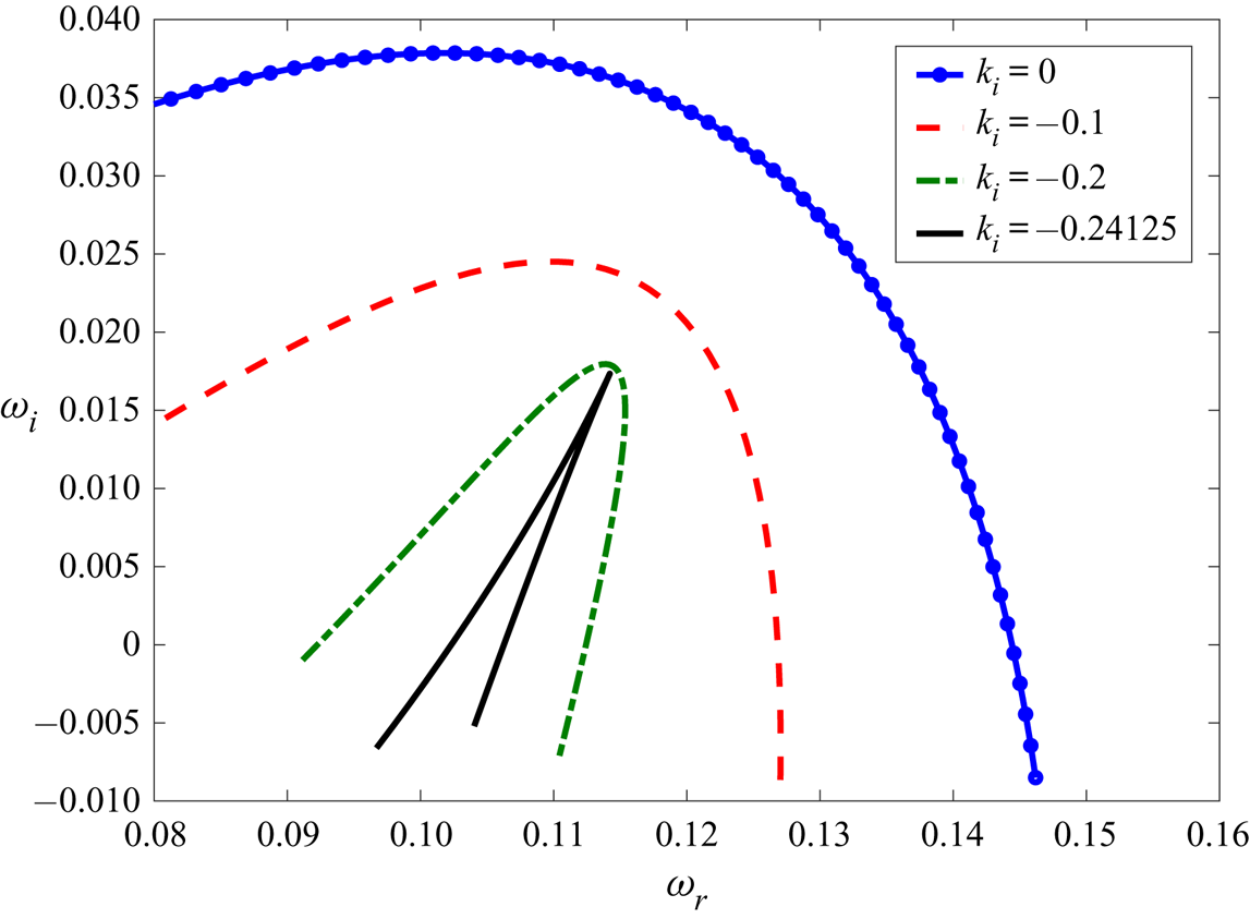
Figure 10. The formation of the genuine cusp point,  $\omega _0=0.1142+0.01734i$ in the $\omega$-plane at $a=10^{-4},b=2,\mu _r=0.1,V_r=0,\varGamma =10^{-3}, \varSigma _1=1$ and $\varSigma _2=1$. A straight line parallel to $\omega _i$ axis, drawn from the origin of the cusp point intersects the temporal stability curve ( $k_i=0$) once, thus the formed cusp point is genuine. Since the cusp point is genuine and possesses $\omega _i>0$, the flow is absolutely unstable.
According to the method of Kupfer et al. (Reference Kupfer, Bers and Ram1987), a cusp point in the  $\omega$-plane must correspond to a saddle point in the $k$-plane. To obtain the saddle point in the $k$-plane, a matrix of $\omega _r$ and $\omega _i$ values is generated by varying both $k_r$ and $k_i$ and (using MATLAB built-in functions) isocontours are obtained as shown in figure 11. The cusp point ( $\omega _0$) of figure 10 and saddle point ( $k_0$) of figure 11 represent a local mapping of the type $\omega -\omega _0 \sim (k-k_0)^2$, which shows that the saddle point in the $k$-plane is of first order.
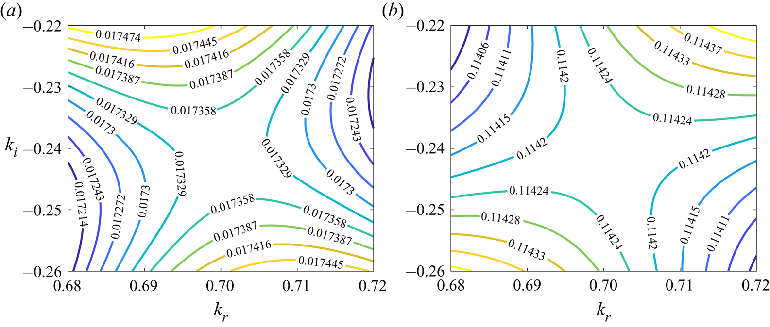
Figure 11. The existence of the first-order saddle point,  $k_0=0.7010 - 0.24125i$ in the $k$-plane corresponding to the cusp point shown in figure 10. The parameters are, $a=10^{-4},b=2,\mu _r=0.1,V_r=0,\varGamma =10^{-3}, \varSigma _1=1$ and $\varSigma _2=1$. Panels (a) and (b) show iso-contours for $\omega _i$ and $\omega _r$, respectively. The figure shows the presence of the first-order saddle point in the present model.
Computation of the cusp point is a time-consuming procedure since an analytical form of the dispersion relation is not available. Thus, unlike for the temporal stability analysis, critical parameters are not determined. Instead, parameters are varied in figures 12 and 13(a) with respect to those used to obtain figure 10 and the corresponding variation in  $\omega _{i0}$ is noted and then used in determining the stabilising or destabilising role of the parameters. In figure 12(a), $\varGamma$ is decreased with respect to figure 10 and leads to the absence of the absolute instability, implying a stabilising effect of decreasing $\varGamma$. This also shows that for the existence of the absolute instability, similar to the temporal instability, there exists a critical value of $\varGamma$ at which the flow undergoes a transition from a convectively unstable to an absolutely unstable state. Figure 12(b) shows the effect of varying the dimensionless thickness of the DS, where increasing $a$ by two orders of magnitude compared to figure 10 leads to the disappearance of the absolute instability. This also shows that even when the temporal analysis exhibited an unconditionally unstable region at low $a$, it is absent for the absolute instability.

Figure 12. The effect of variations in (a) the scaled plate velocity,  $\varGamma$; (b) scaled DS thickness, $a$; (c) scaled thickness of fluid $2$,
$2$,  $b$; and (d) viscosity ratio, $\mu _r$, on the absolute instability at $\varSigma _1=\varSigma _2=1$. All figures in the panels are obtained by varying one parameter with respect to the parameters used in obtaining figure 10. In (a), the cusp point at $\omega _0=0.2762-0.07595i$ shows the stabilising effect of increasing $\varGamma$. Thus, unlike temporal instability, at low $a$, the unconditionally absolute instability does not exist. Panel (b) shows the cusp point formation at $\omega _0=0.2763-0.07583i$, stabilising effect of increasing $a$. The cusp point forms at $\omega _0=0.11699 + 0.00592i$ in (c) for lower $b$ compared to figure 12(d) – a stabilising effect of decreasing $b$ due decreased $\omega _{i0}$. Panel (d) illustrates the stabilising effect of increasing $\mu _r$, as it increases from $0.1$ to $0.5$, the cusp point shifts from $\omega _0=0.1142+0.01734i$ to $\omega _0=0.12982 - 0.004889i$. (a) $a=10^{-4},b=2,\mu _r=0.1,V_r=0,\varGamma =10^{-5}$; (b) $a=10^{-2}, b=2,\mu _r=0.1,V_r=0,\varGamma =10^{-3}$; (c) $a=10^{-4},b=1,\mu _r=0.1,V_r=0,\varGamma =10^{-3}$ and (d) $a=10^{-4},b=2,\mu _r=0.5,V_r=0,\varGamma =10^{-3}$.

Figure 13. Panel (a) shows the formation of the cusp point at  $\omega _0=0.106659 + 0.019357i$ for the counter-flow configuration. Comparing with figure 10, the present figure shows that counter-flow is less stable. Panel (b) illustrates the existence of absolute instability even for $a>1$, albeit at higher $\varGamma$. The cusp point formation occurs at $\omega _0=0.19957 + 0.0037453i$. The other parameters used in these calculations are $b=2,\mu _r=0.1,\varSigma _1=1$ and $\varSigma _2=1$. (a) $a=10^{-4},V_r=-1,\varGamma =10^{-3}$ and (b) $a=3,V_r=0,\varGamma =0.9$.
In figure 12(c), compared to figure 10,  $b$ is decreased from $b=2$ to $b=1$, resulting in a decreased growth rate of the absolute instability ( $\omega _{i0}$) by one order of magnitude, demonstrating the strong stabilising effect of decreasing $b$. The effect of varying $\mu _r$ on the instability is illustrated in figure 12(d), where $\mu _r$ is increased from $\mu _r=0.1$ (figure 10) to $\mu _r=0.5$. As seen with the temporal instability, increasing $\mu _r$ has a stabilising effect on the absolute instability.
Lastly, figure 13(a) shows that the counter-flow configuration is favourable for inducing the absolute instability, illustrated by the fact that  $\omega _{i0}$ is higher for $V_r=-1$ than $V_r=0$ (figure 10). The absolutely unstable flow implies that the disturbances must spatio-temporally grow both in the downstream and upstream directions. We suspect that the counter-flow configuration is more easily amenable to the spatio-temporal growth of the disturbances in the upstream direction since fluid 2 is exerting a shear stress on the DS in the upstream direction due to the flow in negative $x$-direction. Such a shear stress can then help amplify the disturbances in the negative $x$-direction. Furthermore, fluid 2 can also convect the disturbances in the negative $x$-direction under the counterflow configuration, which is essential for the spatial convection of the disturbances. These could be the reasons that the counterflow is more prone to an absolute instability.
The preceding results are concerned with the existence of the absolute instability at low  $a$. However, the absolute instability also exists at higher $a$, provided that $\varGamma$ is also sufficiently high, as shown in figure 13(b). To conclude, by carefully adjusting the properties of the fluids and the DS, it is possible to introduce absolute instability in the system, which can in turn be used potentially to enhance mixing.
The parametric regime to observe the absolute instability in the experiments can be obtained as follows. From figure 10, the absolute instability exists for the parameters  $a=10^{-4},b=2,\mu _r=0.1,V_r=0,\varGamma =10^{-3}, \varSigma _1=1$ and $\varSigma _2=1$ which corresponds to $V_1 \sim 10^{-1}-10^{-3}\ \textrm {m}\ \textrm {s}^{-1}$, for a membrane of shear modulus $G \sim 10^{5} \ {{\rm Pa}}$ and channel height $R \sim 10^{-4} - 10^{-6}\ \textrm {m}$ which is achievable in the practical applications. Furthermore, from figure 10 and 11, the spatial and temporal growth rates of the absolute instability at the above parameters are $\omega _i=0.01734$ and $k_i=0.24125$, which seem detectable, experimentally. Using $k_r$ value from figure 11, the minimum length of the DS necessary to observe the above instability is of $O(1)\ \textrm {m}$.
4. Conclusions
The present study examined the linear temporal and spatio-temporal stability of simple shear flows coupled by an elastic, deformable solid layer. The fluids are Newtonian while the DS is described using linear elasticity. Such a fluid–DS–fluid coupling can be encountered in microfluidics, membrane separation and formation as well as in physiological systems such as cells and the heart. The present study illustrates the effect of the coupling between the fluids, as mediated by a finite-thickness DS, on the elastohydrodynamic instability and the existence of absolute instability.
At a sufficiently high dimensionless thickness of the DS ( $a$), a viscous instability is predicted – in agreement with the plane Couette flow past a plate lined by a DS. Under these conditions, the two flows on either side of the DS are hydrodynamically decoupled. However, at low $a$, the flows interact via the DS, which affects the viscous mode of the instability. The predicted instability arises from the energy exchange between the fluids and the DS via the tangential velocities at the interface. The interaction lowers the value of $\varGamma _c$ ( $\varGamma$ represents the shearing motion) required to destabilise the finite wave disturbances, eventually leading to an unconditionally unstable region. The existence of the unconditionally unstable region strongly depends on the thickness and viscosity of fluid $2$, i.e. in dimensionless terms $b$ and $\mu _r$, respectively. While this unstable region is present at low $\varGamma$ and $k$ (the wavenumber), it is accompanied by a very small growth rate of the perturbations. Such a low value of $\varGamma$ and practical restrictions on $k$ define a parametric limit within which the predicted instabilities may be observed in experiments and applications.
To further understand the role of the DS in triggering and controlling potential mixing in practical applications, a spatio-temporal stability analysis was carried out. The analysis revealed the existence of the absolute instability in the present system, however, at much higher  $\varGamma$ compared to that required for triggering the temporal instability. At low $a$, since the growth rate of the disturbances is small, the existence of the absolute instability can be highly useful since it will enhance mixing. Finally, in practical applications, the DS can be of a length comparable to the widths of the fluids. In such cases, a full global stability analysis is required and may give rise to new types of instabilities, presenting a possible next step in understanding the effect of the fluid–fluid coupling via a deformable solid on elastohydrodynamic instabilities.
Acknowledgements
This research was partially supported by grants 2018/17 and 356/18 from the Israel Science Foundation (ISF). R.P. was partially supported by the Technion Funds Postdoctoral Fellowship. We thank the anonymous reviewers for their careful reading of the manuscript and their many insightful comments and suggestions which helped in improving the manuscript.
Declaration of interests
The authors report no conflict of interest.


 Open access