


Introduction
The Southern Patagonia Icefield (SPI, Fig. 1) is a temperate ice mass (Warren and Sugden, Reference Warren and Sugden1993) that spans the territories of Southern Chile and Argentina, and constitutes most of the land ice stored in South America (Pfeffer and others, Reference Pfeffer2014). This region has become increasingly important due to its global sea level rise contribution (Rignot and others, Reference Rignot, Rivera and Casassa2003; Willis and others, Reference Willis, Melkonian, Pritchard and Rivera2012b; Gardner and others, Reference Gardner2013). Most of the ablation zones of the SPI glaciers are retreating with high thinning rates, resulting in lake/fjord expansions, the growth in the number of proglacial lakes, the increasing occurrence of glacial lake outburst floods, massive calving events and landslides in formerly ice-covered areas (Wilson and others, Reference Wilson, Carrión and Rivera2016, Reference Wilson2018; Harrison and others, Reference Harrison2018; Lenzano and others, Reference Lenzano2018). These trends have been related to tropospheric warming (Rasmussen and others, Reference Rasmussen, Conway and Raymond2007) and precipitation changes (Carrasco and others, Reference Carrasco, Osorio and Casassa2008), although climate and ice melt models applied to the area have shown positive mass balances with an increasing trend between 1975 and 2011 (Schaefer and others, Reference Schaefer, Machguth, Falvey, Casassa and Rignot2015).
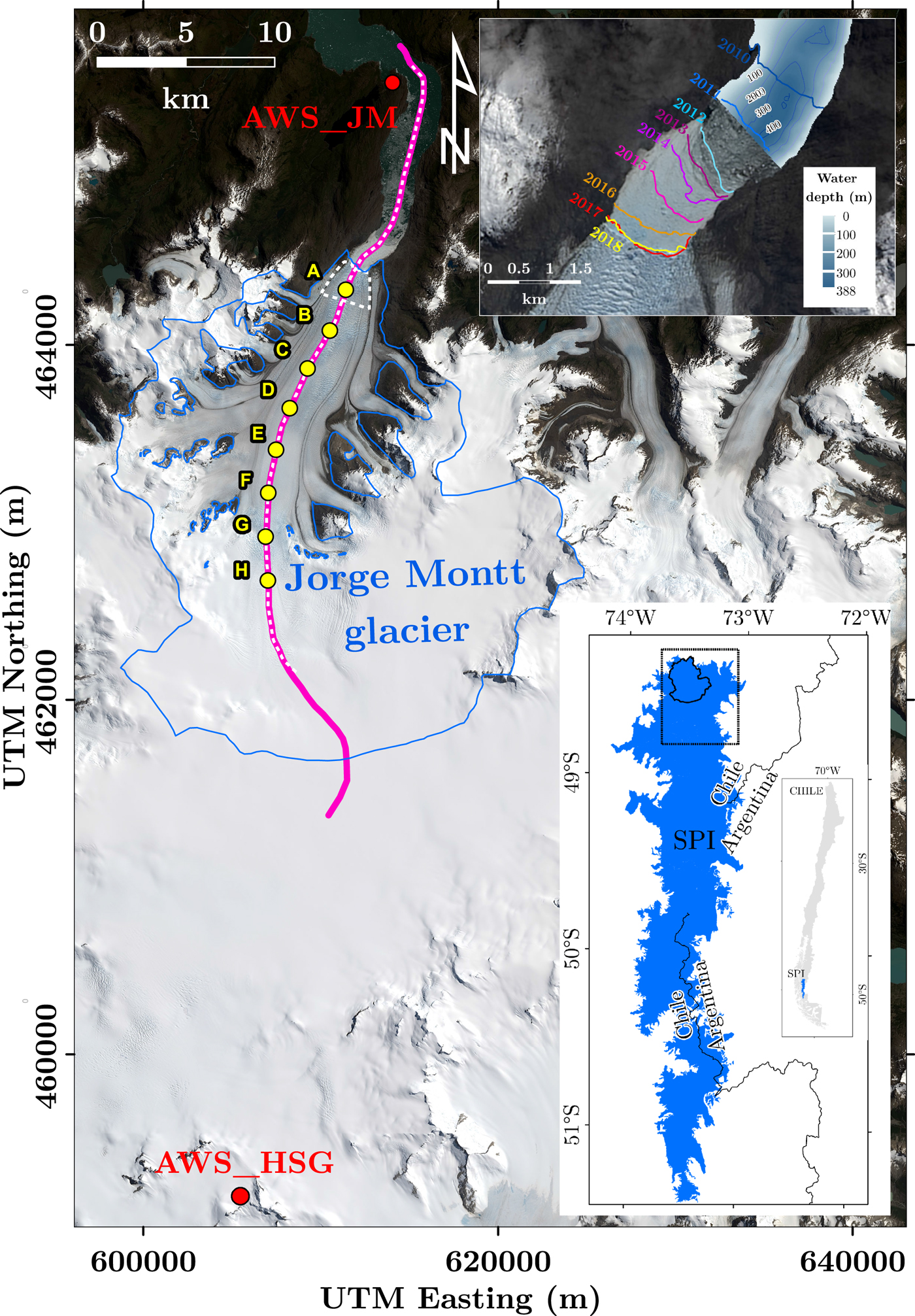
Fig. 1. Delineation of the SPI showing location of study area on the main map. Map of the study area (coordinates in UTM18S, WGS84) includes the glacier outline in 2015 and the calving front area in dashed white outline. Also shown the ice velocity profile overlapping the topographic profile discussed in the text (purple line), AWS sites (red dots), sampling points for velocity surface melt correlation (A–H). The inset shows frontal variations in 2010–2018 and water depth based on Rivera and others (Reference Rivera, Koppes, Bravo and Aravena2012b) and Moffat (Reference Moffat2014). Background images: Pansharpen Landsat OLI from 21 January 2015 (location map) and 14 February 2018 (inset).
Because most of the SPI glaciers are calving into fjords or lakes, the trigger for ice retreat has alternatively been attributed to ice dynamics (Mouginot and Rignot, Reference Mouginot and Rignot2015), characterised by ice speed acceleration, longitudinal stretching and ice thinning towards the glacier front, where deep fjords can provide the conditions for the ice to be buoyant. On the other hand, SPI glaciers typically comprise temperate ice (Warren and Sugden, Reference Warren and Sugden1993), therefore, when their fast flow tongues approach floatation, their fronts undergo widespread crevassing that is enhanced by the presence of abundant surface meltwater, resulting in rapid terminus disintegration. Under these conditions, the ice front is rarely afloat as a consequence of frequent calving, a process that ultimately controls glacier front changes.
Despite a number of recent studies focussing on frontal, area, velocity and elevation changes (Sakakibara and Sugiyama, Reference Sakakibara and Sugiyama2014; Foresta and others, Reference Foresta2018; Malz and others, Reference Malz2018), the characteristics of the ice–ocean interface that are thought to modulate retreat rates (including ice thickness near the glacier fronts, subaqueous melt and calving fluxes) are still poorly known in this region. This paper addresses some of these deficiencies, presenting new data from Jorge Montt tidewater glacier (48°S/73°W, Fig. 1) where ice dynamics has not previously been comprehensively studied. The glacier discharges into a proglacial fjord that is connected to the Pacific Ocean through the Baker channel (Moffat and others, Reference Moffat2018).
There is a long record of Jorge Montt Glacier changes; from a first map dated in 1898, coinciding with the Little Ice Age maximum position (Rivera and others, Reference Rivera, Koppes, Bravo and Aravena2012b), and extending through the second half of the 20th century. These changes have been researched by means of aerial photography, cartography and remote sensing, which have provided increasingly frequent and high-quality scenes in recent years. In this long-term record, three distinct periods of frontal changes have been described: the glacier retreated at a relatively low pace of 140 m a −1 as an average rate between 1898 and 1945, then it maintained a relatively stagnant frontal position between 1945 and 1975 with an average terminus retreat of 23 m a−1; thereafter, the glacier has been continuously retreating, with the strongest retreat period observed in the 1990s, with a total annual rate of 340 m a −1 between 1975 and 2018. The enhanced retreat cycles of Jorge Montt during historical times were greatly affected by water depth (Rivera and others, Reference Rivera, Koppes, Bravo and Aravena2012b). Submarine melt together with subglacial discharge, as well as wind forcing, are also thought to play a significant role in the fjord water properties and circulation (Moffat, Reference Moffat2014; Moffat and others, Reference Moffat2018).
This paper analyses the behaviour of tidewater Jorge Montt Glacier during recent decades with emphasis on its calving activity changes. The main aim is to compare these results with a glacier mass-balance model to determine the main factors explaining recent glacier responses.
Methods
Recent retreat and mass balance of Jorge Mott were assessed with combination of remote sensing and field observation methods: satellite and airborne imagery was used to calculate optical flow and frontal position changes, gravimetric and echosounding data enabled estimation of current and historic ice thickness and water depth, surface mass balance was computed with a simple temperature index model and, finally, calving rate and all relevant mass fluxes were calculated in the respective periods.
Satellite imagery and airborne glacier remote sensing
We processed and visually analysed a satellite dataset of Landsat (TM, ETM and OLI), ASTER and Sentinel optical images since 1986 (Table 1). In this procedure, we mapped the glacier outlines by manual digitisation of the ice fronts on co-registered images; then frontal change rates were determined by comparing each date position at the central ice flowline. Cross-correlation techniques were applied with available panchromatic (or best resolution) bands by using the COSI-CORR software package (Leprince and others, Reference Leprince, Barbot, Ayoub and Avouac2007). This method allowed us to calculate ice velocities between scenes of different dates by measuring relative displacement of surface features. We ran the feature tracking using the best visual quality and most closely timed scenes (in general weekly to fortnightly) on spatial resolutions not lower than the pixel size of Landsat 5 imagery (30 m). Only image pairs with correlation coefficients of ≥70% were preserved for the analysis. The calculated velocities were complemented with the freely available Global Land Ice Velocity Extraction from Landsat 8 (GoLIVE) dataset (Fahnestock and others, Reference Fahnestock2016; Scambos and others, Reference Scambos, Fahnestock, Moon, Gardner and Klinger2016). In comparison with the optical imagery spanning the period 1986–2018 (Table 1), the GoLIVE dataset has a lower spatial resolution (300 m) but more frequent sampling (every 16 days). We used velocity grids covering the period from 1 May 2013 to 30 April 2017. In addition, our results were compared with those obtained for 1986–2011 with feature tracking techniques by Sakakibara and Sugiyama (Reference Sakakibara and Sugiyama2014).

a Source: Land Processes Distributed Active Archive Center.
b Source: United States Geological Survey.
c Source: European Space Agency.
d Source: German Aerospace Center.
e Location in Fig 1.
We used several archive sources of the ice elevation records (Table 1): Chile's Instituto Geográfico Militar (IGM) regular cartography based on the aerial photography survey of SPI done in 1975, Shuttle Radar Topography Mission (SRTM) data from year 2000, several ASTER products obtained since 2003 and TanDEM-X data acquired by the German Aerospace Center (DLR) during 2011–2016.
Fjord bathymetry
Oceanographic cruises carried out by Centro de Estudios Científicos (CECs), the University of Concepción (Chile), the University of Washington (USA) and the University of British Columbia (Canada) have surveyed the fjord development following the glacier retreat since 1898. Water depths and bed characteristics were measured along longitudinal and transverse profiles (Table 1 and Fig. 1). We used echo-sounding and a Datasonics Bubble Pulser sub-bottom profiler acoustics system which allowed the penetration of up to 250 m of soft sediment deposits (Rivera and others, Reference Rivera, Koppes, Bravo and Aravena2012b). These measurements were extended in 2013 to within a few hundred metres from the glacier front position because ice melange precluded a closer approach to the ice front (Moffat, Reference Moffat2014). Upstream the present glacier front position the subglacial topography was mapped by a combination of radar and aerial gravimetry data collected in recent years (Millan and others, Reference Millan2019).
Frontal ablation and calving rate
We calculated the frontal ablation and calving rates of Jorge Montt Glacier for different epochs covering the period 1986–2018. We used optical satellite imagery separated by short-term periods to obtain ice velocities and a long-term frontal change record, along with various elevation datasets (Table 1) and measurements of ice thickness (Gourlet and others, Reference Gourlet, Rignot, Rivera and Casassa2016) and fjord bathymetry (Rivera and others, Reference Rivera, Koppes, Bravo and Aravena2012b) that enabled calculation of a corresponding ice flux.
At San Rafael Glacier (Northern Patagonia Icefield) modelling results show that basal sliding accounts for 98% of the observed surface ice velocity in the fast-flowing part of the glacier (Collao-Barrios and others, Reference Collao-Barrios2018). Following these results, we assume that on Jorge Montt Glacier the vertically averaged ice velocity $\bar {u}_{\rm i}$ equals the measured surface ice velocity v i (Pfeffer, Reference Pfeffer2007). The ice discharge Q i through a fluxgate is calculated by integrating ice velocity $\bar {u}_{\rm i}$
 across a transverse profile:

where L is the length of the transverse profile, H(x) is ice thickness at glacier width x and is calculated as a difference between surface elevation at, or closest to, a given epoch (IGM, SRTM, ASTGTM) and AIRGrav bedrock elevation (Table 1). The feature tracking algorithm mostly failed to provide reliable results near the ice front, therefore to provide a coherent dataset of ice flow velocity, we used a flux gate located 2 km up-glacier from a respective frontal position for ice flux calculations. Subsequently, assuming constant flux/mass-conservation along the flow, we calculate mean ice velocity at the front $\bar {u}_{\rm f}$ :
:

where A f is the cross-sectional area at the glacier front with ice thickness H = h + H w, h is ice height above water and H w is water depth. Subaerial calving rate $\bar {u}_{\rm c}$ is then calculated as a difference between mean ice velocity at the front and frontal change rate ∂l/∂t:

Finally, assuming that on longer timescales submarine frontal ablation follows subaerial calving rate, i.e. frontal ablation rate and calving rate are equal, frontal ablation flux Q f is calculated as a product of mean calving rate and cross-sectional area at the front:

In this approach, submarine melt is assumed to follow subaerial calving and, therefore, is integrated in the resulting frontal ablation volume, thus its partial contribution cannot be determined. As argued before, ice velocity, calving rate and frontal ablation are assumed to be constant along the vertical profile.
We also analysed some characteristics of calving along the glacier by applying a calving rate parameterisation based on water depth H w and calving front height h (Mercenier and others, Reference Mercenier, Lüthi and Vieli2018) using bathymetry and gravimetry data:

where $\tilde {B}=65\, {\rm MPa}\,^{-r}\, {\rm a}^{-1}$ is effective damage rate, ω = H w/H is relative water level, σth = 0.17 MPa is a damage threshold stress and r = 0.43 is a damage law exponent. This approach has a solid theoretic foundation that is based on detailed stress analysis and was calibrated on a set of Arctic tidewater glaciers (Mercenier and others, Reference Mercenier, Lüthi and Vieli2018). Therefore, it can be considered as a model that can explain or assess the importance of purely geometric drivers on calving rates. In our case, the subaerial ice cliff height h is assumed a constant 60 ±10 m. Water level height H w is determined by bedrock topography as measured by the bathymetric (Rivera and others, Reference Rivera, Koppes, Bravo and Aravena2012b) and gravimetric (Gourlet and others, Reference Gourlet, Rignot, Rivera and Casassa2016) surveys.
Meteorological data
Meteorological data were collected using two automatic weather stations (AWS). One AWS was located on a rock outcrop near to Jorge Montt Glacier front (48°15′13″S/73°27′36″W/193 m a.s.l., hereafter AWSJM, Table 1, Fig. 1) and measured air temperature (sensor Young 41382VC) and precipitation (Young 52202 rain gauge) with 1 hour temporal resolution between June 2014 and February 2018. The second AWS (hereafter AWSHSG, Table 1, Fig. 1) was located further south (48°49′55″S/73°34′53″W/1428 m a.s.l.), on a nunatak of Greve glacier. This station provides a continuous air temperature record between April 2015 and January 2017. We used gridded NCEP-NCAR reanalysis data to extrapolate temperature series during years lacking AWS records. Furthermore, the air temperature lapse rate was calculated using a common observation period between measurements at both AWSJM and AWSHSG.
The record of total precipitation measured at AWSJM was complemented with NCEP-NCAR reanalysis data (Kalnay and others, Reference Kalnay1996) between 2012 and 2017, and extrapolated over the glacier surface. We used the same precipitation gradient of +5%/100 m that was used by Schaefer and others (Reference Schaefer, Machguth, Falvey, Casassa and Rignot2015), and a threshold temperature for rain and snow of 2°C, the same as Koppes and others (Reference Koppes, Conway, Rasmussen and Chernos2011). Daily NCEP-NCAR reanalysis and AWSJM precipitation records have a correlation coefficient of 0.62 during the common period (2015–2017). The annualised RMSE of 340 mm is obtained. Consequently, the uncertainty of the precipitation measurements is estimated at ~15%.
Surface mass-balance terms
We assumed a simple approach by which the mass accumulation is added through snowfall and that ablation is mainly constrained to surface melt (Cuffey and Paterson, Reference Cuffey and Paterson2010). Due to the temperate regime and high crevassing of the glacier (Warren and Sugden, Reference Warren and Sugden1993), both liquid precipitation and surface meltwater are assumed to be drained to the bed (Fountain and Walder, Reference Fountain and Walder1998) and subsequently discharged subglacially at the front, forming a buoyant plume (Moffat and others, Reference Moffat2018).
In the absence of solar radiation measurements over the glacier, we applied a simple degree-day model (DDM) relying on air temperature as a single input variable to calculate surface melt (Hock, Reference Hock2005; Wake and Marshall, Reference Wake and Marshall2015) using the closest AWS data. This method has been proven to be suitable in previous studies in the SPI (Takeuchi and others, Reference Takeuchi, Naruse and Skvarca1996; Stuefer, Reference Stuefer1999; De Angelis, Reference De Angelis2014). The DDM is calculated according to this formula:

where M is the snow and ice melt (mm w.e. °C−1 d−1) in a period n of time interval Δt (day), T + is the accumulated positive daily air temperatures (°C) and DDF is a degree-day factor.
DDF values for snow surfaces above the local equilibrium line altitude were fixed at 4.92 ± 1.54 mm w.e.°C−1d−1 while in the ablation zone the DDF was 7.17 ± 1.72 mm w.e. °C−1 d−1 based on Radić and Hock (Reference Radić and Hock2011). The assumption of these DDF values over the entire glacier constitutes the main source of surface melt uncertainty estimated in ~25% of net surface melt.
Results
Surface mass balance
The total specific precipitation for the whole glacier in 2012–2017 (rain+snow) ranges from a minimum of 2.45 ± 0.37 to a maximum 2.96 ± 0.44 m w.e. a−1. The snow fraction, hereafter accumulation, constitutes 70–80% of this total yearly received precipitation (Fig. 2), with a resulting range of 1.76 ± 0.26 to 2.39 ± 0.36 m w.e. a−1. The maximum specific values are ≈4.5 ± 0.68 m w.e. a−1 at the highest elevations around ~1800 m a.s.l. (see Suppl. Fig. S1) where rainfall is close to 0 m w.e. At the tidewater front, snowfall reaches between 0.1 and 1 m w.e. a−1 while rain reaches ≈2 m w.e. a −1. In 2016 particularly low values in snowfall were recorded over the glacier. Total snow accumulation varies between 0.79 ± 0.12 km3 w.e. a−1 in 2016 and 1.07 ± 0.16 km3 w.e. a−1 in 2017 (Table 2).
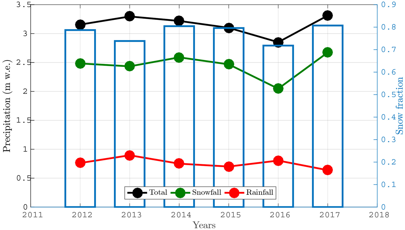
Fig. 2. Snow fraction of total precipitation at Jorge Montt Glacier between 2012 and 2017.
Table 2. Jorge Montt Glacier mass-balance components calculated for years 1986–2018 (km3 w.e. a−1)

AWSJM and AWSHSG air temperature records are statistically correlated (Fig. 3a). However, the temperature lapse rate shows significant interdaily variability in response to synoptic conditions and thermal inversion episodes. The location of AWSJM away from the ice–atmosphere interface is reflected with a milder weather and higher thermal amplitude, with mid-summer temperatures reaching nearly 15oC. Because the aim was to compute surface melt on a yearly basis, we used the average lapse rate of −0.0058°C m−1 (Fig. 3b). Since the NCEP-NCAR 1000 hPa pressure level air temperatures were highly correlated with the AWSJM air temperatures (Fig. 3c), we used this NCEP-NCAR dataset to reconstruct the missing period, yielding an average value of 6.97oC for the AWSJM air temperatures. The resulting 2012–2017 air temperature series, corrected by the cooling effect over the glacier boundary layer (Carturan and others, Reference Carturan, Cazorzi, Blasi and Dalla Fontana2015; Bravo and others, Reference Bravo2019b) assuming a 1oC reduction bias, is shown in Figure 3d. The distributed temperature model for the glacier shows a warmer area comprising the lower outlet tongue and a second area comprising the ice plateau where stronger winds and ice–atmosphere cooling feedbacks are evident (Fig. 3e). The highest surface melt rates are produced in the lowest-elevation glacier area; below 200 m a.s.l. (Fig. 4a), with values reaching 16–18 m w.e. a−1. Melt is nearly negligible at ~1300 m a.s.l. The distributed surface melt between 2012 and 2017 ranges from 1.43 ± 0.36 to 1.98 ± 0.50 km3 w.e. a−1 in 2016, with a mean value of 1.66 ± 0.41 km3 w.e. a−1 (Table 2, Fig. 4b).

Fig. 3. (a) Observed air temperatures at AWSJM and AWSHSG, (b) temperature lapse rate bounded by 75 and 25% quartiles, red horizontal line and filled circle depicts statistical median and mean, respectively, and crosses are outlier values, (c) mean daily temperature scattering between AWSJM and T1000 (NCEP-NCAR), orange line is the best-fit curve and dashed line is the one-to-one relation, (d) reconstructed AWSJM air temperatures and (e) distributed air temperatures in January 2012–February 2018 after cooling effect correction. Contour lines every 100 m in white, coordinates in UTM18S, WGS84.
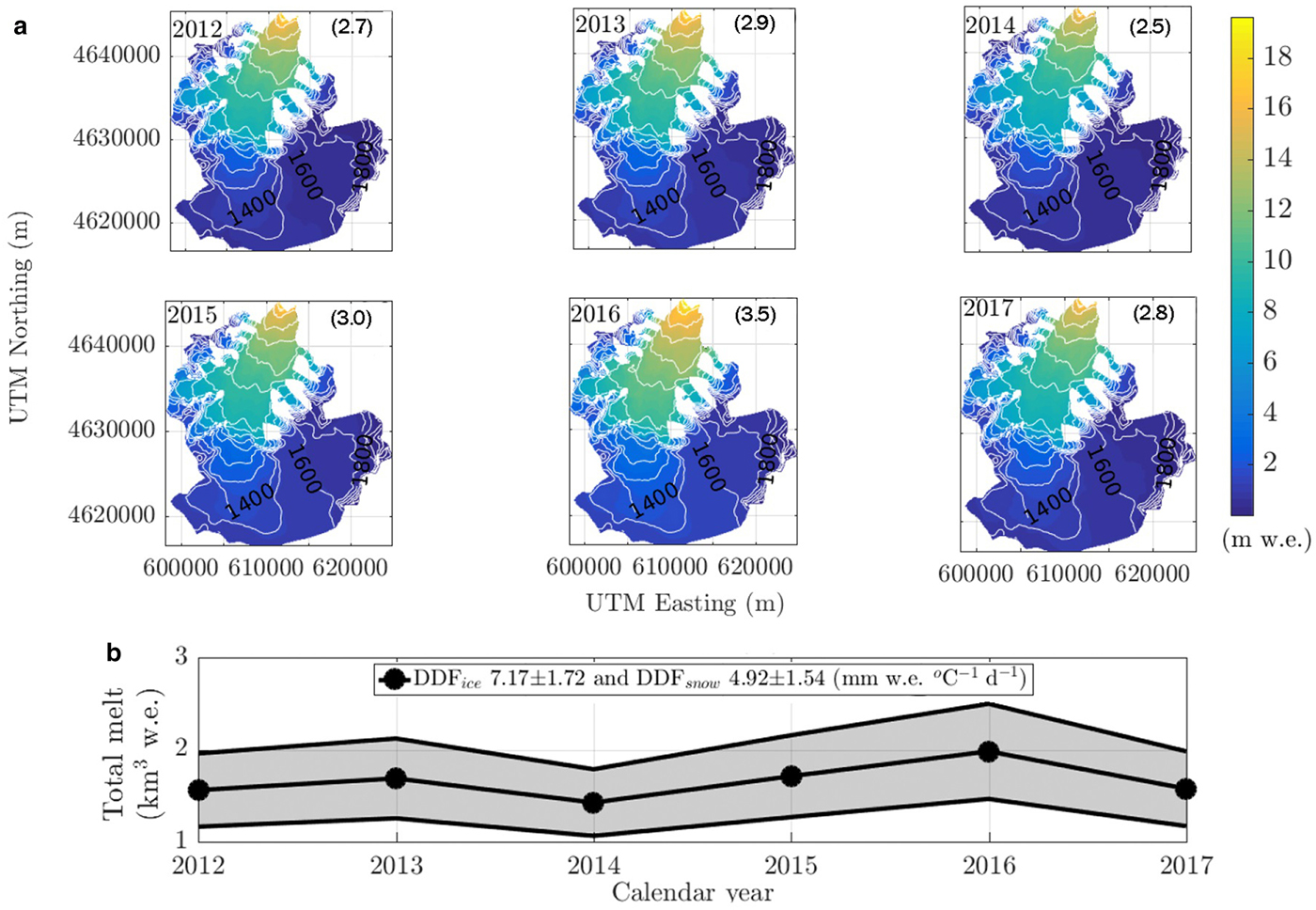
Fig. 4. (a) Distributed surface melt of Jorge Montt Glacier between 2012 and 2017. Annual mean values in m w.e. are shown in parentheses. Contour lines every 100 m in white. (b) Total surface melt in km3 w.e. Coordinates in UTM18S, WGS84.
Frontal variations
Between 2011 and 2018, the calving front of Jorge Montt Glacier retreated at rates between 640 and 200 m a −1 (Fig. 1), totalling a net change of −2.7 km. This implies that 5.2 km2 of ice area was lost in this 7-year period. The maximum retreat rate (640 ma −1) was observed in 2011–2012, when the fjord was covered by an ice melange and when an expansion of large crevasses in most of the calving front was observed. The retreat continued at lower rates between 2012 and 2014 (200 m a −1 in 2012–2013 and 323 m a −1 in 2013–2014) despite a large ice break-off event that impacted the calving front according to the satellite image acquired on 1 April 2014. Thereafter, the retreat increased to 560 m a −1 in 2014–2015 and 511 m a −1 in 2015–2016, when the glacier was highly crevassed down to the calving front. Subsequently, the retreat rate first decreased to 333 m a −1 in 2016–2017 before the ice front position fully stabilised between 2017 and 2018 (Fig. 1).
Surface ice velocity patterns
Over the entire glacier record, ice velocities increase from the accumulation zone where minimum values were ≈0.5 km a−1 towards the calving front and where maximum values reached ≈10 km a−1. The ice flow increases from the plateau into the outlet glacier (~28 km from 1986 ice front, Fig. 5). Therefore, extended crevasses surrounding the equilibrium line are observed in the optical satellite imagery (Fig. 1) as ice topography drops from 1300 m a.s.l. (Fig. 6) down to the lower tongue. There is a second zone of highly extensional flow in the terminal part of the glacier, where ice velocities reach maximum values. A strong increase in ice flow velocity was observed from 1986 to 1998 in the lowermost kilometres of the glacier, followed by relatively stable flow in 2002/03 and then again accelerating velocities in 2011 (Fig. 5). Simultaneously, the surface topography of the whole ablation zone (approximately below 1300 m) has been thinning at high rates, with annual values ranging from $-3 {\, {\rm m \,a}^{-1}}$ to −20 m a −1 at the calving front between 1975 and 2000, and thereafter from $-2 {\,\rm {m\,a}^{-1}}$
 to −21 m a −1 (Fig. 6).
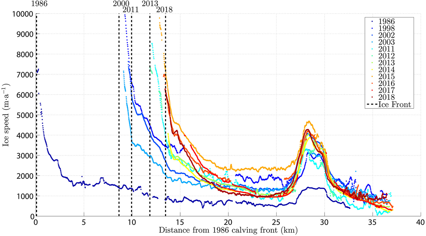
Fig. 5. Jorge Montt surface ice velocities along the central flowline (1986–2018) and frontal positions (dashed lines) based on Rivera and others (Reference Rivera, Koppes, Bravo and Aravena2012b) for 1986–2010 and this work for 2013–2018.
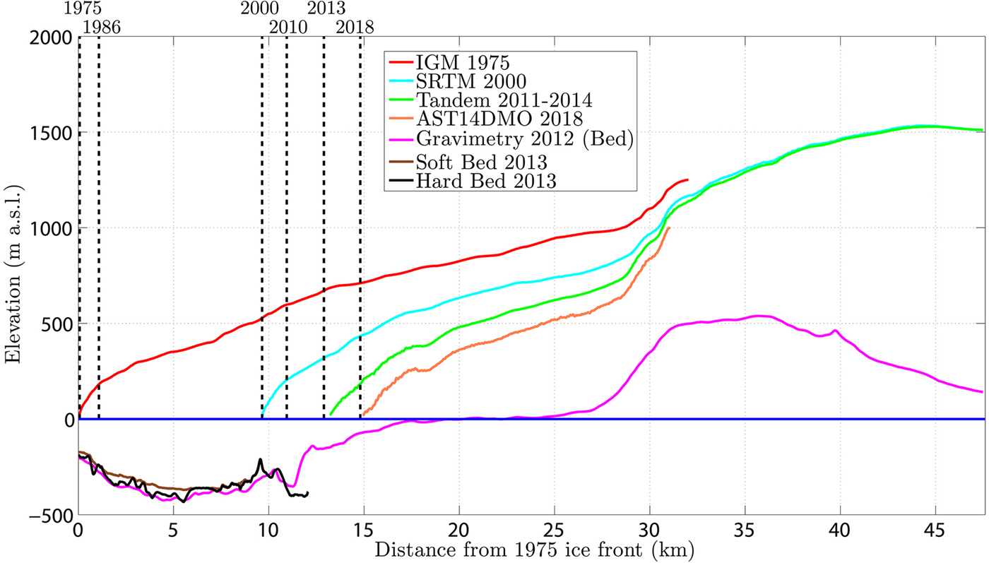
Fig. 6. The geometry of Jorge Montt Glacier in recent decades: ice elevation data from the 1975 Instituto Geográfico Militar official cartography (red), Shuttle Radar Topography Mission for 2000 (cyan), TanDEM Mission for 2011–2014 (green) and AST14DMO for 2018 (orange), ice bed from Gourlet and others (Reference Gourlet, Rignot, Rivera and Casassa2016) for 2012 (purple), ice front positions (dashed vertical lines) based on Rivera and others (Reference Rivera, Koppes, Bravo and Aravena2012b) for 1986–2010 and this work for 2013–2018. Soft bed (brown) is the bathymetry where sediments have been mapped and hard bed (black) refers to the bedrock underlying soft sediment deposits, both surveyed with a sub-bottom Bubble Pulser profiler in 2013.
In the majority of the datasets, the feature tracking algorithm failed to provide meaningful results in the area between the ice front and 0.5–1.0 km upstream, mainly due to extensive ice crevassing in this area and because near the terminus the ice flow is too fast compared with the repeat paths of the satellite imagery. Additionally, the velocity dataset in 2012 is very limited due to the presence of SLC-off gaps in Landsat 7 ETM+ imagery. The maximum ice velocity in 2013 and 2014 was around 4.0 km a−1 at a position 1–2 km upstream from the calving front. In turn, ice velocity in 2015 reached similar maximum values to those of 1998 (~10 km a−1) in close proximity to the calving front (Fig. 5). This coincides with a stronger frontal retreat observed in that period. Afterwards, the maximum ice velocities were lower and reached 7.0 km a−1 in 2016 and 3.5 km a−1 in 2017 (Fig. 5).
An example of the ice velocity field for the tidewater calving front area (60–200 m a.s.l., see location in Fig. 1) of Jorge Montt Glacier is shown in Figure 7. There is a marked increase towards the main flowline area from ice margins, comprising both lateral moraines. The part of the glacier that directly reaches the fjord has extremely high velocity values, up to 10–11 km a−1.
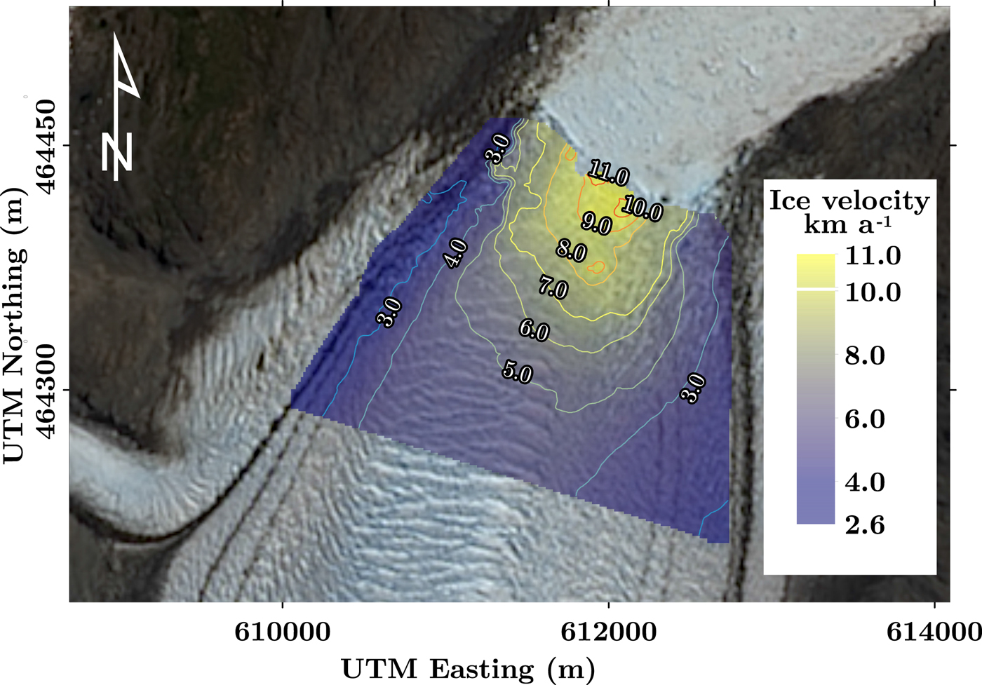
Fig. 7. Ice velocities in the terminal part of Jorge Montt Glacier in the period 14–21 January 2015. Background: Pansharpen Landsat OLI scene from 21 January 2015, coordinates in UTM18S, WGS84. Bi-spline interpolation applied.
Frontal ablation
There is a strong increase in frontal ablation from 1986 to 1998, following ice acceleration, when the glacier was retreating rapidly into deep waters (Rivera and others, Reference Rivera, Koppes, Bravo and Aravena2012b). Estimated average ice velocities Eqn (2) together with the subaerial calving rate Eqn (3) yielded a frontal ablation flux Eqn (4) of 4.74 ± 1.21 km3 w.e. a−1 (Table 2) in 1998, versus the 2.99 ± 0.36 km3 w.e. a−1 in the same year based on the parameterisation of Mercenier and others (Reference Mercenier, Lüthi and Vieli2018) (Fig. 8). High frontal ablation is observed again in 2011; thereafter there are oscillations, with the highest value in 2015 (Table 2) resulting from larger ice velocities in this latter period.
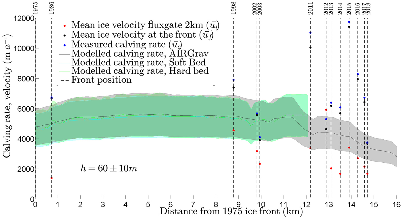
Fig. 8. Ice velocity and calving rate of Jorge Montt Glacier along a longitudinal profile during its retreat. Modelled calving rates were calculated with a relative water depth based parameterisation of Mercenier and others (Reference Mercenier, Lüthi and Vieli2018) using subaerial ice cliff height h set to 60 ± 10 m and three datasets for bedrock topography (gravimetric measurements, soft and hard bed bathymetry profiling). Soft bed (cyan) is highlighted above hard bed (green) where sediments are present. Note AIRGrav dataset was corrected by Gourlet and others (Reference Gourlet, Rignot, Rivera and Casassa2016) based on fjord bathymetry measurements presented in this work.
Mass-balance components partitioning and subglacial discharge
The total mass balance of Jorge Montt Glacier was consistently negative in years 2012–2017 (Fig. 9). This contrasts with results of Schaefer and others (Reference Schaefer, Machguth, Falvey, Casassa and Rignot2015) for 1975–2011 when the surface mass balance was calculated to be slightly positive. Surface melt was significantly lower than frontal ablation in 2015 when the former was 1.71 ± 0.43 km 3 w.e. a−1 and the latter reached 3.81 ± 1.10 km 3 w.e. a−1. In other years, both values were almost equal (ratio close to 1 in Fig. 9) within their respective error bounds. Subglacial discharge, calculated as a sum of surface melt and liquid precipitation, remained fairly stable throughout the 2012–2017 period while oscillating around 2 km3 w.e. a−1, reaching a maximum value of 2.29 ± 0.50 km3 w.e. a−1 in 2016 and a minimum of 1.84 ± 0.40 km3 w.e. a−1 in 2017. At the same period, frontal ablation flux was much more dynamic and resulted in a high variability of the frontal ablation to subglacial discharge ratio (Fig. 9).
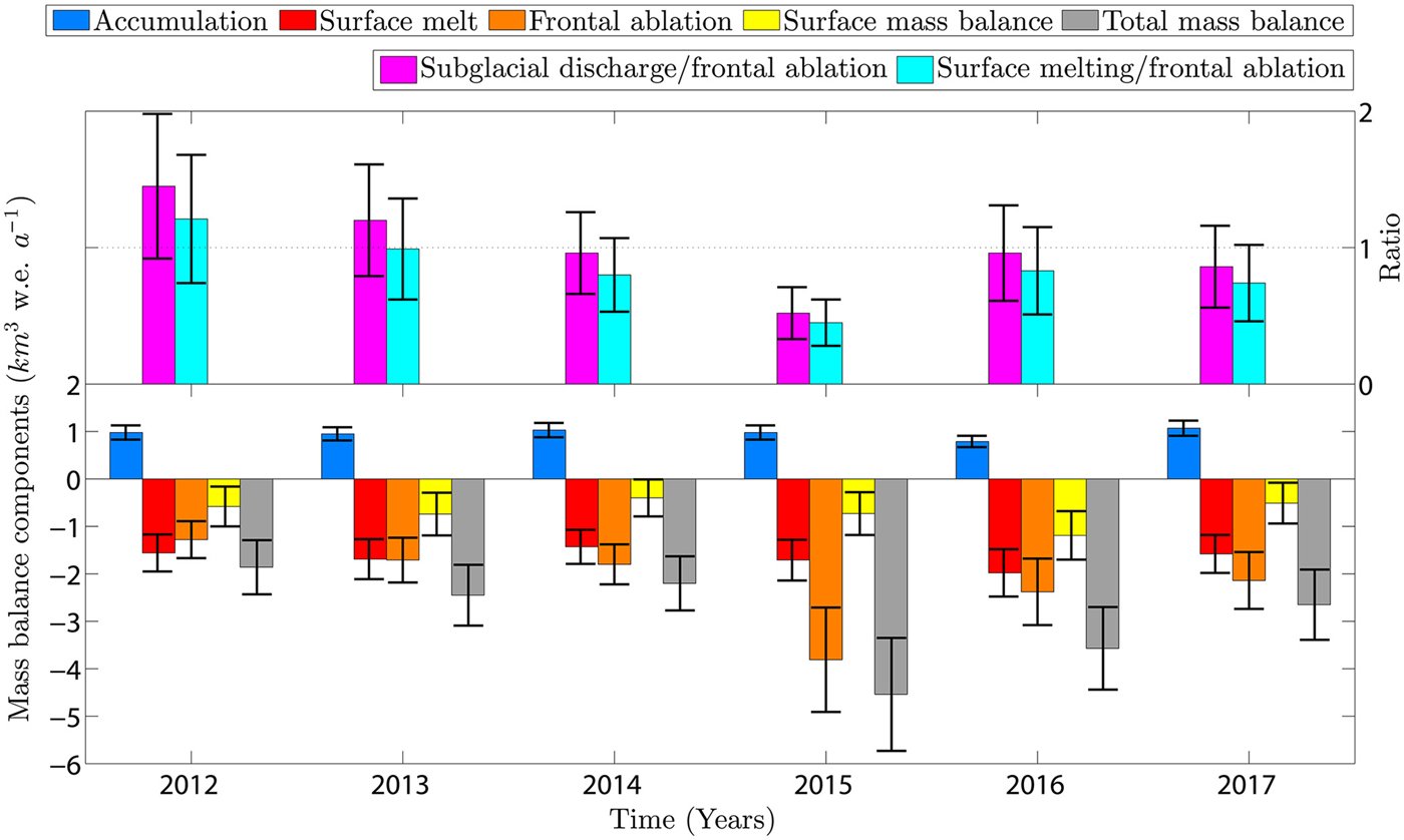
Fig. 9. Mass-balance components of Jorge Montt Glacier in 2012–2017: subglacial discharge to frontal ablation and surface mass balance to frontal ablation ratios in the top panel; accumulation, surface melt, frontal ablation, SMB and TMB in the bottom panel.
Discussion
In the period 2011–2018, Jorge Montt retreated 2.7 km (equivalent to an ice area loss of 5.2 km2), a process which can be interpreted to have started in 2010, when it was reported the glacier was calving into waters nearly 400 m deep (Rivera and others, Reference Rivera, Corripio, Bravo and Cisternas2012a). In this process, the calculated ice velocities were the highest values throughout the historical record as compared with datasets for the period 1986–2011, with the sole exception of the peak reached in 1998 (Rivera and others, Reference Rivera, Koppes, Bravo and Aravena2012b). The spatial pattern of ice velocity is consistent across different studies (Muto and Furuya, Reference Muto and Furuya2013; Sakakibara and Sugiyama, Reference Sakakibara and Sugiyama2014; Mouginot and Rignot, Reference Mouginot and Rignot2015) and is characterised by minimum velocities in the accumulation zone, ice flow velocity increasing downstream from the plateau into the outlet tongue (~1200 m a.s.l.) and strong re-acceleration near the calving front, which in our analysis reached a maximum of 10–11 km a−1 in 2015.
Upstream of the present ice front position ice thickness became progressively thinner and ~3 km from the present ice front, the glacier bed is above sea level (Fig. 6). As a consequence, the recent rates of ice retreat will continue to drive longitudinal stretching with strong ice thinning at least until the ice front stops calving when the glacier bed approaches sea level (Fig. 6).
These calculated ice velocities and frontal changes allowed determination of frontal ablation fluxes in recent decades. In 1998, the frontal ablation reached a maximum of 4.74 ± 1.21 km3 w.e. a−1, in an area where maximum water depth was higher than 300 m. In recent years, high frontal ablation, somewhat below 1998 value, were obtained with a maximum of 3.81 ± 1.10 km3 w.e. a−1 in 2015 and a minimum of 1.28 ± 0.39 km3 w.e. a−1.
These frontal changes and fluxes are accompanied by an overall negative mass balance. Total precipitation specific values between 2012 and 2017 range from 2.45 ± 0.37 to 2.96 ± 0.44 m w.e. a−1, which if neglecting the liquid phase (as rain percolates and is assumed to be subglacially discharged) drives mass accumulation ranging from 1.76 ± 0.26 to 2.39 ± 0.36 m w.e. a−1 (Table 2). In turn, the DDM based on common DDF values used in the SPI (Radić and Hock, Reference Radić and Hock2011) and corrections by cooling effects with nearest observations (0.8–1.2°C), accounts for overall surface melt in 2012–2017 (Table 2) with specific values between 3.19 ± 0.80 and 4.42 ± 1.10 m w.e. a−1. The severe drought recently recorded in Patagonia (Garreaud, Reference Garreaud2018) most likely played a role in explaining these negative surface mass balances, that ranged between −1.19 ± 0.51 and −0.40 ± 0.39 km3 w.e. a−1 (Table 2, Suppl. Fig. S2), or if averaged over the glacier area, between −2.65 ± 1.13 and −0.89 ± 0.87 m w.e. a−1. The mean value for 2012–2017 of −1.54 ± 0.98 m w.e. a−1 indicates a negative shift when compared with downscaling modelling that yielded 0.8 m w.e. a−1 surface mass balance between 1980 and 2010 (Schaefer and others, Reference Schaefer, Machguth, Falvey, Casassa and Rignot2015). By adding the frontal ablation, the total glacier mass balance of Jorge Montt ranges from −1.86 ± 0.57 to −4.54 ± 1.19 km3 w.e. a−1 (Table 2), or −10.12 ± 2.65 to −4.15 ± 1.27 m w.e. a−1. This highly negative total mass balance, consistent with the ice volume losses observed by the geodetic method (Rignot and others, Reference Rignot, Rivera and Casassa2003; Willis and others, Reference Willis, Melkonian, Pritchard and Ramage2012a; Abdel Jaber and others, Reference Jaber, Wael, Johnson and Rott2017; Willis and others, Reference Willis, Melkonian, Pritchard and Rivera2012b; Foresta and others, Reference Foresta2018), reveals a much larger importance of frontal ablation than previously thought. A simple comparison of our average of −6.41 m w.e. a−1 in 2012–2017 through surface mass balance and calving versus the −4.64 m w.e. a−1 in 2011–2017 solely by ice thinning (Foresta and others, Reference Foresta2018) supports this statement. Methodological issues including spatial resolution, timescales and ice density can also be argued to explain this discrepancy.
It is interesting to compare the frontal velocities and the calving flux of Jorge Montt with other Patagonian glaciers, for example with San Rafael, a tidewater glacier located in the western side of the Northern Patagonia Icefield (Rivera and others, Reference Rivera, Benham, Casassa, Bamber and Dowdeswell2007), that has been a focal point of interest due to its extremely high ice flow velocity. Here, velocity reached a maximum of 7.2 ± 0.4 km a−1, resulting in a calving flux in 2007 of 2.22 ± 0.05 km3 (Willis and others, Reference Willis, Melkonian, Pritchard and Ramage2012a). These very high numbers are smaller than the 11 ± 2 km a−1 maximum ice velocity measured at Jorge Montt front in 2015 and much smaller than the highest frontal ablation obtained in 1998 of 4.74 ± 1.21 km3. Other SPI lacustrine calving glaciers such as Ameghino (Stuefer, Reference Stuefer1999), Grey (Lliboutry, Reference Lliboutry1956) or Perito Moreno (Warren, Reference Warren1994) are characterised by much lower ice velocities and calving rates; even in case of the catastrophic retreat of Upsala Glacier in the 1990s its maximum calving velocity reached 1877 m a−1 (Skvarca and others, Reference Skvarca, De Angelis, Naruse, Warren and Aniya2002), which is almost an order of magnitude less than the maximum values of Jorge Montt. Our estimates place Jorge Montt among the fastest tidewater glaciers in the world.
This negative mass-balance trend took place while snow accumulation at Jorge Montt increased in the long term, between 1980 and 2015 (Bravo and others, Reference Bravo2019a), indicating that climate is not the main driving factor, and that instead, dynamic thinning is the primary control (Mouginot and Rignot, Reference Mouginot and Rignot2015). It is clear that this thinning must have been reinforced by surface processes however, such as a snow deficit as well as melt and meltwater percolation. We tested this relationship by analysing the correlation between surface melt and velocity, but the results were conclusive only in the lowest part of the glacier (Fig. 10), where high velocities were significantly related to surface melt. We found no correlation further upstream.
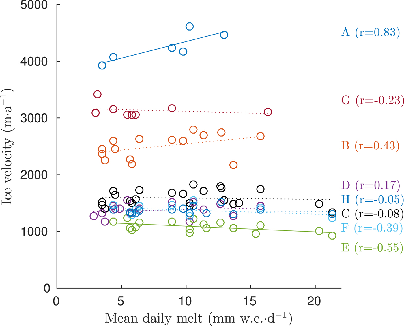
Fig. 10. GoLIVE surface ice velocities versus surface melt in 2013–2017 along profile A–H (see Fig. 1 for precise point location). Significant trends at 5% significance level are marked with continuous line (points A and E), and the insignificant trends are marked with a dotted line.
To explore the impact of fjord geometry on frontal ablation and retreat, we compared the modelled calving rates (Mercenier and others, Reference Mercenier, Lüthi and Vieli2018) with observed frontal ablation and retreat rates (Fig. 8). The model of Mercenier and others (Reference Mercenier, Lüthi and Vieli2018) is driven by the relative ice thickness only, disregarding other internal and external factors such as ice flow velocity, ice damage inherited from upglacier crevassing and thermal undercutting. Hence, in Jorge Montt Glacier it can explain the calving component related to the dynamic instability of the front approaching floatation. When observed frontal ablation rate diverges from the modelled value of calving rate we suggest that other factors, such as ice velocity fluctuation driven by a change in mass balance or thermal undercutting, are driving the retreat of the glacier front, which is otherwise at equilibrium at a particular water depth.
It is important to explore how the total mass-balance partitioning would follow if subglacial topography conditions change in the future. Assuming that subglacial discharge is equal to the sum of liquid precipitation and surface melt, i.e. that the entire rain and meltwater mass is routed through the englacial and subglacial drainage system and released at the front forming a buoyant plume and enhancing submarine melt, we use the ratio of frontal to surface ablation flux as a simple measure that describes the relative importance of these two main freshwater sinks: iceberg calving that mostly releases fresh water to the surface and shallow ocean layers (Enderlin and others, Reference Enderlin, Hamilton, Straneo and Sutherland2016; Moon and others, Reference Moon2018), and subglacial discharge, originating mostly from surface melt, that releases fresh water at the fjord bottom (Moffat and others, Reference Moffat2018). Here, the contribution of submarine melt as part of the frontal ablation flux is ignored. We are aware that this may be an oversimplification of the very complicated processes that are involved, but we argue that even with such a simple approach we can provide important clues about the possible future evolution of fjord hydrography. As a result, it appears that if Jorge Montt front retreats to shallow water as expected from AIRGrav bathymetry, most of the fresh water will be sourced from surface melt and will therefore be released subglacially at the front and will increase submarine melt rates. This is similar to modelling results of Amundson and Carroll (Reference Amundson and Carroll2018) that show a small lag between maxima of subglacial discharge and frontal ablation flux during retreat of a tidewater glacier. Simultaneously, iceberg production will diminish and less fresh water will be produced on the fjord surface as a spatially distributed source. Altogether, this might have important consequences on future fjord circulation (Moffat and others, Reference Moffat2018), sediment budget (Syvitski, Reference Syvitski1989) and nutrient fluxes (Bhatia and others, Reference Bhatia2013). As mentioned before, it is necessary to investigate how subglacial discharge will modulate the submarine melt. Modelling results of Moffat and others (Reference Moffat2018) show that the freshwater contribution from submarine melting at Jorge Montt during winter months equals the fresh water sourced from subglacial discharge. In our approach, submarine melting is not strictly separated from calving flux as they are considered in bulk as the frontal ablation flux. Nonetheless, modelled submarine melting rates of Moffat and others (Reference Moffat2018) are an order of magnitude lower than our reported calving rates, suggesting that the impact on the observed retreat is of secondary importance. Still, submarine melting can be an important trigger of calving through thermal undercutting (O'Leary and Christoffersen, Reference O'Leary and Christoffersen2013). Glacier and ocean modelling may provide a basis to sustain a hypothesis of glacier slow down and a switch into a retreat mode governed by surface slope, similar to observations at the Columbia Glacier (Venteris, Reference Venteris1999; O'Neel and others, Reference O'Neel, Pfeffer, Krimmel and Meier2005).
van der Veen (Reference van der Veen1996) explained the catastrophic retreat of Columbia Glacier as being driven by the dynamic thinning of the front due to an increase in ice flow velocities. In this case, relative depth at the terminus remained constant adapting to different water depth conditions during retreat. Therefore, the glacier remained close to flotation and calving was not determined by the absolute, but rather by the relative water depth. In such case, our assumption of bounds on h (60 ± 10 m) used in the calving rate parameterisation may not only serve as an error estimation, but also shows how calving rate will change when there is a small fluctuation of subaerial cliff height in response to water depth change during retreat. Moreover, wide bounds of plausible calving rates with varying h shown in Figure 8 reflect the ability of the calving front to adapt its calving rate through small changes in ice front geometry that can push the front towards conditions close to approach floating criterion as suggested for temperate glaciers by van der Veen (Reference van der Veen1996, Reference van der Veen2002). In this context, the temperate thermal structure of Jorge Montt Glacier not only allows for extremely high ice velocities, but also pushes the glacier towards a higher calving rate by its susceptibility to dynamic thinning at the terminus.
Maxima of the modelled calving rates do not exceed 7000 m a−1 and are significantly lower than the observed ones (Fig. 8). This difference becomes especially high in recent years (2013–2017) when, according to AIRGrav bathymetry estimates, the glacier front is supposed to have already retreated to a shallower bed (Fig. 6). Such discrepancy can be explained either by the simple structure and/or poor constraints in the model parameterisation of Mercenier and others (Reference Mercenier, Lüthi and Vieli2018), or by a possible underestimation of ice thickness in the region where AIRGrav survey has not been directly calibrated and validated with echosounding results (Gourlet and others, Reference Gourlet, Rignot, Rivera and Casassa2016). The results of Gourlet and others (Reference Gourlet, Rignot, Rivera and Casassa2016) have larger uncertainty in constrained, narrow valleys of the outlet glaciers such as Jorge Montt fjord which may have strong implications when ice dynamics is considered. Nonetheless, if the retreat continues into shallower bedrock it can be expected a future decrease in calving rate (Fig. 8) and consequently, a plausible deceleration of frontal retreat. This, however, will also depend on the future oceanic forcing that up to now remains poorly constrained.
Conclusions
We studied Jorge Montt tidewater glacier with multiple-source datasets including remote-sensing imagery and field data that were analysed together with a mass-balance model. The results suggest a dynamically driven response of the glacier characterised by sustained frontal retreat, high ice velocities and strong calving, altogether resulting in high mass imbalance during this decade. Jorge Montt calving rates obtained in this research are much higher than the rates observed in the other calving glaciers of the SPI. If the ongoing retreat continues, we estimate that the glacier will soon start to slow down, and approach a new and more stable condition due to the presence of bed topography above sea level ~3 km upstream from the present position.
Supplementary Materials
The supplementary material for this article can be found at https://doi.org/10.1017/jog.2019.47
Acknowledgments
This research was financed by CECs. CECs is a non-profit research organisation funded by the Basal Finance programme of CONICYT, among others. This paper also acknowledges FONDECYT grant #1171832. We thank the support of the Water Cadastre of Chile (DGA). Oceanographic data were collected by CECs and University of Concepción, Chile. We thank D. Sakakibara for providing Jorge Montt velocity profiles. C. Bravo acknowledges support from the CONICYT Becas-Chile PhD scholarship programme. C. Moffat and F. Bown acknowledge support from CONICYT-DRI Grant #2012-0012. Waters of Patagonia and the crew of ‘Don Tito’ provided valuable support in the field. We thank chief editor Hester Jiskoot, one anonymous reviewer and Jason Amundson for giving valuable comments and recommendations that greatly improved the quality of the article. We appreciate the editions to the manuscript and comments by Duncan Quincey.


 Open access