


NOMENCLATURE
- MPF(GW):
-
The distance traveled in miles per 1000 pounds of fuel burned when the aircraft gross weight has value GW
- GW:
-
Gross weight of aircraft
- EW:
-
Empty weight of aircraft
- w:
-
Freight load weight of aircraft
- g:
-
Fuel amount of aircraft
- R(g,w):
-
The range of aircraft with initial fuel is g and carrying freight weight w
- FC (g,w,d):
-
The fuel consumed by an aircraft flying a distance d, with initial fuel g, carrying freight weight w.
- FR (w,d):
-
The fuel required by a cargo aircraft to fly a distance d, carrying freight weight w;
1.0 INTRODUCTION
A problem or chaos occurring anywhere in the world can quickly become global in today’s risk and security environment. Therefore, countries with global interests should have the capability to move their military forces to anywhere around the world in a very short time and sustain their forces once deployed. Deployment refers to activities required to move military personnel and materials from a home installation to a specified destination. Although military deployment can be conducted by all available transportation modes, this study focuses on airlift operations.
Airlifting capability has been greatly improved since the Berlin Airlift, which ended the Berlin Blockade after World War II. During Operation Desert Storm in 1991, USAF C-130s moved nearly 14,000 personnel and 9,300 tons of cargo in ten days from King Fahd International Airport to Rafha with around 350 daily sorties(1). The USAF moved 18,539 personnel and 45,369 tons of cargo during Operation Joint Endeavor in December 1995 through February 1996(2).
Air refueling is the process of transferring fuel from one aircraft (the tanker) to another (the receiver) during flight, and plays a crucial role in airlift. During Operations Desert Shield and Desert Storm, approximately 400 tankers offloaded over 1.2 billion pounds of fuel to over 80,000 aircraft over 30,000 sorties, logging over 140,000 hours of flight time(Reference Barnes, Wiley, Moore and Ryer3). Operationally, air refueling extends the range of fighter and cargo aircraft and provides additional payload and loiter time for combat and combat support forces, allowing fighters and bombers to attack targets deeper in enemy territory and/or with greater payloads(Reference Camerer4).
Our research investigates whether air refueling can shorten the total time of an airlift operation and decrease the number of cargo aircraft sorties required in a deployment scenario where origin and destination are within the range of cargo aircraft. While air refueling is always a significant option for enabling aircraft to reach destinations beyond their unrefueled range, it is seldom used to support aircraft flights within range. However, by exchanging take-off fuel for additional cargo and then later refueling while airborne, it is possible to reduce the total number of cargo aircraft sorties needed to achieve a given air cargo movement requirement even within the cargo aircrafts’ range. The potential savings are limited by the cargo aircraft’s maximum takeoff weight limit, the distance between origin and destination, and available number of cargo and tanker aircraft.
Our paper proceeds as follows: Section 2 provides a review of the literature and discusses Yamani et al.(Reference Yamani, Hodgson and Martin–Vega5)’s model. We introduce our models in Section 3 and provide a numerical example in Section 4. We conclude in Section 5 with a discussion of the results and recommendations for further research.
2.0 BACKGROUND
While studies on airlift optimisation are abundant, research on the effects of air refueling on airlift is not so common. In this section, we provide a general overview of airlift operations literature from the air-refueling point of view and some examples of airlift optimisation studies.
Morton, et al.(Reference Morton, Rosenthal and Weng6) developed a multi-period, multi-commodity network optimisation model for strategic airlift assets. They aimed to minimise late deliveries while using demand satisfaction, aircraft balance, aircraft capacity, aircraft utilisation and aircraft handling capacity at bases as constraints in their model.
Baker et. al.(Reference Baker, Morton, Rosenthal and Williams7) used a large-scale linear programming model, called the NPS/RAND Mobility Optimiser (NRMO), for the optimisation of strategic airlift missions. Their model transports cargo and personnel within a given network using a fleet of aircraft, subject to some capacity and policy constraints. They provided two types of analyses. The first is the impact of enroute airfield capacity on the performance of airlift mission, and the second assesses the system’s ability under different fleet alternatives. NRMO provides better results (8% more daily cargo and 7% more personnel) than the Airlift Flow Module (AFM), which is the simulation model used by US Air Force Air Mobility Command.
Brigantic and Merrill(Reference Brigantic and Merrill8) described fundamental algebraic relationships that characterise the movement of cargo and passengers via strategic aircraft in an air mobility system. In particular, they presented formulae for computing the number of airlift missions required to deliver a given force a given distance; relationships for estimating the throughput or average number of tons per day that can be delivered to a particular airfield based on that airfield’s operating characteristics; and formulae for estimating the force total closure time based on airlift fleet parameters and the intended operational scenario. However, they did not include air refueling in their calculations.
Koepk et al.(Reference Koepke, Armacost, Barnhart and Kolitz9) took airports’ capacity constraint (called maximum on ground – MOG) for processing or parking into account, and extended Bertsimas and Stock’s(Reference Bertsimas and Stock10) integer program formulation for the Multi-Airport Ground-Holding Problem to the military air mobility problem. However, they used constant MOG values for each airport, even though MOGs are dynamic in real-life situations. They proposed an integer programming formulation that minimises the effects of overall disruptions according to aircraft mission priorities by enabling delays for certain aircraft on the ground.
Brown et al.(Reference Brown, Carlyle and Dell11) developed an integer linear programming model, the Air Tasking and Efficiency Model (ATEM), for the airlift operations in Iraq and Afghanistan. Their model creates routes for a heterogeneous aircraft fleet while optimising for maximum cargo transportation. Their model uses enroute landings for refueling rather than air refueling. They also proposed a heuristic for a quick solution.
Yuan and Mehrez(Reference Yuan and Mehrez12) studied air-refueling strategies for maximising the operational range of a heterogeneous aircraft fleet. They developed a heuristic optimisation model for finding an optimal air refueling chain. Their heuristic approach finds the average operational range within 2.2% of the optimal solution.
Visser(Reference Visser13) studied possible effects of air refueling for commercial aircraft. He found that air refueling increases both payload and range, and discussed the potential for air refueling to promote fuel savings. However, his analysis is based on a simple model and assumes a constant fuel burn rate, which does not apply well to large aircraft.
Bennington and Visser(Reference Benninton and Visser14) examined the trade-off between increasing payload at the cost of reducing takeoff fuel and later air refueling, for cargo aircraft capacity for a given fixed range. In their study, they focus on Boeing 747-400, Boeing 777-300 and Airbus A318 aircraft types. However, they assume a fixed fuel burn rate during cruise, and no cruise time for the tanker, implying that the tanker is located just a climb distance away from the air refueling point. Additionally, their model does not adjust cargo or tanker aircraft routing to minimise total fuel consumption. They assumed that the air refueling takes place along the cargo aircraft’s route. They conclude that a payload increase can be attained for cargo aircraft with air refueling.
Yamani et al.(Reference Yamani, Hodgson and Martin–Vega5) studied the air refueling location problem for a single tanker and cargo aircraft, where the objective is to determine the initial fuel required by each aircraft and the refueling point location that minimises the total fuel consumed, subject to cargo and tanker aircraft range restrictions. They derived mathematical relationships between fuel consumption, distance traversed, cargo weight and initial cargo aircraft fuel. Bush(Reference Bush15) extended Yamani et al.’s(Reference Yamani, Hodgson and Martin–Vega5) work to study multiple air refueling for a cargo aircraft for a given out-of-range deployment scenario. Toydas(Reference Toydas16) and Toydas and Saraç(Reference Toydas and Saraç17) also extended Yamani et al.’s(Reference Yamani, Hodgson and Martin–Vega5) work to study multiple cargo and tanker aircraft for within-range deployment scenarios. They concluded that air refueling can achieve substantial fuel savings for a given deployment scenario. However, these studies conducted by Yamani et al.(Reference Yamani, Hodgson and Martin–Vega5), Toydas(Reference Toydas16) and Toydas and Saraç(Reference Toydas and Saraç17) focused on fuel savings rather than airlift time minimisation.
Kannon et al.(Reference Kannon, Nurre, Lunday and Hill18,Reference Kannon, Nurre, Lunday and Hill19) studied the problem of finding the least-cost route for an aircraft between predetermined starting and target locations while ensuring that either enough fuel is on board or acquired en route via refueling for completion of the route. They handle it as a network problem and proposed two solution methods: (i) a greedy heuristic, and (ii) an exact algorithm, which is a non-polynomial extension of Dijkstra’s shortest path algorithm.
Deo et al.(Reference Deo, Silvestre and Morales20) studied the application of an air refueling strategy to an airline, considering cost-index flying. Their model uses a network optimisation approach, which is based on the travelling salesman and vehicle routing problems. They used two different methods to calculate mission performance. The first of these takes all of the flight phases into account—such as climb, cruise and descent—for the optimisation. The second method is simplified, and based on the Breguet equation. Both methods showed similar results, with the simplified one having a significantly shorter computation time. Their work showed the importance of an air refueling strategy for some types of civilian airline operations.
Unlike the existing studies in the literature, our study addresses airlift time minimisation by using air refueling for a deployment scenario within the range of cargo aircraft. Moreover, we use realistic fuel and distance calculations in our model.
We used the same fuel consumption and requirement functions as Yamani et al.(Reference Yamani, Hodgson and Martin–Vega5), manipulating the parameters as needed. Hence, we conclude this section by reviewing Yamani et al.(Reference Yamani, Hodgson and Martin–Vega5)’s notation and key results as the starting point for our work.
Cruise fuel consumption is a nonlinear function of airspeed, altitude, and gross weight. Yamani et al.(Reference Yamani, Hodgson and Martin–Vega5) developed a linear approximation of this relationship from standard aircraft technical data, where a 0 is an intercept and a 1 is a slope coefficient. The distance travelled in miles per 1,000 pounds of fuel burned by a particular aircraft at its gross weight GW is then:
 \begin{align}MPF\left( {GW} \right) = {a_0} + {a_1}.GW\end{align}
Range Function R(g,w):
 $${R\left( {g,w} \right) = \left[ {{a_0} + {a_1}\left( {EW + w + {\raise0.7ex\hbox{$g$} \!\mathord{\left/
{\vphantom {g 2}}\right.}
\!\lower0.7ex\hbox{$2$}}} \right)} \right]g}$$
$${R\left( {g,w} \right) = \left[ {{a_0} + {a_1}\left( {EW + w + {\raise0.7ex\hbox{$g$} \!\mathord{\left/
{\vphantom {g 2}}\right.}
\!\lower0.7ex\hbox{$2$}}} \right)} \right]g}$$
Fuel Consumption Function FC(g,w,d):
 \begin{align}FC\left( {g,w,d} \right) = g + \frac{{{a_0} + {a_1}\left( {EW + w} \right)}}{{{a_1}}} - \frac{{{{\left[ {{{\left\{ {{a_0} + {a_1}\left( {EW + w + g} \right)} \right\}}^2} - 2{a_1}d} \right]}^{1/2}}}}{{{a_1}}}\end{align}
Fuel Requirement Function FR(w,d):
 \begin{align}{\rm{FR}}\left( {w,d} \right) = g = - {\rm{EW}} - w - \frac{{{a_0}}}{{{a_1}}} + \frac{{{{\left[ {{{\left\{ {{a_0} + {a_1}\left( {{\rm{EW}} + w} \right)} \right\}}^2} + 2{a_1}d} \right]}^{1/2}}}}{{{a_1}}}\end{align}
3.0 PROBLEM STATEMENT AND FLIGHT PLANNING
3.1 Problem statement
Our goal is to move equipment and personnel from an origin to a destination using a fleet of cargo aircraft in the minimum total time. The origin and destination pair in focus is within the aircraft’s range. We investigate whether air refueling can shorten the total time of an airlift operation and decrease the number of cargo aircraft sorties required in a deployment scenario.
There is a trade-off between initial fuel and loaded freight because of takeoff weight and aircraft capacity constraints. As fuel adds to the weight, greater initial fuel loads allow less freight to be carried over the same distance. Hence, the number of sorties required for a given airlift task can be reduced by increasing aircraft payload through using air refueling. In this approach, freight loads are maximised, and fuel loads minimised, for take-off and flight to an air refueling area. There, they meet with tanker aircraft and obtain the fuel needed to finish the journey. Fewer cargo sorties may thus be needed to move a given amount of freight, which leads also to savings in total airlift time.
In addition, fuel consumptions of an airlift operation with and without air refueling options are calculated and compared to provide broader perspective on the effects of air refueling in a deployment airlift operation.
3.2 Cargo and tanker aircraft flight profile
Figure 1 shows a basic flight profile for cargo and tanker aircraft engaged in air refueling. First, a transport aircraft takes off from a cargo base α, where we assume all transport aircraft and freight are located. It flies a distance d_α.
 $\theta$
to the rendezvous point
$\theta$
to the rendezvous point
 $\theta$
where it meets with a tanker aircraft. The fuel transfer then takes place along a distance d
R
toward the destination. When refueling is completed, the cargo aircraft continues on to its destination
$\theta$
where it meets with a tanker aircraft. The fuel transfer then takes place along a distance d
R
toward the destination. When refueling is completed, the cargo aircraft continues on to its destination
 $\Omega$
, and the tanker aircraft returns to the rendezvous point
$\Omega$
, and the tanker aircraft returns to the rendezvous point
 $\theta$
. The tanker flies back and forth on leg d
R
to refuel subsequent cargo aircraft until its fuel drops to the level only sufficient to return to the tanker base on leg
$\theta$
. The tanker flies back and forth on leg d
R
to refuel subsequent cargo aircraft until its fuel drops to the level only sufficient to return to the tanker base on leg
 $\beta\theta$
. The amount of fuel transferred to each cargo aircraft depends on distances d_
$\beta\theta$
. The amount of fuel transferred to each cargo aircraft depends on distances d_
 $\beta.\theta$
and d_
$\beta.\theta$
and d_
 $\theta$
.Ω, which in-turn depends on the rendezvous point location.
$\theta$
.Ω, which in-turn depends on the rendezvous point location.
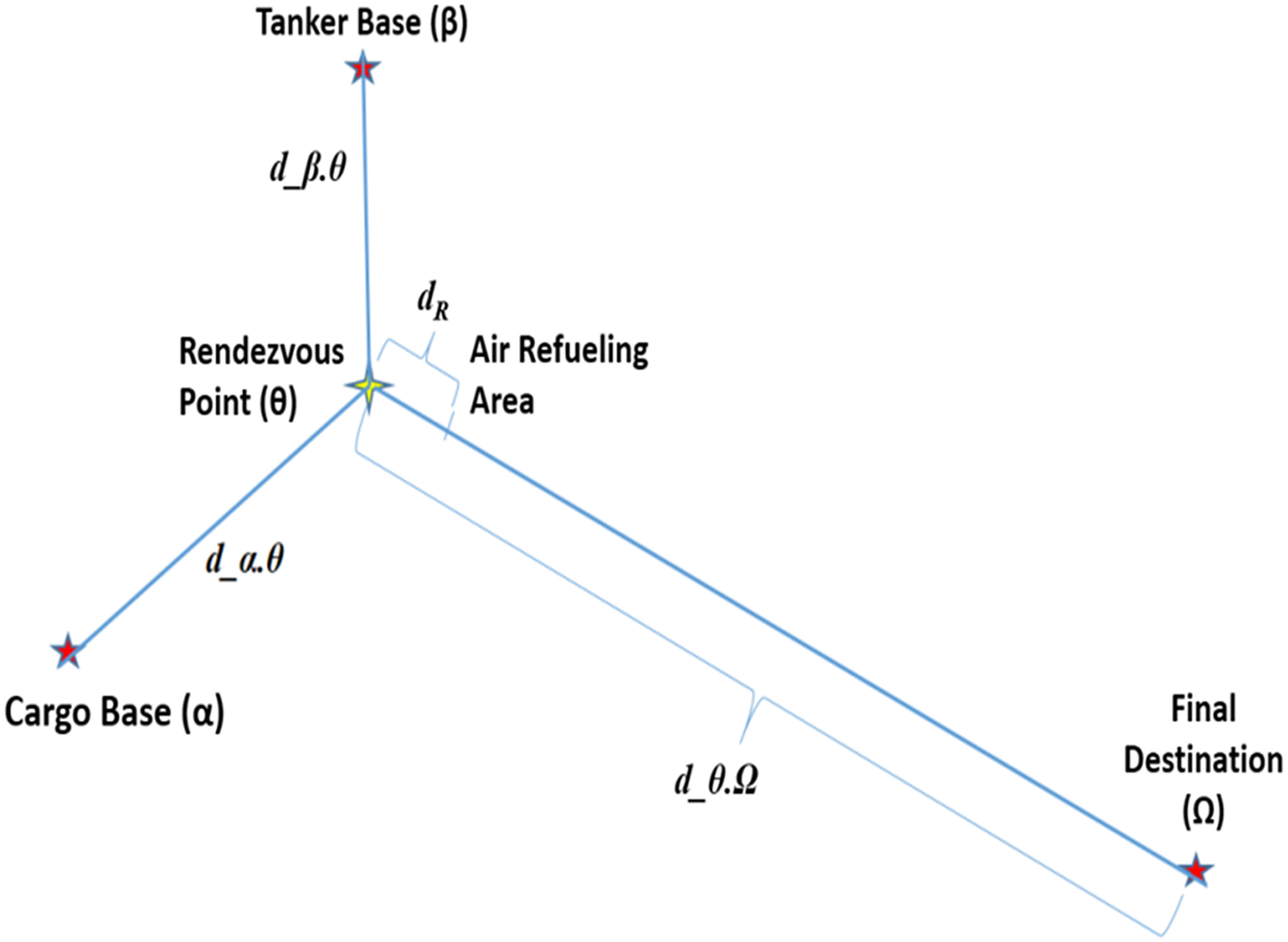
Figure 1. Flight legs.
3.3 Aircraft fuel planning
An aircraft’s fuel requirements, for a given mission, can be divided into the following components:
-
• Start, taxi, auxiliary power unit, takeoff: This fuel is consumed. The respective amounts are provided in manufacturers’ flight manual performance data and fuel planning documents as fixed values.
-
• Reserve: 10% of the flight-time fuel (not to exceed one hour of fuel at normal cruise).
-
• Alternative: Fuel to fly from the destination to a point above an alternative airport if the destination airport is closed because of weather or an accident.
-
• Holding: Fuel for possible waiting in the air because of traffic congestion at the alternative location.
Note that reserve, alternative and holding fuel are for long delays or visibility issues in poor weather conditions. In this study, no such conditions are assumed, so reserve, alternative and holding fuel is carried but not used.
-
• Climb: The fuel consumed during climb to cruise altitude. We assume that both cargo and tanker aircraft cruise at the same altitude.
-
• Cruise: Fuel consumed while an aircraft maintains its cruise altitude. Since aircraft weight changes over time, the cruise fuel burn rate also changes. We use Equations 3 and 4 to calculate the cruise fuel.
We combine descent, approach and landing fuel with cruise fuel to mitigate model complexity. Since actual descent, approach and landing fuel usage does not exceed (and is typically less than) cruise fuel consumption, our model yields conservative results.
4.0 MODEL BUILDING
A nonlinear mixed integer model for the air refueling option (P1) and a nonlinear model for without the air refueling option (P2) are constructed. Model (P1) inputs include the geographic coordinates of the tanker base, cargo aircraft origin and final destination, and the total freight weight to be moved. It then computes the optimal geographic location of the rendezvous point at which air refueling begins, the initial fuel and freight amount loaded to each cargo aircraft and the total number of required tanker and cargo aircraft sorties, to minimise the overall time taken to conduct the airlift. Moreover, total fuel consumption and the minimum number of required cargo aircraft are calculated based on the model output. Model (P2) optimises the payload of each transport aircraft to move the same total freight from origin to destination, to minimise the overall time to conduct the airlift without air refueling. We finish by comparing total airlift times for P1 and P2.
We adopted Toydas and Saraç’s(Reference Toydas and Saraç17) methodology for calculating distances and transforming trigonometric functions into a polynomial form. As Toydas and Saraç(Reference Toydas and Saraç17) did, all distances are calculated as great circle distances by using the haversine formula, and a Taylor series approximation is used to transform the trigonometric functions into a polynomial form in order to ease the model’s nonlinearity. We used the same parameter values as Toydas(Reference Toydas16) regarding C-5 and KC-10 aircraft. Other required parameters concerning the aircraft and flight planning were obtained from applicable U.S. Air Force aircraft technical documentation(21,22) , and the U.S. Air Force Air Mobility Planning Factors pamphlet(23). See Appendix A for all of the parameter values.
4.1 Haversine distance formula
The haversine distance formula gives the great-circle distance between two points s and f on a sphere, given their longitudes and latitudes. First, the interior spherical angle (
 $\Delta\sigma$
) is calculated using Equation (5). Then,
$\Delta\sigma$
) is calculated using Equation (5). Then,
 $\Delta\sigma$
is multiplied by the radius of the Earth (3440.1 NM) to yield the great-circle distance between two locations.
$\Delta\sigma$
is multiplied by the radius of the Earth (3440.1 NM) to yield the great-circle distance between two locations.
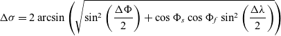 \begin{align}\Delta \sigma = 2{\rm{\;arcsin}}\left( {\sqrt {{\rm{si}}{{\rm{n}}^2}\left( {\frac{{\Delta \Phi }}{2}} \right) + {\rm{cos\;}}{\Phi _s}{\rm{\;cos\;}}{\Phi _f}{\rm{\;si}}{{\rm{n}}^2}\left( {\frac{{\Delta \lambda }}{2}} \right)} } \right)\end{align}
Where,
 $\Delta\sigma$
: Interior Spherical Angle (radians) ΔΦ: difference between latitudes (radians)
$\Delta\sigma$
: Interior Spherical Angle (radians) ΔΦ: difference between latitudes (radians)
Φ s : Latitude of point s (radians) Φ f : Latitude of point f (radians)
 $\Delta\lambda$
: difference between longitudes (radians)
$\Delta\lambda$
: difference between longitudes (radians)
4.2 Taylor series approximation
P1, which is a mixed integer nonlinear minimisation problem with a nonlinear objective function and constraints along with binary variables, is heavily nonlinear even without trigonometric functions in it. This is one of the hardest optimisation problem types. Having variables and constraints with complex trigonometric functions makes it even harder, if not impossible, to solve with available solvers. Moreover, some solvers, like Dicopt and Conopt, do not support some of the trigonometric functions such as the arcsin function where some, like Baron, do not support any trigonometric functions at all. Hence, in order to ease these difficulties, the following Taylor series are used to transform functions in the haversine formula into polynomial approximations:
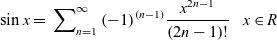 \begin{align}\sin x = \;\sum\nolimits_{n = 1}^\infty {{{\left( { - 1} \right)}^{\left( {n - 1} \right)}}} {{{x^{2n - 1}}} \over {\left( {2n - 1} \right)!}}\,\,\,\,x \in R\end{align}
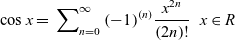 \begin{align}\cos x = \;\sum\nolimits_{n = 0}^\infty {{{\left( { - 1} \right)}^{\left( n \right)}}} {{{x^{2n}}} \over {\left( {2n} \right)!}}\,\,\,x \in R\end{align}
 \begin{align}\arcsin x = \;\;\;\sum\nolimits_{n = 0}^\infty \; {{\left( {2n} \right)!} \over {{2^{2n}}{{\left( {n!} \right)}^2}}}\;\;{{{x^{2n + 1}}} \over {\left( {2n + 1} \right)}}\,{\rm{which}}\;{\rm{converges}}\;{\rm{when}}\; - 1 \le x \le 1\end{align}
The corresponding partial series approximate the actual trigonometric functions, with higher-degree polynomials yielding more accurate values. However, there is a trade-off between solution complexity and accuracy. So, in order to find the simplest approximations which yield sufficient accuracy in the haversine formula, different approximations have been examined for each function, leading us to select the 7th-degree Taylor polynomial for sin x, 5th-degree for cos x, and 9th-degree for arcsin x (Reference Toydas and Saraç17).
4.3 Assumptions and notation
Assumptions
-
• n aircraft are loaded with freight simultaneously at the point of origin (with n depending on available ramp space at the airport). Right after loading is completed for the first n cargo aircraft, loading of the next n cargo aircraft starts.
-
• The ramp capacity is assumed to accommodate the same number (n) of aircraft at both origin and destination. If not, the smaller capacity is taken to be n for both locations.
-
• Enough equipment and personnel are available to load/offload cargo aircraft on the ground all the time.
-
• There are enough crew (pilots, loadmasters, boom operators) to fly all cargo and tanker aircraft.
-
• There are enough cargo and tanker aircraft available at hand.
-
• Each cargo aircraft is loaded with the same freight weight and initial fuel.
-
• Air refueling begins at the same rendezvous point for each aircraft. n cargo aircraft can be air-refueled simultaneously at the rendezvous point by n tankers, with flight safety guaranteed through lateral separation.
-
• Air refueling is performed at cruise speed and cruise altitude.
-
• There are no cargo load balance or size restrictions.
-
• Aircraft scheduling is perfect. No aircraft are late to a refueling event.
-
• The earth is a perfect sphere and aircraft follow great circle routes.
-
• Winds at altitude are negligible. Temperature and other weather considerations represent standard conditions as noted in associated technical orders or performance documents.
-
• Both cargo and tanker aircraft cruise at 31,000 feet. The a 0 and a 1 constants, which are used in Equations 1–4, are derived for this altitude.
-
• During air refueling, the tanker and cargo aircraft fuel burn rates are equal to their respective cruise fuel burn rates and do not change due to transferred fuel weight or deployed tanker boom drag.
-
• If a tanker aircraft’s remaining off-loadable fuel is less than the cargo aircraft’s need, then the tanker off-loads all its off-loadable fuel. Another tanker immediately gets in position and off-loads the remaining required fuel. The time required for formation changes is negligible.
-
• Cargo aircraft carry no cargo while returning from destination to origin. Thus, the fuel consumed during return is considered in the model as waste when calculating the total fuel savings.
Notation
Set
- j
-
Aircraft Type (as superscript: C=Cargo Aircraft, T=Tanker Aircraft)
Decision Variables
-
 $\boldsymbol\theta$
-
Cargo aircraft air refueling start point (Represented as latitude
$\boldsymbol\theta$
_
lat, and longitude
$\theta$
_
long in the model) - g
-
Initial cargo aircraft fuel load (lbs)
- w
-
Freight weight loaded on each cargo aircraft (lbs)
- w Last
-
Freight weight loaded to last cargo aircraft in problem P2 (lbs)
- g off
-
Amount of fuel offloaded to each cargo aircraft from tanker aircraft
- N C
-
Number of cargo aircraft sorties needed to move total freight
- N T
-
Number of tanker aircraft sorties needed to refuel N C
- Q
-
Number of cargo aircraft that can be refueled by one tanker aircraft
- d_x.y
-
Great circle distance between x and y generic locations calculated with haversine formula (Instead of generic x and y points, necessary geographic locations are used in the model. For example, d_
$\theta$
.Ω shows the great circle distance between first air refueling point and destination point calculated from
$\theta\!$
_
lat,
$\theta\!$
_
long
, Ω_
lat
, Ω_
long.) - d R
-
Distance traversed during air refueling
- FC j [(g),(w),(d)]
-
Fuel consumed when a type j aircraft flies a distance d, its initial fuel is g and its cargo freight weight is w; using Equation 3. (These three parameters of the function are manipulated as required for the fuel calculations in the model.)
- FR j [(w),(d)]
-
Fuel required by a type j aircraft to fly a distance d, when freight cargo weight is w; using Equation 4. (These two parameters of the function are manipulated as required for the fuel calculations in the model.)
-
$$t_A^C$$
-
Total flight time of each cargo aircraft for the air refueling option
-
$$t_N^C$$
-
Total flight time of each cargo aircraft for the direct flight without air refueling option
- Y1
-
Total fuel consumption from problem P1
- Y2
-
Total fuel consumption from problem P2
-
$${T_1}$$
-
Total airlift time of P1 to move total freight
-
$${T_2}$$
-
Total airlift time of P2 to move total freight


Parameters
- EW j
-
Type j aircraft empty weight
- MTOW j
-
Type j aircraft maximum takeoff weight
- MWA C
-
Cargo aircraft maximum weight in the air
- R j
-
Type j aircraft reserve + alternate + holding fuel
- S j
-
Type j aircraft start + taxi + takeoff fuel
- C j
-
Type j aircraft climb fuel
- Crg C
-
Cargo aircraft total cargo capacity
- K j
-
Type j aircraft total fuel capacity
- F T
-
Maximum fuel amount that can be loaded to a tanker aircraft on the ground
- B T
-
Approximate fuel burn rate of tanker aircraft (lbs/hr)
- H T
-
Tanker aircraft approximate speed during air refueling
- h
-
Tanker aircraft boom fuel transfer rate (lbs/hr)
- TW
-
Total freight weight to be moved from cargo base to destination
- n
-
Number of cargo aircraft that can be loaded simultaneously on the ground at the point of origin
-
$\boldsymbol\alpha$
-
Geographical coordinates of the cargo base (represented as latitude and longitude)
-
$\boldsymbol\beta$
-
Geographical coordinates of the tanker base (represented as latitude and longitude)
-
$\boldsymbol\Omega$
-
Geographical coordinates of the destination point (represented as latitude and longitude)
-
$$d_{TC}^J$$
-
Distance traversed during takeoff and climb by type j aircraft
-
$$V_C^C$$
-
Cruise speed of cargo aircraft
-
$$V_R^C$$
-
Air refueling speed of cargo aircraft
-
$$G_L^C$$
-
Ground time of cargo aircraft for freight load operation
-
$$G_O^C$$
-
Ground time of cargo aircraft for freight offload operation


4.3.1 Problem formulation
Cargo aircraft fuel calculations
The fuel needed by each cargo aircraft for the air refueling option is composed of three components.
The first component is the fuel consumed from takeoff at α to the air refueling start point
 $\theta$
, at a distance d_α.
$\theta$
, at a distance d_α.
 $\theta$
:
$\theta$
:
 \begin{align}{S^C} + {C^C} + F{C^C}\left[ {\left( {g - {S^C} - {C^C}} \right),\left( w \right),\left( {d\_\alpha .\theta - d_{TC}^C} \right)} \right]\end{align}
As mentioned earlier in the notation section, FC
C
function has three parameters, which are the initial fuel g, the initial freight w, and the distance to be flown d. These parameters are manipulated for the fuel calculations. Note that
 $d_{TC}^C$
is excluded from the distance flown since the fuel consumed during climb,
$d_{TC}^C$
is excluded from the distance flown since the fuel consumed during climb,
 ${C^C}$
, which is a fixed amount, is already included in the fuel consumption on this leg. In this case, the remaining total fuel on board the cargo aircraft is:
${C^C}$
, which is a fixed amount, is already included in the fuel consumption on this leg. In this case, the remaining total fuel on board the cargo aircraft is:
 \begin{align}g - \left( {{S^C} + {C^C} + F{C^C}\left[ {\left( {g - {S^C} - {C^C}} \right),\left( w \right),\left( {d\_\alpha .\theta - d_{TC}^C} \right)} \right]} \right)\end{align}
Note that reserve, alternative and holding fuel are for long delays or visibility issues in poor weather conditions. In this study, no such conditions are assumed, so reserve, alternative and holding fuel are carried but not used. So, the remaining usable fuel on board the ith cargo aircraft is
 $\left( {10} \right) - {R^C}$
, i.e.
$\left( {10} \right) - {R^C}$
, i.e.
 \begin{align}g - \left( {{S^C} + {C^C} + F{C^C}\left[ {\left( {g - {S^C} - {C^C}} \right),\left( w \right),\left( {d\_\alpha .\theta - d_{TC}^C} \right)} \right]} \right){\rm{\;}} - {R^C}\end{align}
The second component is the fuel required to fly from the air refueling point
 $\theta$
to destination
$\theta$
to destination
 $\Omega$
over a distance d_
$\Omega$
over a distance d_
 $\theta.\Omega$
 \begin{align}F{R^C}\left[ {\left( {w + {R^C}} \right),\left( {d\_\theta .\Omega } \right)} \right]\end{align}
Note that the first parameter of the fuel requirement function, w, is considered as w+R C , because R C represents fuel that, though not used, is carried just like w.
(12) should also be equal to:
 $\;g + {g_{{\rm{off}}}} - {R^C} - {S^C} - {C^C} - F{C^C}\left[ {\left( {g - {S^C} - {C^C}} \right),\left( w \right),}\right.$
 ${\left.\left( {d\_\alpha .\theta - d_{TC}^C} \right) \right])}$
to make sure that remaining usable fuel on board at the rendezvous point plus offloaded fuel during air refueling is enough to fly from rendezvous point to the final destination. This will be guaranteed with a constraint in the model.
${\left.\left( {d\_\alpha .\theta - d_{TC}^C} \right) \right])}$
to make sure that remaining usable fuel on board at the rendezvous point plus offloaded fuel during air refueling is enough to fly from rendezvous point to the final destination. This will be guaranteed with a constraint in the model.
The fuel amount that should be offloaded from the tanker to the cargo aircraft during air refueling:
 ${g_{off}}_i = \left( {12} \right) - \left( {11} \right)$
, which means;
${g_{off}}_i = \left( {12} \right) - \left( {11} \right)$
, which means;
 \begin{align}{g_{{\rm{off}}}} &= F{R^C}\left[ {\left( {w + {R^C}} \right),\left( {d\_\theta .\Omega } \right)} \right] - g + {S^C} + {C^C} \nonumber \\[3pt] &\quad + F{C^C}\left[ {\left( {g - {S^C} - {C^C}} \right),\left( w \right),\left( {d\_\alpha .\theta - d_{TC}^C} \right)} \right] + {R^C}\end{align}
Note that
 ${g_{{\rm{off}}}}_i$
does not have to be equal to Equation 12, depending on the initial fuel amount, g, which is also a decision variable.
${g_{{\rm{off}}}}_i$
does not have to be equal to Equation 12, depending on the initial fuel amount, g, which is also a decision variable.
As soon as air refueling is completed, the total fuel is
 ${g_{{\rm{off}}}}_i + \left( {10} \right)$
, i.e.
${g_{{\rm{off}}}}_i + \left( {10} \right)$
, i.e.
 \begin{align}{g_{{\rm{off}}}} + g - {S^C} - {C^C} - F{C^C}\left[ {\left( {g - {S^C} - {C^C}} \right),\left( w \right),\left( {d\_\alpha .\theta - d_{TC}^C} \right)} \right]\end{align}
The third component is fuel consumed to fly back from final destination to cargo base without carrying any cargo:
 \begin{align}{S^C} + {R^C} + F{R^C}\left[ {\left( {{R^C}} \right),\left( {d\_\Omega .\alpha - d_{TC}^C} \right)} \right]\end{align}
So, total fuel consumption of each cargo aircraft is:
 $T{C^C} = \left( 9 \right) + \left( {12} \right) + \left( {15} \right)$
, which means
$T{C^C} = \left( 9 \right) + \left( {12} \right) + \left( {15} \right)$
, which means
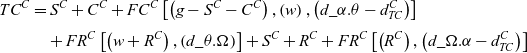 \begin{align}T{C^C} &= {S^C} + {C^C} + F{C^C}\left[ {\left( {g - {S^C} - {C^C}} \right),\left( w \right),\left( {d\_\alpha .\theta - d_{TC}^C} \right)} \right]\nonumber\\[3pt] &\quad + F{R^C}\left[ {\left( {w + {R^C}} \right),\left( {d\_\theta .\Omega } \right)} \right] + {S^C} + {R^C} + F{R^C}\left[ {\left( {{R^C}} \right),\left( {d\_\Omega .\alpha - d_{TC}^C} \right)} \right]\end{align}
Tanker aircraft fuel calculations
Tanker aircraft are assumed to take off fully loaded with fuel, so they can refuel the greatest possible number of cargo aircraft. We comment that K
T
may or may not be equal to F
T
depending upon MTOW
T
and EW
T
. Note that if
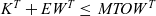 ${K^T} + E{W^T} \le \;MTO{W^T}$
, then
${K^T} + E{W^T} \le \;MTO{W^T}$
, then
 ${F^T} = {K^T}$
; otherwise,
${F^T} = {K^T}$
; otherwise,
 ${F^T} = MTO{W^T} - E{W^T}$
.
${F^T} = MTO{W^T} - E{W^T}$
.
There are three components of tanker aircraft fuel consumption. The first component is the fuel over distance d_
 $\beta\cdot\theta$
to reach the rendezvous point:
$\beta\cdot\theta$
to reach the rendezvous point:
 \begin{align}{S^T} + {C^T} + F{C^T}\left[ {\left( {{F^T} - {S^T} - {C^T}} \right),\left( 0 \right),\left( {d\_\beta .\theta - d_{TC}^T} \right)} \right]\end{align}
The second component is fuel consumption during air refueling. This amount depends on the number of cargo aircraft refueled by one tanker aircraft and the quantity of offloaded fuel. If the boom transfer rate is h (lbs/hr), it takes
 ${{2.{g_{{\rm{off}}}}} \over h}$
hours to refuel each aircraft (where the multiplier 2 reflects that the tanker flies a distance 2d
R
for each refueling event). Then, the total fuel consumption during air refueling becomes:
${{2.{g_{{\rm{off}}}}} \over h}$
hours to refuel each aircraft (where the multiplier 2 reflects that the tanker flies a distance 2d
R
for each refueling event). Then, the total fuel consumption during air refueling becomes:
 \begin{align}Q.{\rm{\;}}\frac{{2{\rm{\;}}{g_{{\rm{off}}}}}}{h}{\rm{\;}}.{B^T}\end{align}
The third component—the fuel consumed while the tanker is returning to its base across distance d_
 $\theta.\beta$
—is now addressed. The tanker will offload all its transferrable fuel and it does not carry cargo. Note that R
T
must be included on-board, and hence
$\theta.\beta$
—is now addressed. The tanker will offload all its transferrable fuel and it does not carry cargo. Note that R
T
must be included on-board, and hence
 $w = {R^T}$
, to obtain:
$w = {R^T}$
, to obtain:
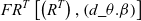 \begin{align}F{R^T}\left[ {\left( {{R^T}} \right),\left( {d\_\theta .\beta } \right)} \right]\end{align}
We can now derive Q, the number of cargo aircraft that can be refueled by one tanker:
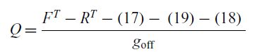 \begin{align}Q = \frac{{{F^T} - {R^T} - \left( {17} \right) - \;\left( {19} \right) - \left( {18} \right)\;}}{{{g_{{\rm{off}}}}}}\end{align}
Simplifying, we obtain:
 $$\matrix{
{Q = {{h.\left\{ {{F^T} - {R^T} - {S^T} - {C^T} - F{C^T}\left[ {\left( {{F^T} - {S^T} - {C^T}} \right),\left( 0 \right),\left( {d\_\beta .\theta - d_{TC}^T} \right)\left] { - F{R^T}} \right[\left( {{R^T}} \right),\left( {d\_\theta .\beta } \right)} \right]} \right\}} \over {{g_{{\rm{off}}}}.\left( {h + 2{B^T}} \right)}}} \hfill \cr
} $$
$$\matrix{
{Q = {{h.\left\{ {{F^T} - {R^T} - {S^T} - {C^T} - F{C^T}\left[ {\left( {{F^T} - {S^T} - {C^T}} \right),\left( 0 \right),\left( {d\_\beta .\theta - d_{TC}^T} \right)\left] { - F{R^T}} \right[\left( {{R^T}} \right),\left( {d\_\theta .\beta } \right)} \right]} \right\}} \over {{g_{{\rm{off}}}}.\left( {h + 2{B^T}} \right)}}} \hfill \cr
} $$
Cargo aircraft flight time calculations
Each cargo aircraft’s round-trip time is composed of freight loading time on the ground at the origin, flight time from origin to destination, freight offloading time on the ground at the point of destination and flight time back from destination to origin. For the air refueling option, the flight time from origin to destination incorporates the time to travel to the air refueling point form origin, and the time from there to the destination. Freight loading and offloading ground times are parameters. However, flight times depend on the distance between origin, destination and air refueling points.
The flight time from origin to destination for the air refueling option is:
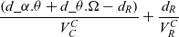 \begin{align}\frac{{\left( {d\_\alpha .\theta + d\_\theta .\Omega - {d_R}} \right)}}{{V_C^C}} + \frac{{{d_R}}}{{V_R^C}}\end{align}
Note that cruise speed and air refueling speed are different due to the procedural limitations. That is why flight time has two components.
The flight time from destination to origin is:
 \begin{align}\frac{{\left( {d\_\Omega .\alpha } \right)}}{{V_C^C}}\end{align}
The total flight time of each cargo aircraft, for the air refueling option, is thus:
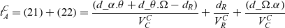 \begin{align}t_A^C = \left( {21} \right) + \left( {22} \right) = \frac{{\left( {d\_\alpha .\theta + d\_\theta .\Omega - {d_R}} \right)}}{{V_C^C}} + \frac{{{d_R}}}{{V_R^C}} + \frac{{\left( {d\_\Omega .\alpha } \right)}}{{V_C^C}}\end{align}
As mentioned earlier, we assume that n aircraft can be loaded simultaneously at the point of origin. Right after freight loading is completed for the first n cargo aircraft, the loading of the next n cargo aircraft starts. This assumption implies that the difference between freight loading start time—and also takeoff time—of two consecutive n cargo aircraft is
 $G_L^C$
at the point of origin. Moreover, if loading starts at time t=0, the first group of n aircraft take off at time 0+
$G_L^C$
at the point of origin. Moreover, if loading starts at time t=0, the first group of n aircraft take off at time 0+
 $G_L^C,$
arrive at the destination at
$G_L^C,$
arrive at the destination at
 $G_L^C + \left( {21} \right)$
, take off again to return to origin at
$G_L^C + \left( {21} \right)$
, take off again to return to origin at
 $G_L^C + \left( {21} \right) + G_O^C$
, and arrive at origin at
$G_L^C + \left( {21} \right) + G_O^C$
, and arrive at origin at
 $G_L^C + \left( {21} \right) + G_O^C + \left( {22} \right).$
The second group of n cargo aircraft takes off at
$G_L^C + \left( {21} \right) + G_O^C + \left( {22} \right).$
The second group of n cargo aircraft takes off at
 $2G_L^C$
and follows the same pattern.
$2G_L^C$
and follows the same pattern.
Hence, the total time required to move TW from origin to destination for the air refueling option is:
 \begin{align}{T_1} = \frac{{\left( {{N^c}.G_L^C} \right) + t_A^C + G_O^C}}{n}\end{align}
Considering that each group of n cargo aircraft takes off
 $G_L^C$
hours apart, the round-trip flight time between origin and destination takes
$G_L^C$
hours apart, the round-trip flight time between origin and destination takes
 $t_A^C$
hours for the air refueling option, and the total number of cargo aircraft required to move TW from origin to destination for the air refueling option is
$t_A^C$
hours for the air refueling option, and the total number of cargo aircraft required to move TW from origin to destination for the air refueling option is
 \begin{align}\left( {\frac{{t_A^C}}{{G_L^C}} + 1} \right).n\end{align}
P1 model
We can now define problem P1, which minimises the total time required to move TW from origin to destination as:
 ${\rm{P}}1:{\rm{\;Minimise\;}}{T_1}$
subject to:
${\rm{P}}1:{\rm{\;Minimise\;}}{T_1}$
subject to:
 \begin{align}w.{N^C} \ge\ TW\end{align}
 \begin{align}\frac{{\;{N^C}}}{Q} - {N^T} \le 0\end{align}
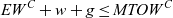 \begin{align}E{W^C} + w + g \le MTO{W^C}\end{align}
 \begin{align}g \le {K^C}\end{align}
 \begin{align}F{R^C}\left[ {\left( {w + {R^C}} \right),\left( {d\_\theta .\Omega } \right)} \right] + {{\rm{R}}^{\rm{C}}} \le {{\rm{K}}^{\rm{C}}}\end{align}
 \begin{align}w{\rm{\;}} \le {\rm{\;}}Cr{g^C}\end{align}
 \begin{align}E{W^C} + w + F{R^C}\left[ {\left( {w + {R^C}} \right),\left( {d\_\theta .\Omega } \right)} \right] + {R^C} \le MW{A^C}\end{align}
 \begin{align}d\_\beta .\theta - d_{TC}^T \ge 0\end{align}
 \begin{align}d\_\alpha .\theta - d_{TC}^C \ge 0\end{align}
 \begin{align}g \ge {S^C} + {C^C} + F{C^C}\left[ {\left( {g - {S^C} - {C^C}} \right),\left( w \right),\left( {d\_\alpha .\theta - d_{TC}^C} \right)} \right]\end{align}
 \begin{align}&g + {g_{off}} - {R^C} - {S^C} - {C^C} - F{C^C}\left[ {\left( {g - {S^C} - {C^C}} \right),\left( w \right),\left( {d\_\alpha .\theta - d_{TC}^C} \right)} \right]) \nonumber\\ &\ge F{R^C}\left[ {\left( {w + {R^C}} \right),\left( {d\_\theta .\Omega } \right)} \right]\end{align}
 \begin{align}{S^C} + {R^C} + F{R^C}\left[ {\left( {{R^C}} \right),\left( {d\_\Omega .\alpha - d_{TC}^C} \right)} \right] \le {{\rm{K}}^{\rm{C}}}\end{align}
 \begin{align} - \frac{\pi }{2} \le \theta \_{\rm{lat}} \le {\rm{\;}}\frac{{\rm{\pi }}}{2}\end{align}
 \begin{align} - \pi \le \theta \_{\rm{long}} \le \;\pi \end{align}
 \begin{align}g, w, N^C, N^T \ge 0\end{align}
 \begin{align}N^C, N^T \textrm{integer}\end{align}
Constraint (P1.1) guarantees that all of the freight is moved, while (P1.2) forces the tanker aircraft to perform the air refueling. Constraint (P1.3) prevents a loaded cargo aircraft from exceeding its maximum takeoff weight limit. Constraints (P1.4) and (P1.5) preclude the respective initial on-ground and post-air-refueling fuel capacities from exceeding the cargo aircraft’s storage limits. Constraint (P1.6) prevents the cargo aircraft from being overloaded, while (P1.7) assures that the cargo aircraft gross weight right after air refueling does not exceed the aircraft’s total allowable weight in the air. Since climb fuel is a parameter, the distance d
TC
is excluded on legs d_α.
 $\theta$
and d_
$\theta$
and d_
 $\beta.\theta$
while calculating fuel consumption on these legs. Constraints (P1.8) and (P1.9) prevent negative distance values so that the fuel consumption functions work properly. These two constraints together force the rendezvous point to be optimised at least d
TC
miles away from the tanker and cargo bases. Constraint (P1.10) requires the cargo aircraft to obtain enough initial fuel to reach the rendezvous point while constraint (P1.11) ensures that the usable fuel on board right after refueling is enough to reach the final destination. Constraint (P1.12) assures that the total fuel on board while the cargo aircraft is flying back empty is less than its maximum fuel capacity. Constraints (P1.13) and (P1.14) provide latitudes and longitude boundaries. Constraints (P1.15) and (P1.16) enforce non-negativity and integrality conditions on the respective variables. Note that
$\beta.\theta$
while calculating fuel consumption on these legs. Constraints (P1.8) and (P1.9) prevent negative distance values so that the fuel consumption functions work properly. These two constraints together force the rendezvous point to be optimised at least d
TC
miles away from the tanker and cargo bases. Constraint (P1.10) requires the cargo aircraft to obtain enough initial fuel to reach the rendezvous point while constraint (P1.11) ensures that the usable fuel on board right after refueling is enough to reach the final destination. Constraint (P1.12) assures that the total fuel on board while the cargo aircraft is flying back empty is less than its maximum fuel capacity. Constraints (P1.13) and (P1.14) provide latitudes and longitude boundaries. Constraints (P1.15) and (P1.16) enforce non-negativity and integrality conditions on the respective variables. Note that
 $\theta$
_lat,
$\theta$
_lat,
 $\theta$
_long, g and w are the independent decision variables while the other decision variables are dependent variables, calculated from the independent ones.
$\theta$
_long, g and w are the independent decision variables while the other decision variables are dependent variables, calculated from the independent ones.
Moreover, based on the output of P1, the total fuel consumption can be calculated as:
 \begin{align}Y1 = {N^C}.\left[ {\left( 9 \right) + \left( {12} \right) + \left( {15} \right)} \right] + {N^T}.\left[ {\left( {17} \right) + \left( {18} \right) + \left( {19} \right)} \right]\end{align}
P2 model
This model assumes that the total freight is moved by cargo aircraft without air refueling. So, w is the only decision variable, and all cargo aircraft carry the same load weight w. In this case, the total number of cargo aircraft required to move the total freight is:
 \begin{align}{N^c} = \left\lceil\frac{{TW}}{w}\right\rceil\end{align}
Depending on w and TW, the last cargo aircraft’s freight load is either equal or less that the other cargo aircraft’s freight load. So,
 \begin{align}{w_{{\rm{Last}}}} = {\rm{TW}} - \left[ {\left( {{{\rm{N}}^{\rm{C}}} - 1} \right).w} \right]\end{align}
Flight time from origin to destination, and from destination to origin, is:
 \begin{align}\frac{{\left( {d\_\alpha .\Omega } \right)}}{{V_C^C}}\end{align}
The total flight time of each cargo aircraft is:
 \begin{align}t_N^C = \frac{{2.\left( {d\_\alpha .\Omega } \right)}}{{V_C^C}}\end{align}
Hence, the total time required to move TW from origin to destination is:
 \begin{align}{T_2} = \frac{{\left( {{N^c}.G_L^C} \right) + t_N^C + G_O^C}}{n}\end{align}
The total number of cargo aircraft required, without air refueling, is:
 \begin{align}\left(\left\lceil \frac{{t_N^C}}{{G_L^C}}\right\rceil + 1.n\right)\end{align}
The total fuel consumption of all cargo aircraft is:
 \begin{align}Y2 &= {S^C} + {C^C} + F{R^C}\left[ {\left( {{w_{Last}} + {R^C}} \right),\left( {d\_\alpha .\Omega - d_{TC}^C} \right)} \right] \nonumber\\[3pt]
&\quad + \left( {{N^C} - 1} \right)\times
\left( {S^C} + {C^C} + F{R^C}\left[ \left( {w + {R^C}} \right),( d\_\alpha .\Omega - d_{TC}^C) \right] \right) \nonumber\\[3pt] &\quad + {N^C}.({S^C} + {C^C} + F{R^C}\left[ ({R^C} ),\left( {d_{\alpha} .\Omega - d_{TC}^C} \right) \right])\end{align}
\begin{align}Y2 &= {S^C} + {C^C} + F{R^C}\left[ {\left( {{w_{Last}} + {R^C}} \right),\left( {d\_\alpha .\Omega - d_{TC}^C} \right)} \right] \nonumber\\[3pt]
&\quad + \left( {{N^C} - 1} \right)\times
\left( {S^C} + {C^C} + F{R^C}\left[ \left( {w + {R^C}} \right),( d\_\alpha .\Omega - d_{TC}^C) \right] \right) \nonumber\\[3pt] &\quad + {N^C}.({S^C} + {C^C} + F{R^C}\left[ ({R^C} ),\left( {d_{\alpha} .\Omega - d_{TC}^C} \right) \right])\end{align}
In this case, P2 is as following:
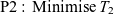 ${\rm{P}}2:{\rm{\;Minimise\;}}{T_2}$
subject to:
${\rm{P}}2:{\rm{\;Minimise\;}}{T_2}$
subject to:
 \begin{align}{{\rm{S}}^{\rm{C}}} + {{\rm{C}}^{\rm{C}}} + {\rm{F}}{{\rm{R}}^{\rm{C}}}\left[ {\left( {w + {{\rm{R}}^{\rm{C}}}} \right),\left( {d\_\alpha .\Omega - d_{TC}^C} \right)} \right] + {{\rm{R}}^{\rm{C}}} + {\rm{E}}{{\rm{W}}^{\rm{C}}} + w \le {\rm{MTO}}{{\rm{W}}^{\rm{C}}}\end{align}
 \begin{align}{{\rm{S}}^{\rm{C}}} + {{\rm{C}}^{\rm{C}}} + {\rm{F}}{{\rm{R}}^{\rm{C}}}\left[ {\left( {w + {{\rm{R}}^{\rm{C}}}} \right),\left( {d\_\alpha .\Omega - d_{TC}^C} \right)} \right] + {{\rm{R}}^{\rm{C}}} \le {{\rm{K}}^{{\rm{C\;}}}}\end{align}
 \begin{align}w \le Crg^C\end{align}
Constraint (P2.1) limits the maximum takeoff weight. (P2.2) limits available fuel capacity, while (P2.3) limits overall cargo capacity per cargo aircraft. Consequently, if
 ${T_1} \lt {T_2}$
, then the air refueling option is practicable. Otherwise, it is impracticable.
${T_1} \lt {T_2}$
, then the air refueling option is practicable. Otherwise, it is impracticable.
5.0 NUMERICAL EXAMPLE
We illustrate our models on a numerical example with a mid-range origin–destination pair. C-5 cargo aircraft and KC-10 tanker aircraft are selected for the scenario. The model was run for various numbers of cargo aircraft that can be loaded simultaneously on the ground (n), and two tanker base locations, to capture the relationship between these inputs and total airlift time.
We coded and solved P1 and P2 in the General Algebraic Modeling System (GAMS). P1 is a mixed-integer nonlinear programming (MINLP) problem, and P2 is a nonlinear programming (NLP) problem. We used the GAMS DICOPT (Discrete and Continuous Optimiser) program for the MINLP problem. The MINLP algorithm in DICOPT solves a series of NLP and MIP (Mixed-Integer Programming) sub-problems. These sub-problems can be solved using any NLP or MIP solver that runs under GAMS. We used the GAMS CONOPT and GAMS/Cplex solvers for NLP and MIP, respectively. Solution time is under two minutes for P1 and under 30 seconds for P2. The parameters for the C-5 and KC-10 aircraft are given in Appendix A. We reached a local optimum solution for P1 and ran the P1 model multiple times to investigate the solution’s robustness and to see that GAMS returned consistent solutions. We got a global optimum solution for P2. Since P1 is heavily nonlinear and we see that substantial savings are possible, we are satisfied with the local optimum solution. However, potential savings may be even greater than the values we report.
Table 1 Geographic coordinates of the bases for the first scenario

Considering current and potential future conflicts in the Middle East, we choose Ramstein Air Base in Germany as the origin and Al Udeid Air Base in Qatar as the destination. Ramstein Air Base is the largest U.S Air Force base in Europe and the main hub for Middle East and Afghanistan deployments. On the other hand, Al Udeid Air Base is a large logistics hub in Qatar that can accommodate more than 10,000 troops and 120 aircraft. Moreover, it is in close proximity to ongoing or potential conflict areas such as Syria, Yemen, Iraq, Iran etc., and is hence a good candidate for a forward supply point. The distance from the cargo base to the final destination is 2,496 nautical miles.
Mahan et al.(Reference Mahan, Key, Reckamp and Brigantic24) noted: “In October 1999, the Army’s Chief of Staff issued a vision statement to transform the service, including the goal of deploying a combat force anywhere in the world within 96 hours after liftoff. Their target is to have the entire interim brigade combat team (IBCT) deploy within 96 hours of first aircraft wheels-up.”
Table 2 Scenario results
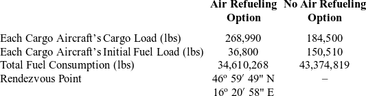
Table 3 Scenario results
In our numerical example, we evaluated the Army’s IBCT deployment vision for The Stryker brigade for our origin–destination pair in terms of total airlift time and the number of aircraft required. The Stryker brigade, which is a mechanised infantry force structured around the Stryker eight-wheeled vehicle, has about 1,500 wheeled vehicles, almost 3,900 soldiers, and three days of supplies, for a total of 14,660 short tons of material—equal to 29,320,000 lbs.
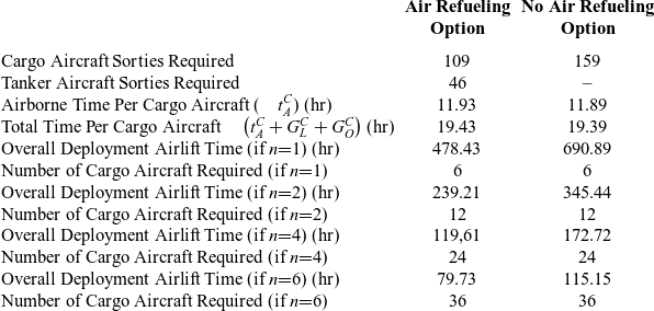
Tables 2 and 3 depict scenario outputs. It requires 109 C-5 cargo sorties and 54 KC-10 fuel sorties to move 29,320,000 lbs. of freight from Ramstein Air base to Al Udeid Air Base if the proposed air refueling operation is conducted. Without air refueling, 159 C-5 sorties are required. If only one C-5 at a time can be loaded at the origin (i.e. n=1), the total airlift time (T 1 ) is 478.42 hours with air refueling, or (T 2 ) 690.89 hours without air refueling. Six cargo aircraft are required to conduct this airlift operation if n=1. In this case, air refueling saves 212.42 hours. However, we know that both Ramstein and Al Udeid Air Bases have more ramp space to load/off-load multiple cargo aircraft simultaneously. For example; if 4 aircraft are loaded/off-loaded simultaneously, overall deployment airlift time drops to 119.61 hours with air refueling and 172.72 hours without air refueling. In this case, air refueling saves 53.11 hours, and 24 cargo aircraft are required to conduct this deployment operation. The U.S. Army’s goal of deploying a brigade within 96 hours is possible with air refueling if 6 cargo aircraft can be loaded/offloaded simultaneously. To achieve this goal, we need 36 cargo and 36 tanker aircraft.
As one can see above, air refueling can shorten overall airlift time substantially for large-scale deployments. In addition to that, it can also result in a considerable saving of fuel. The total fuel savings from the reduced number of cargo sorties, due to air refueling, surpasses the extra fuel consumed by the tanker sorties. Even though extra fuel is consumed due to the tanker flights, the reduced number of cargo sorties yields a lower total fuel consumption compared with the no-air refueling option. In our example, total fuel consumption is 34.6 million pounds with air refueling, compared with 43.4 million pounds without air refueling (see Table 2), so air refueling would save 6.8 million pounds of fuel in addition to the considerable saving of airlift time.
We also investigate this scenario for another tanker base location. For a Europe–Middle East deployment scenario, Incirlik Air Base, in southern Turkey (37º 00
 $^{\prime}$
07" N, 35º 25
$^{\prime}$
07" N, 35º 25
 $^{\prime}$
33" E), is a potential tanker base candidate. This change of tanker base results in the same reductions in total airlift time and aircraft requirements, and also yields a slight decrease in total fuel consumption: using Incirlik as the tanker base for this deployment scenario resulted in 34,338,049.40 pounds of total fuel consumption, which is 272,219.01 pounds less.
$^{\prime}$
33" E), is a potential tanker base candidate. This change of tanker base results in the same reductions in total airlift time and aircraft requirements, and also yields a slight decrease in total fuel consumption: using Incirlik as the tanker base for this deployment scenario resulted in 34,338,049.40 pounds of total fuel consumption, which is 272,219.01 pounds less.
6.0 CONCLUSION
In this study, we investigate whether air refueling can shorten the total time of an airlift operation and decrease the number of cargo aircraft sorties required in a deployment scenario, when the distance between origin and destination is within the range of cargo aircraft. We introduced two mathematical models to compare the total airlift time and the number of cargo aircraft required for given origin, destination and tanker base locations and the total freight to be moved. We optimised initial cargo and fuel amount for cargo aircraft along with rendezvous point coordinates to minimise total airlift time.
Our results show that substantial airlift time and cargo aircraft sortie savings are possible through air refueling. Moreover, air refueling can save a substantial amount of fuel due to the reduced number of cargo sorties. Our findings prove that more agile, efficient military deployments with a lower carbon footprint are possible if air refueling is conducted even for within-range origin–destination pairs.
We conducted interviews with KC-10 and C-5 pilots to validate our model. Based on their expert opinion and further comparison with Advanced Computer Flight Plan (ACFP) software results, which the U.S. Air Force Air Mobility Command (AMC) uses for actual fuel requirement planning, they concluded that our fuel consumption calculations and results are realistic and in agreement with the actual fuel calculations.
Single types of cargo and tanker aircraft were selected for this study. Studying heterogeneous cargo and tanker fleets which utilise more than one type of aircraft at the same time (e.g. C-5, C-17 and C-130 types for the cargo aircraft, KC-10 and KC-135 for the tanker aircraft, etc.) would be one possible future research area. Moreover, the single origin and destination specifications can be expanded to a network with multiple origins, destinations, and tanker bases, for further investigation.
7.0 DISCLAIMER
The views expressed are those of the authors, and do not reflect the position or policy of the United States Air Force, Department of Defense, the United States Government, Turkish Air Force, Turkish Ministry of National Defense, or Turkish Government.
APPENDIX A. AIRCRAFT FACTS SUMMARY TABLE
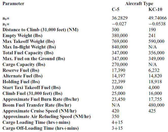
This data is compiled from Toydaş(Reference Toydas16), operations procedures volume-3 documents of C-5 and KC-10 aircraft(21,22) , AFPAM 10-1403 Air Mobility Planning Factors(23) and Fact Sheets for each aircraft published at the official U.S Air Force web site (www.af.mil).
Table A-1 Aircraft facts summary table


 Open access