


1. Introduction
Reliable prediction of the erosion of non-cohesive sediment is important for assessment of the safety level of levees, prediction of coastal erosion, and optimization of dredging methods and equipment. Also, this information is important for the understanding of river systems and fluvial landforms. Although there exist several theoretical attempts to address the erosion problem (Cao Reference Cao1997; Zhong, Wang & Ding Reference Zhong, Wang and Ding2011), understanding is still far from satisfactory, and the proposed scaling relations are mainly empirical.
The vertical particle flux from a sediment bed is defined as  $F(y)=\rho _p\,\langle \alpha v_p\rangle$, where $\rho _p$ is the density of the solid particles, $\alpha$ is the instantaneous solid phase fraction, $v_p$ is the instantaneous vertical velocity of the particle phase obtained by volume averaging, and the brackets $\langle \cdot \rangle$ denote the Reynolds average, i.e. an ensemble average over multiple realizations of the flow (Pope Reference Pope2000). It is helpful to decompose $F(y)$ into a pick-up flux $E_p(y)\geqslant 0$ and a settling flux $S(y)\geqslant 0$:
 \begin{equation} F=E_p-S. \end{equation}
Figure 1 illustrates the pick-up process of particles from an erodible bed. It is assumed that a horizontal flow profile of the fluid,  $\langle u_f\rangle$, has been established before it reaches the erodible bed. As a result of particle entrainment, a solid phase fraction profile $\left \langle \alpha \right \rangle$ develops, while the interface gradually moves downwards with the erosion velocity $v_e$. It is also possible to consider a co-moving frame of reference that translates vertically with $v_e$. By mass conservation, $v_e$ can be related to the pick-up flux and settling flux at a given reference height $y_{r}$ according to
 \begin{equation} v_e=\frac{E_p(y_{r})-S(y_{r})}{\left(1-n_i-\left\langle \alpha(y_{r}) \right\rangle\right)\rho_p}, \end{equation}
where  $n_i$ is the in situ porosity of the bed, and $\left \langle \alpha (y_{r}) \right \rangle$ is the mean solid phase fraction at the reference height. The reference height can be considered as the seabed boundary of a large-scale sediment transport model that typically incorporates turbulent suspension and particle settling, but strategically ignores near-bed transport phenomena. It is assumed that the pick-up flux is governed by the stress exerted on individual grains at the bed $\tau$, a critical stress required for the initiation of motion of particles $\tau _{cr}$, the particle size $d_p$, the viscosity of the fluid $\nu _f$, gravity $g$, the density of the solid particles $\rho _p$, and the density of the carrier fluid $\rho _f$, such that
 \begin{equation} E_p(y_{r})=f_1( \tau,\tau_{cr},d_p, \nu_f, g, \rho_p, \rho_f). \end{equation}
It is also assumed that the settling flux can be related to the terminal settling velocity of a single grain in stagnant water  $v_p^\infty$, and $\left \langle \alpha (y_{r}) \right \rangle$ and $\rho _p$:
 \begin{equation} S(y_{r})=f_2(v_p^\infty, \left\langle \alpha(y_{r}) \right\rangle,\rho_p). \end{equation}
A very frequently used pick-up function was proposed by Van Rijn (Reference Van Rijn1984):
 \begin{equation} \phi=\frac{E_p(y_{r})}{\rho_p\left(\varDelta g d_{50}\right)^{0.5}}=0.00033 D_*^{0.3}f_D\left(\frac{\theta-\theta_{cr}}{\theta_{cr}}\right)^{1.5}, \end{equation}
where  $\varDelta =\rho _p/\rho _f-1$, $D_*$ is a dimensionless particle size defined as $D_*=d_{50}\sqrt [3]{{\varDelta g}/{\nu _f^2}}$, i.e. the square root of the ratio between the submerged weight of the particle and viscous stresses (Galileo number), $\theta =\tau /(\rho _p-\rho _f)gd_{50}$ is the Shields parameter (ratio of shear stress and submerged weight of particles), $\theta _{cr}$ is the critical Shields parameter related to the minimum shear stress that is required for the initiation of particle motion, and $f_D$ is a correction factor, with $f_D=1.0$ in the original formulation for $\theta _{cr}\leqslant \theta <1.0$. The normalization of the pick-up flux with velocity scale $\sqrt {\varDelta g d_{50}}$ originates from Einstein (Reference Einstein1950). The critical Shields parameter $\theta _{cr}$ can be determined from the empirical Shields diagram (Shields Reference Shields1936). Buffington & Montgomery (Reference Buffington and Montgomery1997) presented an overview of different techniques to determine $\theta _{cr}$. There exists quite some scatter in the measurement data that can be attributed to the preparation of the bed, particle size distributions and the degree of exposure of the particles at the top of the bed to the fluid flow (Miedema Reference Miedema2012). The criteria for initiation of motion have also been defined in terms of other parameters. For example, Kudrolli, Scheff & Allen (Reference Kudrolli, Scheff and Allen2016) considered a critical shear rate condition, and Maldonado & de Almeida (Reference Maldonado and de Almeida2019) studied the impulse acting on the particles at the bed. In the regime $\theta \gg \theta _{cr}$, (1.5) implies that the pick-up flux becomes proportional to $\theta ^{1.5}$ or in terms of the friction velocity, $u_*=\sqrt {\tau /\rho _f}$, $E_p\propto u_*^3$, i.e. linearly proportional to the power of the eroding flow. The fact that the critical Shields number $\theta _{cr}$ is present in the denominator of the term in parentheses on the right-hand side of (1.5) suggests that the critical Shields parameter remains important in the limit of high Shields numbers, $\theta \gg \theta _{cr}$. Other pick-up relations were proposed that do not reflect this behaviour in the limit of high Shields values (Fernandez Luque & Van Beek Reference Fernandez Luque and Van Beek1976; Nakagawa & Tsujimoto Reference Nakagawa and Tsujimoto1980). The pick-up model of Einstein (Reference Einstein1950) does not contain a critical shear stress, but contains a probability function $P(\theta )$ that describes the fraction of time that the lift force on a particle at the bed exerted by the turbulent flow is sufficient to overcome the weight of the particle. The normalized pick-up flux according to Einstein (Reference Einstein1950) is
 \begin{equation} \frac{E_p}{\rho_p\sqrt{\varDelta d_{50}g}}=\beta\,P(\theta), \end{equation}
where  $\beta$ is a non-dimensional parameter. The probability function $P(\theta )$ decays rapidly in the limit $\theta \rightarrow 0$ and converges quickly to unity for $\theta \gtrsim 0.15$. Yalin (Reference Yalin1977) followed a similar approach but considered the friction velocity $u_*$ as the relevant velocity scale for sediment pick-up instead of the velocity scale $\sqrt {\varDelta d_{50}g}$ as considered by Einstein (Reference Einstein1950):
 \begin{equation} \frac{E_p}{\rho_p u_*}=\beta_2\,P_2(\theta), \end{equation}
where  $P_2$ is a modified probability function. The value $\theta =0.15$ can be considered as a reasonable separator between the regime for which the probability function is smaller than 1 and the regime for which the probability function is equal to 1, since $P(\theta =0.15)\approx 0.9$ in the model of Einstein (Reference Einstein1950) and $P_2(\theta =0.15)\approx 0.99$ in the model of Yalin (Reference Yalin1977). Based on force measurements on a single grain near a smooth bed, Schmeeckle, Nelson & Shreve (Reference Schmeeckle, Nelson and Shreve2007) showed the resemblance of the measured force with the Saffman lift force, which supports the analysis of Einstein (Reference Einstein1950) and Yalin (Reference Yalin1977). Also, Garcia & Parker (Reference Garcia and Parker1993) proposed a scaling law that does not contain a critical Shields condition; their pick-up relation contains the terminal settling velocity of the particles, the friction velocity and the particle Reynolds number. They observed a very steep scaling of the pick-up flux with the friction velocity $E_p\propto u_*^5$. In addition, Cheng & Emadzadeh (Reference Cheng and Emadzadeh2016) proposed an alternative scaling relation without a critical Shields parameter.
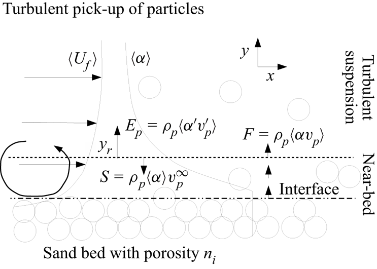
Figure 1. Definition sketch of pick-up flux  $E_p$, settling flux $S$, and total particle flux $F$.
$F$.
Winterwerp et al. (Reference Winterwerp, Bakker, Mastbergen and van Rossum1992) executed experiments with hyper-concentrated flows over an erodible bed ( $\theta >1.0$). They observed a significant deviation from the scaling relation (1.5). Based on their data, they proposed a scaling law $E_p\propto \theta ^{0.5}$. The deviations were attributed to the high near-bed concentrations that are absent in the experiments of Van Rijn (Reference Van Rijn1984). Bisschop (Reference Bisschop2018) conducted experiments at extremely high Shields parameters, up to $\theta =329$, and high near-bed concentrations. Recently, van Rijn, Bisschop & van Rhee (Reference van Rijn, Bisschop and van Rhee2019) performed a re-analysis of these data and proposed a correction of scaling (1.5) by setting $f_D={1}/{\theta }$ for $\theta >1$. According to van Rijn et al. (Reference van Rijn, Bisschop and van Rhee2019), this factor takes three processes into account that are relevant for the high Shields range: damping of turbulence in the near-bed region where the solid concentrations are extremely high, the increase of the mixture kinematic viscosity, and the increase of apparent shear resistance as a result of dilatancy of the sand bed near the interface. Van Rhee (Reference Van Rhee2010) demonstrated that this dilatancy effect can become important for a large ratio between the erosion velocity and the hydraulic conductivity of the bed, $v_e/k \gg 1$, in combination with densely packed beds (low porosity $n_i$).
To elucidate the key difference in the observations, it is helpful to reconsider the studies mentioned above in more detail. First, the erosion experiments of Van Rijn (Reference Van Rijn1984), Okayasu, Fujii & Isobe (Reference Okayasu, Fujii and Isobe2010), Cheng & Emadzadeh (Reference Cheng and Emadzadeh2016) and Bisschop (Reference Bisschop2018) cover a wide range of flow conditions, sediment sizes and measurement techniques (table 1). Van Rijn (Reference Van Rijn1984) and Cheng & Emadzadeh (Reference Cheng and Emadzadeh2016) used sediment lifts to keep the bed aligned with the floor of the flumes. The equilibrium speed of the lifts can be interpreted as the erosion velocity  $v_e$, defined in (1.2). Okayasu et al. (Reference Okayasu, Fujii and Isobe2010) constructed a flume with two sections. In the first section, particles were fixed to the flume floor, and in the second section, a sand bed could freely erode. The position of the bed was tracked near the starting point of the erodible section with a laser pointer. The bed shear stress was derived from velocity measurements in the first section and the application of standard boundary layer theory for rough walls. Bisschop (Reference Bisschop2018) used a closed-circuit flume where the flow velocity can be increased up to $10\ {\rm m}\ {\rm s}^{-1}$. The position of the bed was measured at approximately 3 m from the starting point of the erodible section using a set of conductivity probes mounted in the side wall of the flume and high-speed camera images. The conductivity probes were calibrated to obtain the absolute concentration profiles above the bed. The shear stress was estimated by measuring the pressure difference over the erodible section (over a length $\approx$6 m), which was corrected for acceleration effects and the wall shear stress contributions from the side and top walls of the flume.
Table 1. Parameter ranges in the erosion experiments ( $d_{50}$, $v_p^\infty$, $u_*$), corresponding dimensionless numbers ( $\theta$, $D_*$), entry flow at erosion measurement section being either clear-water flow (CWF) or hyper-concentrated flow (HCF), and typical concentrations in the near-bed region $\alpha _r$.
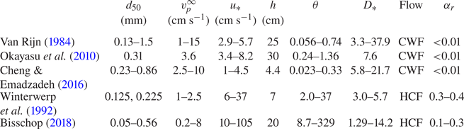
Figure 2 shows the normalized pick-up flux versus the Shields parameter of all the experimental studies mentioned above. It is seen that the scaling at relatively low Shields values differs markedly from the high near-bed concentration regimes addressed by Winterwerp et al. (Reference Winterwerp, Bakker, Mastbergen and van Rossum1992) and Bisschop (Reference Bisschop2018). Hence it is useful to distinguish clear-water flow (CWF) and hyper-concentrated flow (HCF), with a maximum near-bed concentration <0.01 and much larger than 0.01, respectively. The normalization of the pick-up flux as suggested by Einstein (Reference Einstein1950),  $\phi =E_p/\rho _p\sqrt {gd_p\varDelta }$, does not collapse all the data onto a single master curve $f(\theta )$. For Shields parameters lower than unity, a power-law trend with exponent 1.5 seems acceptable even though not perfect. In the HCF case, a power law with exponent 0.5 better describes the experimental trend. The fact that (i) the data do not collapse perfectly on master curves, and (ii) the power law exhibits an abrupt modification between CWF and HCF cases, indicates that some physical processes are not captured by the scaling law $\phi =f(\theta )$, and that further analysis is needed to explain and understand the pick-up flux. This work addresses the observed scaling behaviour of the pick-up flux from the perspective of the turbulent kinetic energy (TKE) budgets of the particle phase and the fluid phase. The main focus is to explain the striking difference in the scaling of the pick-flux in the CWF and HCF regimes by expected changes in the relative contributions of various turbulence modulation terms in the TKE equations. To analyse the CWF case, we model the fluid–particle system as a stratified single-phase flow under the Boussinesq approximation. The HCF case is analysed by using the phase-averaged TKE equations for fluid–particle systems. New scaling laws are retrieved from this analysis, which are compared with existing experimental data.
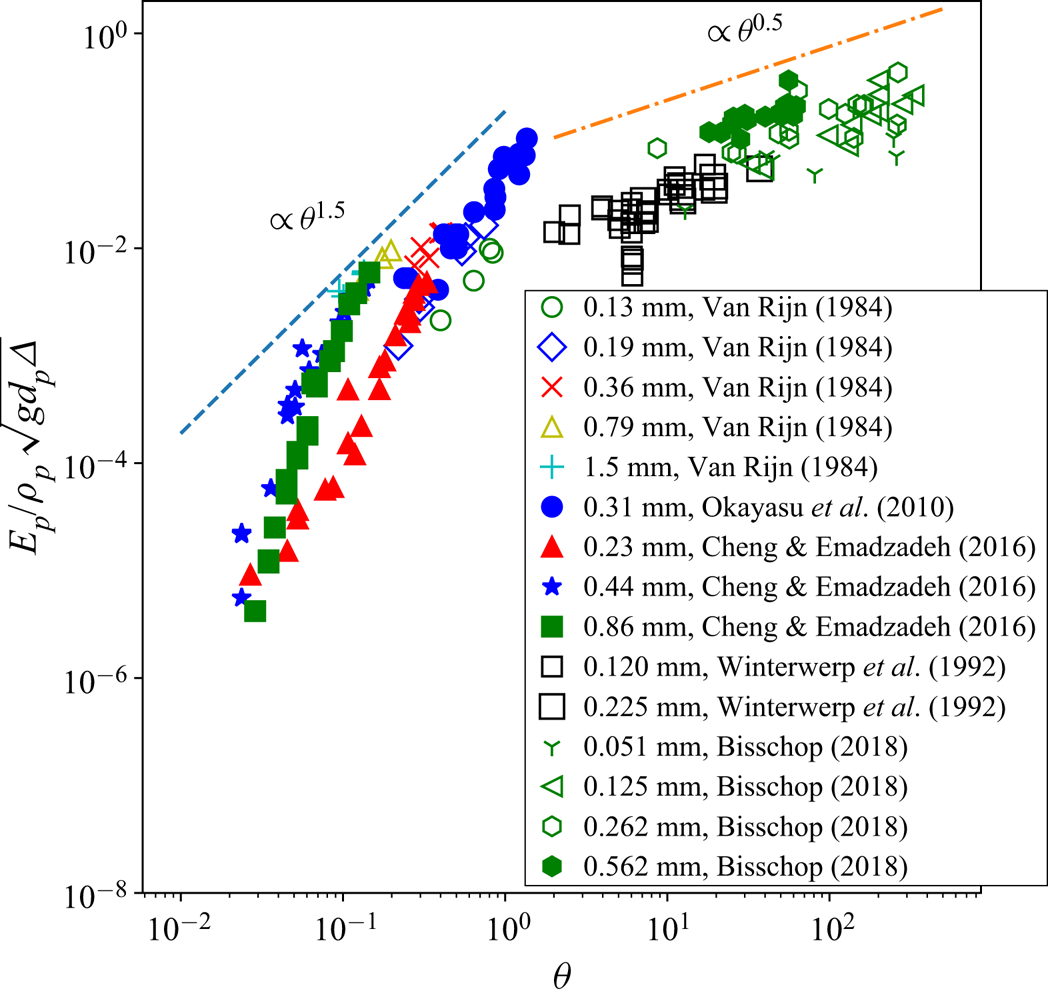
Figure 2. Scaling anomaly in the normalized pick-up flux and Shields number between CWF and HCF cases. CWF experiments: Van Rijn (Reference Van Rijn1984), Okayasu et al. (Reference Okayasu, Fujii and Isobe2010) and Cheng & Emadzadeh (Reference Cheng and Emadzadeh2016). HCF experiments: Winterwerp et al. (Reference Winterwerp, Bakker, Mastbergen and van Rossum1992) and Bisschop (Reference Bisschop2018).
2. Analysis of CWF experiments at moderate Shields numbers
For the experimental cases with CWF over erodible beds at moderate Shields numbers  $0.15<\theta <1$, the near-bed concentration is relatively low. The Stokes number in the near-bed region can be defined as $St=t_p/t_f$, with a fluid time scale $t_f=\kappa y_{r}/u_*$, that is, the ratio between the characteristic length scale of eddies in the near-bed region and the friction velocity, with $\kappa$ representing the von Kármán constant, and $t_p$ the particle drag time scale; see Appendix A. A basic estimate for $t_p$ can be obtained by considering the terminal settling velocity of a single particle in stagnant water $v_p^\infty$ (Greimann & Holly Reference Greimann and Holly2001):
 \begin{equation} t_p=\frac{v_p^\infty \rho_p}{|g|\,(\rho_p-\rho_f)}. \end{equation}
Using this estimate, we found that for the CWF experiments, the Stokes number is typically smaller than 1 for  $y_{r}>2d_p$. This implies that the relative velocity between the phases is negligible, and it suffices to consider a single-phase formulation. Because the concentrations are low, the Boussinesq approximation holds.This means that the effect of density differences can be modelled by source terms that appear on the right-hand sides of the momentum and TKE equations, while the density in the inertia terms is considered to be constant. For more details, see Appendix A.
To study the effect of self-stratification, three local characteristic numbers need to be examined: the flux Richardson number, buoyancy Froude number and buoyancy Reynolds number. First, the local flux Richardson number (Turner Reference Turner1979) is defined as the ratio between the buoyancy destruction and the shear production of TKE:
 \begin{equation} Ri_f(y)={-}\frac{|g|\,\langle{v^\prime \rho^\prime}\rangle }{\rho_0\, \langle{u^\prime v^\prime}\rangle\,\partial {\left\langle u \right\rangle}/\partial y}={-}\frac{\varDelta\,|g|\,\langle{v^\prime \alpha^\prime}\rangle }{\langle{u^\prime v^\prime}\rangle\,\partial \left\langle u \right\rangle/\partial y}, \end{equation}
where  $\left \langle u \right \rangle$ is the mean horizontal velocity, $u'$ and $v'$ are the velocity fluctuations in the horizontal and vertical directions, respectively, $\rho '$ is the density fluctuation of the mixture, $\alpha '$ is the fluctuation of the particle phase fraction, and $\rho _0\approx \rho _f$ in the dilute limit.
The gradient of the mean velocity can be modelled by the Monin–Obukhov similarity theory (Monin & Obukhov Reference Monin and Obukhov1954)
 \begin{equation} \frac{\partial \langle u\rangle}{\partial y}=\frac{u_*}{\kappa y}\,\psi_m(\zeta), \end{equation}
where  $\zeta =y/L$ is the non-dimensional height above the bed, $L$ is the Obukhov length (Obukhov Reference Obukhov1946)
 \begin{equation} L=\frac{u_*^3}{\varDelta\,|g| \left\langle v'\alpha' \right\rangle\kappa}, \end{equation}
and  $\psi _m$ is the stability function for the momentum flux. The Obukhov length is a profile-dependent parameter that characterizes the strength of the stratification. It represents the theoretical height where $Ri_f=1$ based on a neutrally stratified $\psi _m=1$ velocity profile. Substitution of (2.3) in (2.2) gives
 \begin{equation} Ri_f(\zeta)=\frac{\varDelta\,|g|\,\langle v'\alpha'\rangle\,\kappa y}{u_*^3\,\psi_m({\zeta})}=\frac{\zeta}{\psi_m(\zeta)}. \end{equation}
The second control parameter is the buoyancy Froude number (Lesieur Reference Lesieur1990)
 \begin{equation} \displaystyle Fr=\left(\frac{l_B}{l_e}\right)^{2/3}, \end{equation}
where  $l_e=u_*^3/\varepsilon$ is a turbulent flow scale associated with the most energetic eddies in the boundary layer at height $y$, and $l_B=(\varepsilon /N^3)^{1/2}$ is the Osmidov length scale (Osmidov Reference Osmidov1975), with $\varepsilon =u_*^3\,\psi _m(\zeta )/\kappa y$ the turbulent dissipation, and $N$ the Brunt–Vaïsala frequency (Turner Reference Turner1979; Lesieur Reference Lesieur1990) given by
 \begin{equation} \displaystyle N^2={-} \frac{|g|}{{\rho_0}}\,\frac{{\rm d} \langle\rho\rangle}{{{\rm d} y}}. \end{equation}
Parameter  $N$ is also known as the buoyancy frequency, which is the frequency of an internal wave in a stably stratified fluid. The Osmidov scale $l_B$ is a local scale for the stratification, and it represents the maximum eddy length scale that can develop in the presence of internal waves such that the turnover time of the eddies at that scale equals $1/N$.
The density profile  $\left \langle \rho \right \rangle =\left \langle \alpha \right \rangle \rho _p + (1-\left \langle \alpha \right \rangle )\, \rho _f$ is a function of the local phase fraction such that
 \begin{equation} \displaystyle \frac{{\rm d} \langle\rho\rangle}{{\rm d} y} = \rho_f \varDelta\,\frac{{\rm d} \langle\alpha\rangle}{{{\rm d} y}}. \end{equation}
The gradient of the phase fraction can also be described by the Monin–Obukhov similarity theory:
 \begin{equation} \frac{\partial \langle\alpha\rangle}{\partial y}=\frac{\langle{v'\alpha'}\rangle}{u_*}\,\frac{\psi_\alpha(\zeta)}{\kappa y}, \end{equation}
where  $\psi _\alpha$ is the stability function for $\alpha$. Since for the clear-water case $\rho _0\approx \rho _f$, it follows that
 \begin{equation} N^2=\frac{|g|\,\varDelta\,\langle{v'\alpha'}\rangle\,\psi_\alpha(\zeta)}{\kappa y u_*}. \end{equation}
This implies that the local buoyancy Froude number and local flux Richardson number can be related by
 \begin{equation} Fr=\frac{1}{\sqrt{Ri_f}}\,\sqrt{\frac{\psi_m}{\psi_\alpha}}, \end{equation}
where it is expected that  $\psi _m\approx \psi _\alpha$. This signifies that self-stratification in the near bed region can be interpreted in terms of both buoyancy destruction of TKE and stability constraints imposed by internal waves associated with the vertical density gradient above the bed.
The third control parameter of stratified flows is the buoyancy Reynolds number (Venayagamoorthy & Koseff Reference Venayagamoorthy and Koseff2016) defined as
 \begin{equation} Re_b=\frac{\varepsilon}{\nu_f N^2}. \end{equation}
The buoyancy Reynolds number can be related to the ratio of the Osmidov length scale  $l_B$ and the Kolmogorov length scale $l_\eta =(\nu _f^3/\varepsilon )^{1/4}$ since $l_B/l_\eta =Re_b^{3/4}$. If the separation between these scales is too small, then the turbulent cascade cannot develop, which in turn drives the flow towards a laminar state and reduces particle entrainment. Figure 3 illustrates this argument. Using (2.12), $\varepsilon =u_*^3\,\psi _m(\zeta )/\kappa y$ and (2.10), it follows that
 \begin{equation} Re_b=\frac{Re_{\tau}(y)}{Ri_f(y)}\,\frac{\kappa}{\psi_{\alpha}(\zeta) }, \end{equation}
where  $Re_{\tau }=u_* y/\nu _f$ is the friction Reynolds number. In the regime of minimum scale separation between $l_B$ and $l_\eta$, $Re_b$ reaches a critical value, and according to (2.13), this will impose a constraint on the local flux Richardson number $Ri_f^c\propto Re_\tau \kappa /\psi _\alpha$. By virtue of (2.5), the definition of the pick-up flux, $\phi =\langle {v'\alpha '}\rangle /\sqrt {\varDelta g d_p}$ and $\psi _\alpha \approx \psi _m$, for small $\zeta$, it then follows that
 \begin{equation} \phi\propto\lim_{\zeta \to 0}\frac{\psi_m(\zeta)}{\psi_\alpha(\zeta)}\,Re_p\,\theta^{1.5}=Re_p\,\theta^{1.5}, \end{equation}
where  $Re_p=d_pu_*/\nu _f$ is the particle Reynolds number based on the friction velocity.
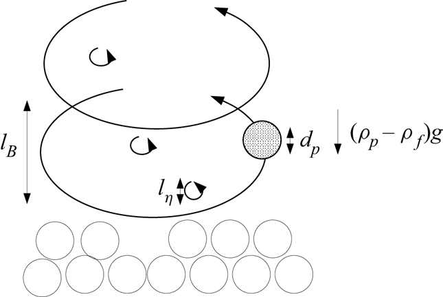
Figure 3. Constraint on the ratio between the Osmidov length scale  $l_B$ and the Kolmogorov scale $l_\eta$. Increasing the pick-up flux results in a reduction of $l_B$ by buoyancy until a critical value $l_B/l_\eta$ (i.e. $Re_b$) is reached. This argument corresponds to scaling (2.14).
In dilute suspensions, the inter-particle distance allows enough space for TKE dissipation events to evolve, as in CWF. However, it is possible that a finite-size effect sets in when  $l_B\approx d_p$: the energy carrying eddies might no longer be able to induce a net lift or drag force on the particles at the interface, at least not in a statistical-averaged sense; see figure 4. From this constraint on the Osmidov length scale and (2.13), it follows that
 \begin{equation} Ri_f^c\propto \left(\frac{\kappa y_r}{d_p} \right)^{4/3}\frac{1}{\psi_\alpha\psi_m^{1/3}}, \end{equation}
and for the non-dimensional pick-up flux at small  $\zeta$,
 \begin{equation} \phi\propto \frac{\psi_m^{2/3}}{\psi_\alpha}\left(\frac{\kappa y_r}{d_p} \right)^{1/3}\theta^{1.5}\approx \left(\frac{\kappa y_r}{d_p} \right)^{1/3}\theta^{1.5}. \end{equation}
This leaves a weak dependence on the choice of the reference height.
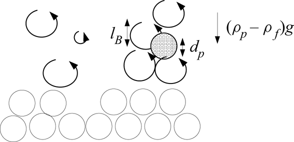
Figure 4. Constraint on the ratio between the Osmidov length scale  $l_B$ and the particle size $d_p$. Increasing the pick-up flux results in a reduction of $l_B$ by buoyancy until a critical value $l_B/d_p$ is reached. This line of reasoning results in scaling (2.16).
In conclusion, in the CWF experiments at moderate Shields numbers  $0.15<\theta <1.0$, by a self-stratification argument, two scaling laws can be expected, (2.14) and (2.16) for sub-Kolmogorov and finite-size particles, respectively. We will test the scaling relations, as well as the empirical relation given by (1.5), in § 4. Note that they all have the same $\theta ^{1.5}$ proportionality, but differ in the pre-factor in front of this term, notably the dependence on the particle diameter $d_p$.
3. Analysis of HCF experiments at high Shields numbers
For HCF over erodible beds at high Shields numbers, it is required to address more generic equations for the TKE of dispersed multi-phase flows.
These equations appeared in various forms in literature. In this work, we use the framework of Fox (Reference Fox2014) and adopt the same notations here for convenience. The two-fluid model of Fox (Reference Fox2014) is restricted to drag forces only, but we think that this is not a limitation for this study. Although the Saffman lift force is important for the pick-up of individual particles from the bed (see § 1), we assume that it is sufficient to restrict our near-bed flow analysis to the drag force. Jha & Bombardelli (Reference Jha and Bombardelli2010) demonstrated that adding the lift force in a two-fluid model for particle-laden channel flows modifies the flow dynamics only marginally.
To study the departures from stratified single-phase flow under the Boussinesq approximation, it is helpful to combine the balances for the TKE of the fluid and particle phases. In the equations for the fluid and particle TKE as derived by Fox (Reference Fox2014), the buoyancy term, as it appears under the Boussinesq approximation, is difficult to recognize. In Appendix A, it is shown that after multiple manipulations of the equations of Fox (Reference Fox2014), the combined TKE balance of the two phases can be written as follows:
 \begin{align} &\underbrace{\frac{\partial\rho_f\left\langle 1-\alpha
\right\rangle k_f+\rho_p\left\langle \alpha \right\rangle
k_p}{\partial t}}_{\textit{time change}}
+\boldsymbol{\nabla}\boldsymbol{\cdot}\biggl[\underbrace{\rho_f\left\langle
1-\alpha \right\rangle\left\langle \boldsymbol{u}_f
\right\rangle_fk_f+ \rho_f\left\langle 1-\alpha
\right\rangle\frac{1}{2}\left\langle
\boldsymbol{u}_f'''\boldsymbol{u}_f'''\boldsymbol{\cdot}\boldsymbol{u}_f'''
\right\rangle_f}_{\textit{transport by mean fluid velocity
and fluid velocity fluctuations}} \nonumber\\ &\quad +\underbrace{ {\left\langle 1-\alpha
\right\rangle}\left\langle p_f'\boldsymbol{u}_f'''
\right\rangle_f-\left\langle
\boldsymbol{\sigma}_f\boldsymbol{\cdot}\boldsymbol{u}_f'''
\right\rangle}_{ \textit{transport by fluid stresses}} \nonumber\\ &\quad +\underbrace{\rho_p\left\langle \alpha
\right\rangle\left\langle \boldsymbol{u}_p \right\rangle_p
k_p+\rho_p\left\langle \alpha
\right\rangle\frac{1}{2}\left\langle
\boldsymbol{u}_p''\boldsymbol{u}_p''\boldsymbol{\cdot}
\boldsymbol{u}_p'' \right\rangle_p}_{\textit{transport by
mean particle velocity and particle velocity
fluctuations}} \nonumber\\ &\quad +\underbrace{\left\langle
\alpha \right\rangle\left\langle p_f'\boldsymbol{u}_p''
\right\rangle_p+\rho_p\left\langle \alpha
\right\rangle\left\langle \boldsymbol{\mathsf{P}}_p
\boldsymbol{\cdot} \boldsymbol{u}_p''
\right\rangle_p\biggr]}_{\textit{transport by fluid pressure
fluctuations and particle stresses}} \nonumber\\ &\quad =\underbrace{-\rho_f\left\langle 1-\alpha
\right\rangle\left\langle
\boldsymbol{u}_f'''\boldsymbol{u}_f''' \right\rangle_f:
\boldsymbol{\nabla}\left\langle \boldsymbol{u}_f
\right\rangle_f-\rho_p\left\langle \alpha
\right\rangle\left\langle
\boldsymbol{u}_p''\boldsymbol{u}_p''
\right\rangle_p:\boldsymbol{\nabla}\left\langle
\boldsymbol{u}_p \right\rangle_p}_{\textit{shear production
in both phases, conversion MKE-TKE}} \nonumber\\ &\qquad +\underbrace{\left\langle
p_f'\boldsymbol{\nabla}\boldsymbol{\cdot}\alpha'\left(\left\langle
\boldsymbol{u}_f \right\rangle_f- \left\langle
\boldsymbol{u}_p \right\rangle_p\right)
\right\rangle}_{\textit{compression effect, conversion
MKE-TKE}} \nonumber\\ &\qquad
+\underbrace{\frac{\rho_p\left\langle \alpha
\right\rangle}{ t_p}\,\frac{\left\langle
\alpha'\boldsymbol{u}_f' \right\rangle}{\left\langle \alpha
\right\rangle\left\langle 1- \alpha
\right\rangle}\boldsymbol{\cdot}\left(\left\langle
\boldsymbol{u}_p \right\rangle_p-\left\langle
\boldsymbol{u}_f \right\rangle_f-\frac{\left\langle
\alpha'\boldsymbol{u}_f' \right\rangle}{\left\langle \alpha
\right\rangle\left\langle 1-\alpha
\right\rangle}\right)}_{\textit{drag conversion MKE-TKE,
contains buoyancy via momentum equations,
see (A38)}} \nonumber\\ &\qquad
\underbrace{-\left\langle \boldsymbol{\nabla}
\boldsymbol{u}_f''':\boldsymbol{\sigma}_f
\right\rangle}_{\textit{viscous dissipation, conversion
TKE-heat}}+\underbrace{\rho_p\left\langle \alpha
\right\rangle\left\langle \boldsymbol{\mathsf{P}}_p:
\boldsymbol{\nabla} \boldsymbol{u}_p''
\right\rangle_p}_{\textit{conversion TKE-$\varTheta_p$}}\nonumber\\ &\qquad - \underbrace{\frac{\rho_p\left\langle \alpha \right\rangle}{
t_p}\left\langle
\left|\boldsymbol{u}_f''-\boldsymbol{u}_p''\right|^2
\right\rangle_p}_{ \textit{drag dissipation, conversion
TKE-heat}},
\end{align}
\begin{align} &\underbrace{\frac{\partial\rho_f\left\langle 1-\alpha
\right\rangle k_f+\rho_p\left\langle \alpha \right\rangle
k_p}{\partial t}}_{\textit{time change}}
+\boldsymbol{\nabla}\boldsymbol{\cdot}\biggl[\underbrace{\rho_f\left\langle
1-\alpha \right\rangle\left\langle \boldsymbol{u}_f
\right\rangle_fk_f+ \rho_f\left\langle 1-\alpha
\right\rangle\frac{1}{2}\left\langle
\boldsymbol{u}_f'''\boldsymbol{u}_f'''\boldsymbol{\cdot}\boldsymbol{u}_f'''
\right\rangle_f}_{\textit{transport by mean fluid velocity
and fluid velocity fluctuations}} \nonumber\\ &\quad +\underbrace{ {\left\langle 1-\alpha
\right\rangle}\left\langle p_f'\boldsymbol{u}_f'''
\right\rangle_f-\left\langle
\boldsymbol{\sigma}_f\boldsymbol{\cdot}\boldsymbol{u}_f'''
\right\rangle}_{ \textit{transport by fluid stresses}} \nonumber\\ &\quad +\underbrace{\rho_p\left\langle \alpha
\right\rangle\left\langle \boldsymbol{u}_p \right\rangle_p
k_p+\rho_p\left\langle \alpha
\right\rangle\frac{1}{2}\left\langle
\boldsymbol{u}_p''\boldsymbol{u}_p''\boldsymbol{\cdot}
\boldsymbol{u}_p'' \right\rangle_p}_{\textit{transport by
mean particle velocity and particle velocity
fluctuations}} \nonumber\\ &\quad +\underbrace{\left\langle
\alpha \right\rangle\left\langle p_f'\boldsymbol{u}_p''
\right\rangle_p+\rho_p\left\langle \alpha
\right\rangle\left\langle \boldsymbol{\mathsf{P}}_p
\boldsymbol{\cdot} \boldsymbol{u}_p''
\right\rangle_p\biggr]}_{\textit{transport by fluid pressure
fluctuations and particle stresses}} \nonumber\\ &\quad =\underbrace{-\rho_f\left\langle 1-\alpha
\right\rangle\left\langle
\boldsymbol{u}_f'''\boldsymbol{u}_f''' \right\rangle_f:
\boldsymbol{\nabla}\left\langle \boldsymbol{u}_f
\right\rangle_f-\rho_p\left\langle \alpha
\right\rangle\left\langle
\boldsymbol{u}_p''\boldsymbol{u}_p''
\right\rangle_p:\boldsymbol{\nabla}\left\langle
\boldsymbol{u}_p \right\rangle_p}_{\textit{shear production
in both phases, conversion MKE-TKE}} \nonumber\\ &\qquad +\underbrace{\left\langle
p_f'\boldsymbol{\nabla}\boldsymbol{\cdot}\alpha'\left(\left\langle
\boldsymbol{u}_f \right\rangle_f- \left\langle
\boldsymbol{u}_p \right\rangle_p\right)
\right\rangle}_{\textit{compression effect, conversion
MKE-TKE}} \nonumber\\ &\qquad
+\underbrace{\frac{\rho_p\left\langle \alpha
\right\rangle}{ t_p}\,\frac{\left\langle
\alpha'\boldsymbol{u}_f' \right\rangle}{\left\langle \alpha
\right\rangle\left\langle 1- \alpha
\right\rangle}\boldsymbol{\cdot}\left(\left\langle
\boldsymbol{u}_p \right\rangle_p-\left\langle
\boldsymbol{u}_f \right\rangle_f-\frac{\left\langle
\alpha'\boldsymbol{u}_f' \right\rangle}{\left\langle \alpha
\right\rangle\left\langle 1-\alpha
\right\rangle}\right)}_{\textit{drag conversion MKE-TKE,
contains buoyancy via momentum equations,
see (A38)}} \nonumber\\ &\qquad
\underbrace{-\left\langle \boldsymbol{\nabla}
\boldsymbol{u}_f''':\boldsymbol{\sigma}_f
\right\rangle}_{\textit{viscous dissipation, conversion
TKE-heat}}+\underbrace{\rho_p\left\langle \alpha
\right\rangle\left\langle \boldsymbol{\mathsf{P}}_p:
\boldsymbol{\nabla} \boldsymbol{u}_p''
\right\rangle_p}_{\textit{conversion TKE-$\varTheta_p$}}\nonumber\\ &\qquad - \underbrace{\frac{\rho_p\left\langle \alpha \right\rangle}{
t_p}\left\langle
\left|\boldsymbol{u}_f''-\boldsymbol{u}_p''\right|^2
\right\rangle_p}_{ \textit{drag dissipation, conversion
TKE-heat}},
\end{align}
where  $k_f$ and $k_p$ are the TKE, in kinematic units, of the fluid and particle phases, respectively, $\boldsymbol {u}_f$ and $\boldsymbol {u}_p$ are the velocities of each phase, $\left \langle \cdot \right \rangle$ represents standard Reynolds averaging, $\left \langle \cdot \right \rangle _f$ and $\left \langle \cdot \right \rangle _p$ are conditional averages over each phase, $A'$,
$A'$,  $A''$ and $A'''$ denote fluctuations with respect to the Reynolds average, particle phase average and fluid phase average, respectively, $\boldsymbol{\mathsf{P}}_p$ is the particle stress, $\boldsymbol {\sigma }_f$ is the viscous stress, $p_f$ is the fluid pressure, and $t_p$ is a constant time scale associated with drag.
The left hand-side of (3.1) contains the time change of TKE and transport of TKE by the mean flows, turbulent fluctuations, pressure fluctuations, collisional stress and viscous stress. Similar transport terms appear in the TKE equation for stratified single-phase flow.
The first two terms on the right-hand side of (3.1) represent the shear production of the fluid and particle phases. Similar to single-phase flow, they describe the transfer from kinetic energy of the mean flow (or mean kinetic energy, MKE) to TKE. The next two terms describe the transfer from MKE to TKE by pressure coupling and drag forces. Using the momentum balances of the fluid and particle phases, the drag contribution can be related to the buoyancy term as it appears in the TKE equation under the Boussinesq approximation; see (A5) in Appendix A. The last three terms describe the conversion from TKE into heat and granular temperature. After the conversion into granular temperature, energy can be further converted into heat by drag and inelastic collisions; see Fox (Reference Fox2014). Figure 5 gives an overview of the energy flows between the different variables. In the context of this study, the relation between the conversion of MKE to TKE by the mean shear, the conversion of TKE to MKE via drag, and the conversion of MKE to potential energy (PE) is important. For increasing particle concentrations, granular dissipation  $\epsilon _p$, and drag dissipation become more relevant, next to the viscous dissipation of TKE $\epsilon _f$.
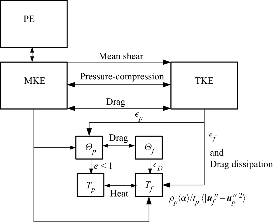
Figure 5. Energy flows between PE, MKE, TKE, granular temperature  $\varTheta _p$, temperature of the particles $T_p$, pseudo-TKE $\varTheta _f$ (turbulence in the wake of the particles) and temperature of the fluid $T_f$, where $e$ is the coefficient of restitution between the particles, $\epsilon _f$ is the viscous dissipation of fluid TKE, $\epsilon _p$ is the granular dissipation of particle TKE, and $\epsilon _D$ is the small-scale viscous dissipation associated with pseudo-turbulence (Fox Reference Fox2014).
Now the TKE budget is written in a convenient form to study the departures from the Boussinesq approximation, there is an opening to retrieve possible scaling laws for the pick-up flux in the HCF regime at high Shields numbers. In the previous section, it is anticipated that the pick-up flux at moderate Shields numbers and low near-bed concentrations is controlled by the balance between the shear production, viscous dissipation and buoyancy destruction terms. For increasing near-bed concentrations and Shields numbers, the magnitude of each term in (3.1) will likely change. For simplicity, we assume that although the relative contribution of each transport term will vary in the HCF regime, the key deviations that control the pick-up flux stem from differences in the source terms on the right-hand side of (3.1).
First, we need to estimate the combined shear production of both phases. The assumption is that in the flow direction, the macroscopic particle/fluid slip velocity is small at the length scale ( $\kappa y$) of the mean flow and of the turbulent fluctuations in the energy-containing range. In then follows that $\left \langle u_p \right \rangle _p\approx \left \langle u_f \right \rangle _f$ and $\left \langle u_p''v_p'' \right \rangle _p\approx \left \langle u_f''v''_f \right \rangle _f$. The combined shear production term from both phases then becomes
 \begin{align} &-\rho_f\left\langle 1-\alpha \right\rangle\left\langle u_f'''v_f''' \right\rangle_f\frac{\partial \left\langle u_f \right\rangle_f}{\partial y}-\rho_p\left\langle \alpha \right\rangle\left\langle u_p''v_p'' \right\rangle_p\frac{\partial \left\langle u_p \right\rangle_p}{\partial y}\nonumber\\ &\quad \approx \rho_m\left\langle u_f'''v_f''' \right\rangle_f\frac{\partial \left\langle u_f \right\rangle_f}{\partial y}. \end{align}
Next, we estimate the turbulent shear stress by
 \begin{equation} -\rho_m\left\langle u_f'''v_f''' \right\rangle_f={-}\rho_m\left\langle u_f'v_f' \right\rangle_f\approx \rho_m u_*^2, \end{equation}
which is expected to hold in the logarithmic (or constant-stress) layer as long as the Reynolds number is sufficiently high. Furthermore, assuming that the fluid velocity profile obeys the standard logarithmic scaling as in single-phase flow, the velocity gradient becomes equal to
 \begin{equation} \frac{\partial \left\langle u_f \right\rangle_f}{\partial y}\approx \frac{u_*}{\kappa y}. \end{equation}
The validity of the logarithmic scaling for the HCF regime has been confirmed by velocity measurements by Winterwerp et al. (Reference Winterwerp, de Groot, Mastbergen and Verwoert1990) and Bisschop (Reference Bisschop2018). Our final estimate of the shear production term becomes
 \begin{equation} -\rho_f\left\langle 1-\alpha \right\rangle\left\langle u_f'''v_f''' \right\rangle_f\frac{\partial \left\langle u_f \right\rangle_f}{\partial y}-\rho_p\left\langle \alpha \right\rangle\left\langle u_p''v_p'' \right\rangle_p\frac{\partial \left\langle u_p \right\rangle_p}{\partial y}\approx \rho_m\frac{u_*^3}{\kappa y}, \end{equation}
with  $\rho _m=\rho _f+(\rho _p-\rho _f)\left \langle \alpha \right \rangle$; for sediment-water flows, it typically holds that $\rho _p=2.6\rho _f$ so $\rho _m=\rho _f(1+1.6\left \langle \alpha \right \rangle )$. The shear production is balanced by the other terms: viscous dissipation, transfer to granular temperature, conversion of MKE to TKE, modified buoyancy destruction and drag dissipation. We expect that in the HCF regime, the transfer to granular temperature and drag dissipation will start to consume the largest portion of the TKE production, while changes in the MKE–TKE conversion have secondary effects.
From this conjecture, let us try to find some estimates for the pick-up flux in the HCF regime. The transfer to granular temperature term can be decomposed in two parts:
 \begin{equation} {\rho_p\left\langle \alpha \right\rangle\left\langle \boldsymbol{\mathsf{P}}_p:\boldsymbol{\nabla} \boldsymbol{u}_p'' \right\rangle_p}=\left\langle p_p\boldsymbol{\nabla}\boldsymbol{\cdot} \boldsymbol{u}_p'' \right\rangle-\left\langle \boldsymbol{\sigma}_p:\boldsymbol{\nabla}\boldsymbol{u}_p'' \right\rangle, \end{equation}
where  $p_p$ is the particle pressure, and $\boldsymbol{\sigma} _p$ is the particle shear stress. The pressure dilatation term in (3.6) can be modelled as
 \begin{equation} \left\langle p_p\,\boldsymbol{\nabla}\boldsymbol{\cdot}\boldsymbol{u}_p'' \right\rangle=\left\langle [1+4\alpha\, g_0(\alpha)]\varTheta\,\boldsymbol{\nabla}\boldsymbol{\cdot}\boldsymbol{u}_p'' \right\rangle_p, \end{equation}
where  $g_0(\alpha )$ is the radial distribution function, and $\varTheta$ is the granular temperature (Fox Reference Fox2014). In the dilute case, this term is usually neglected, with the argument that $\varTheta$ varies over the integral length scales and thus does not correlate with gradients of velocity fluctuations that live on a smaller scale. It is expected that a diverging flow field $\boldsymbol {u}_p''$ is associated with a lower concentration ( $\alpha '<0$). As a result, the dilation term is likely negative at high particle concentrations. The second term on the right-hand side of (3.6) can be recognized as the dissipation rate of particle TKE by the particle shear stress. Combining the effect of pressure dilatation and shear provides the following definition of the dissipation rate of particle TKE:
 \begin{equation} \left\langle \boldsymbol{\sigma}_p:\boldsymbol{\nabla} \boldsymbol{u}_p'' \right\rangle-\left\langle p_p\boldsymbol{\nabla}\boldsymbol{\cdot}\boldsymbol{u}_p'' \right\rangle=\left\langle \alpha \right\rangle\rho_p{\epsilon}_p, \end{equation}
where it should be noted that this dissipation term is not a direct conversion into heat, but the particle TKE first converts into granular temperature and then converts into heat by particle collisions and particle–fluid drag on the level of individual granular fluctuations. On the other hand, the drag dissipation term on the right-hand side of (3.1) is a direct conversion into heat by particle–fluid drag; see figure 5.
To estimate the relative contribution of the drag dissipation and  $\epsilon _p$, it is helpful to consider the viscous time scale $t_\eta$, the particle-drag time scale $t_p$ and the turnover time of the most energetic eddies in the near-bed region $t_e=\kappa y/u_*$. The viscous time scale can be estimated as
 \begin{equation} t_\eta=\left(\frac{\mu_{m}}{\rho_m \epsilon_m}\right)^{1/2}, \end{equation}
where the subscript  $m$ indicates variables defined for the particle–fluid mixture. Typically, the effective shear viscosity of the mixture can be modelled as $\mu _m=\mu _f(1-{\left \langle \alpha \right \rangle }/{\left \langle \alpha \right \rangle _m})^{-2}$ (Maron & Pierce Reference Maron and Pierce1956; Guazzelli & Pouliquen Reference Guazzelli and Pouliquen2018), with $\left \langle \alpha \right \rangle _m\approx 0.6$ the maximum flowable packing fraction. Using $\epsilon _m=u_*^3/\kappa y$ and $\rho _m=\rho _f(1+\varDelta \left \langle \alpha \right \rangle )$, it follows that
 \begin{equation} t_{\eta}=\left(\frac{\left(1-\dfrac{\left\langle \alpha \right\rangle}{\left\langle \alpha \right\rangle_m}\right)^{{-}2}}{1+\varDelta\left\langle \alpha \right\rangle}\right)^{1/2}\frac{\kappa y}{u_*}\,\frac{1}{\sqrt{\kappa \,Re_\tau}}. \end{equation}
Now if  $t_{\eta }< t_p< t_e$, then it can be anticipated that the turbulent cascade breaks down at the time scale $t_p$, and drag dissipation is the most important dissipation mechanism. If $t_p< t_\eta < t_{e}$, then the turbulent cascade is halted by viscous dissipation, and at high particle concentrations it is expected that $\epsilon _p$ is at least of the same order as $\epsilon _f$ or higher (higher for higher concentration). By using (3.10), the constraint $t_\eta < t_p$ can be written as
 \begin{equation} \left(\frac{\left(1-\dfrac{\left\langle \alpha \right\rangle}{\left\langle \alpha \right\rangle_m}\right)^{{-}2}}{1+ \varDelta\left\langle \alpha \right\rangle}\right)^{1/2}\frac{1}{\sqrt{\kappa \,Re_\tau}}< St, \end{equation}
which sets a lower bound on the Stokes number, and likewise the constraint  $t_p< t_\eta$ sets an upper bound on the Stokes number. This implies that the Stokes number controls the relative contribution of the drag dissipation (high Stokes numbers) and $\epsilon _p$ (low Stokes numbers) in the HCF regime.
Using estimates obtained for statistically steady-state, homogeneous and isotropic turbulence (Fox Reference Fox2014), we derive in Appendix B the scaling for the dissipation of particle TKE
 \begin{equation} \epsilon_p=St\left(\frac{2}{St+2}\right)^2\frac{k_f}{t_p}, \end{equation}
and for the dissipation by drag forces,
 \begin{equation} \frac{1}{t_p}\left\langle \left|\boldsymbol{u}_f''-\boldsymbol{u}_p''\right|^2 \right\rangle_p=2\,\frac{k_f}{t_p}\left(\frac{St}{2+St}\right)^2. \end{equation}
The ratio  $R$ of (3.12) and (3.13) is
 \begin{equation} R=\frac{2}{St}, \end{equation}
which indicates that at high Stokes numbers, drag dissipation is dominant, and at low Stokes numbers, turbulent dissipation of particle TKE overcomes the drag dissipation. This is in line with estimate (3.11) obtained from the analysis of the relevant time scales.
For the flow in the near-bed region, the Stokes number can be estimated as  $St={u_*t_p}/{\kappa y}$. Estimate (3.14) then suggests that close to the bed, drag dissipation is dominant, while the importance of particle TKE dissipation increases when moving from the bed. At small $y$ and thus high Stokes numbers, $St\gg 1$, the dominant balance is between drag dissipation and shear production, yielding
 \begin{equation} \frac{\rho_p\left\langle \alpha \right\rangle}{t_p}\left\langle \left|\boldsymbol{u}_f''-\boldsymbol{u}_p''\right|^2 \right\rangle_p=2\rho_p\left\langle \alpha \right\rangle\frac{k_f}{t_p}\left(\frac{St}{2+St}\right)^2=\rho_m\,\frac{u_*^3}{\kappa y}. \end{equation}
Since  $k_f\propto u_*^2$, and using $St={u_*t_p}/{\kappa y}$, it follows that for $St\gg 1$,
 \begin{equation} \left\langle \alpha \right\rangle\propto \frac{(2+St)^2}{St}\approx St, \end{equation}
which indicates that the near-bed concentration increases with the Stokes number. At higher regions in the profile, such that  $St\ll 1$, the key balance is between dissipation of particle TKE and shear production,
 \begin{equation} \left\langle \alpha \right\rangle\rho_p\,St\left(\frac{2}{St+2}\right)^2\frac{k_f}{t_p}=\rho_m\,\frac{u_*^3}{\kappa y}. \end{equation}
This indicates that for  $St\ll 1$,
 \begin{equation} \left\langle \alpha \right\rangle\propto (St+2)^2\propto St^0. \end{equation}
From the limiting cases (3.16) and (3.18), the following scaling can be anticipated for the near-bed region:
 \begin{equation} \left\langle \alpha \right\rangle\propto St^{\xi}, \end{equation}
with  $0<\xi <1$, where the scaling exponent should be determined from concentration measurements in the near-bed region.
The following scaling of the pick-up flux is then expected:
 \begin{equation} E_p\propto \rho_p \left\langle \alpha \right\rangle u_*\propto{\rho_p}\,{St}^{\xi}\,u_*. \end{equation}
In the traditional non-dimensional form, this becomes
 \begin{equation} \phi\propto St^{\xi}\,\theta^{0.5}. \end{equation}
4. Results and discussion
In this section, we reconsider the experimental data introduced in § 1. Figure 6 shows the Obukhov length versus the Shields parameter. A minimum in the Obukhov length is observed for the CWF experiments conducted in the range  $0.15<\theta <1$. This indicates that stratification effects, as discussed in § 2, could be present in this range, but buoyancy destruction is likely negligible for the other cases.
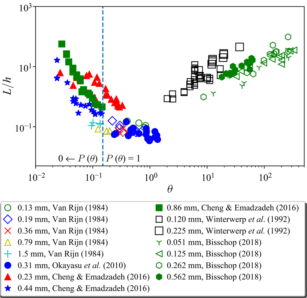
Figure 6. Obukhov length over channel height versus the Shields parameter. The dashed vertical line indicates the region ( $\theta < 0.15$) where the pick-up probability of a single grain strongly influences the pick-up rate.
In the CWF experiments with a lower Shields number,  $\theta <0.15$, particle contact load is the dominant transport form; see figure 7. For this reason, it is very unlikely that the pick-up flux for those cases is controlled by TKE budget considerations. It is more reasonable to expect that the pick-up flux in this regime is controlled by the probability that an individual particle is lifted from the bed by the turbulent flow that developed above the fixed bed section upstream of the erodible bed section in the CWF experiments.
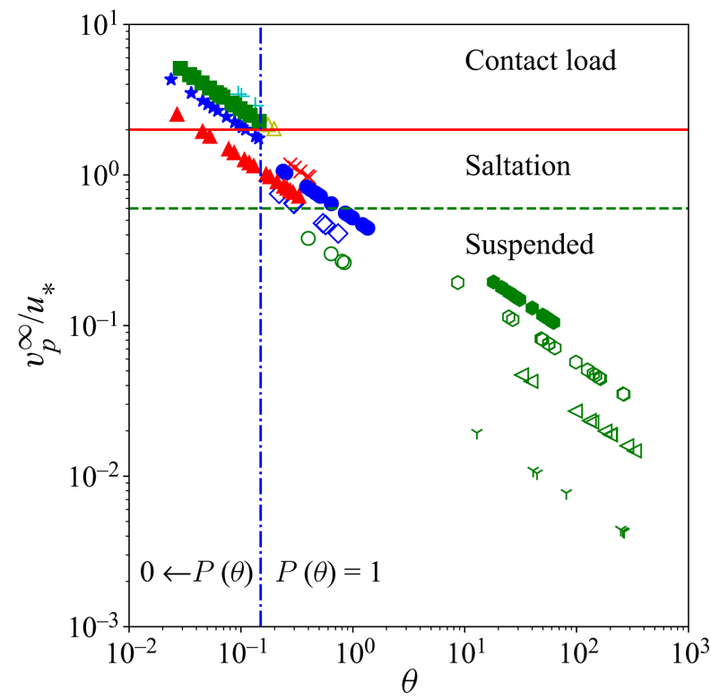
Figure 7. Ratio of the terminal settling velocity and friction velocity plotted against the Shields parameter to identify the expected transport mode. Symbols are as defined in figure 2. The horizontal lines indicate the threshold values for the different transports (Dey Reference Dey2014).
In the experiments of Bisschop (Reference Bisschop2018), where  $\theta \gg 1$, the near-bed concentration was measured by conductivity probes with vertical separation 1 cm. The first measurement point at 1 cm height above the bed shows that $\left \langle \alpha \right \rangle >0.1$ for all cases; see figure 8. In this case, the Boussinesq assumption is no longer valid. As detailed in § 3, mechanisms other than stratification are probably controlling the scaling of the pick-up flux. This is consistent with the observed high values of the Obukhov length in figure 6. It is expected that the near-bed concentration depends only weakly on the Stokes number, which could be modelled by (3.19). Figure 8 demonstrates that this type of scaling is reasonably accurate, using a simplified Stokes number $St={t_p u_*}/{\kappa y}$, with a constant $t_p$ modelled by (2.1).
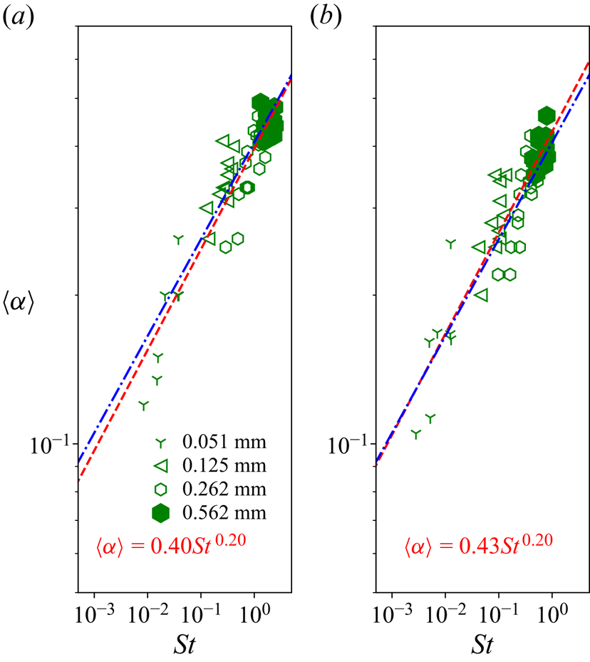
Figure 8. Near-bed concentration versus Stokes number (see (2.1)), measured at (a)  $1$ cm and (b) $3$ cm height above the bed; data of Bisschop (Reference Bisschop2018). Symbols are as defined in figure 2. The dashed line represents a least squares regression for both heights separately, $\left \langle \alpha \right \rangle =0.41\,St^{0.20}$. The dash-dotted line is a least squares regression for the combined measurements at $1$ and $3$ cm height above the bed.
Now we will examine the scaling of the pick-up flux for both the CWF and HCF experiments. Regarding the CWF experiments, figure 9 shows the two scaling laws for the dimensionless pick-up flux (2.14) and (2.16), as derived from buoyancy arguments in § 2. It is observed that (2.14) gives a reasonably accurate fit to the experimental data. This indicates that stratification effects play an important role in the pick-up flux in the CWF regime at moderate Shields numbers. The assumption that the Osmidov length scale is halted by the particle size, which leads to (2.16), could be valid in some cases. The limited quality of the scaling in figure 9(b) suggests, however, that this is not generally true.


For the HCF experiments, the scaling of near-bed concentration as observed in figure 8 can be used to predict the pick-up flux; see figure 10. Although there is some scatter in the data, the overall trend is quite well captured. It is also satisfying that the pick-up flux in the Winterwerp et al. (Reference Winterwerp, Bakker, Mastbergen and van Rossum1992) data follows the same trend as obtained from the concentration and pick-up measurements of Bisschop (Reference Bisschop2018). These results support the scaling hypothesis that the pick-up flux at high Shields numbers, with associated high near-bed concentrations, is controlled by additional TKE modulation terms, instead of the standard buoyancy destruction term, as discussed in § 3.
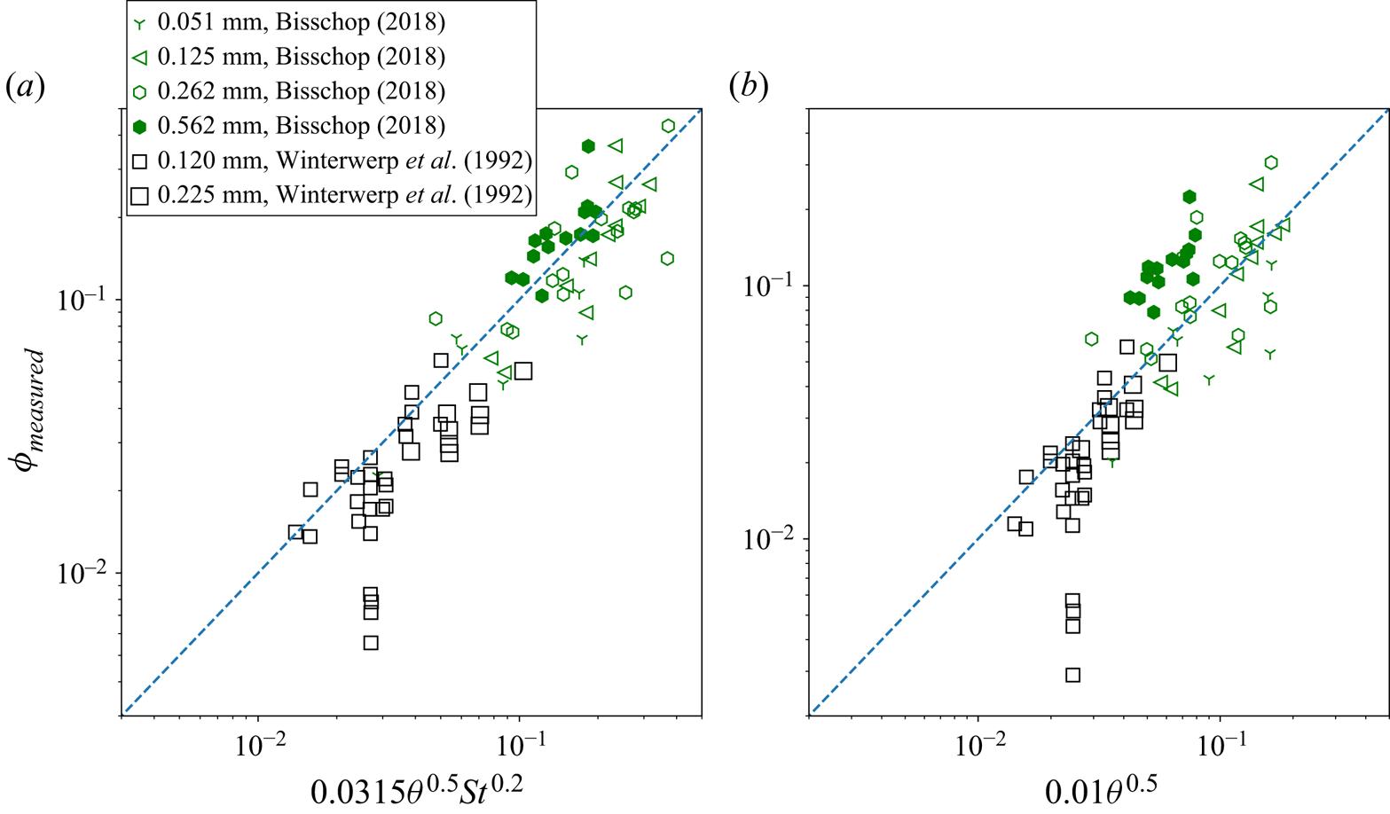
Figure 10. Scaling of the pick-up flux at a high Shields number  $\theta >8.7$ of Bisschop (Reference Bisschop2018) and data points obtained from Winterwerp et al. (Reference Winterwerp, Bakker, Mastbergen and van Rossum1992). Pick-up flux (a) evaluated at a fixed reference height $y_r=3$ cm above the bed ( $y_r/h=0.15$) as in Bisschop (Reference Bisschop2018), and (b) evaluated at a fixed non-dimensional reference height $St=1$ or $y_r=t_pu_*/\kappa$ and $\left \langle \alpha \right \rangle _r=0.41$. The dashed line indicates perfect correlation.
This does not mean that other explanations are not possible, such as the dilatancy hardening effect; see § 1. The pore pressure just below the bed and prior to pick-up is difficult to measure and therefore not available. However, using the estimate for the critical Shields parameter  $\theta _{cr}$ corrected for the dilatancy effect by the theory of Van Rhee (Reference Van Rhee2010), it is verified that $\theta _{cr}\ll \theta$. This suggest that dilatancy hardening could be present, but it is unlikely that it affected the pick-up rate in the experiments considered here. Another explanation proposed by van Rijn et al. (Reference van Rijn, Bisschop and van Rhee2019), as discussed briefly in § 1, is that the pick-up flux at high Shields numbers is reduced by a higher effective viscosity of the mixture of water and particles. In the context of this study, we need to substitute the effective mixture viscosity in (2.14). In summary, changes in the relative importance of terms in the TKE budget under high Shields conditions are a plausible explanation for the scaling anomaly observed in figure 2.
5. Conclusion
In this paper, the physical origin of several empirical scaling laws for the sediment pick-up flux has been investigated by considering the turbulent kinetic energy (TKE) balances for a stratified single-phase flow under the Boussinesq approximation and a full two-phase flow formulation. The scaling relations derived from the aforementioned balances are tested against existing erosion experiments.
At low Shields number,  $\theta <0.15$, the probability of pick-up of a single particle by the overlying turbulent flow strongly depends on the Shields number. Buoyancy destruction of TKE is presumably not the dominant process in this regime.
In the range  $0.15 < \theta \lesssim 1.5$, stratification effects likely dominate the sediment pick-up process. The non-dimensional pick-up flux $\phi$ can be scaled with the particle Reynolds number based on the shear velocity and the Shields number: $\phi \propto Re_p\,\theta ^{1.5}$.
For high Shields number flow,  $\theta \gg 1$, a high near-bed concentration develops. Based on the observation of the Obukhov length in this regime, the buoyancy destruction of TKE is not the dominant process. It is anticipated that dissipation of TKE by collisions and TKE dissipation by drag become the dominant sinks and balance the shear production of TKE. From this hypothesis, a non-dimensional scaling relation is retrieved for the non-dimensional pick-up flux, $\phi \propto St^{\xi }\,\theta ^{0.5}$. From the observed sediment concentrations in the high Shields regime, a value $\xi =0.2$ is found. It is observed that the non-dimensional pick-up rate scales in accordance with this value, $\phi \propto St^{0.2}\,\theta ^{0.5}$. This scaling is confirmed by two independent data sets.
In order to further advance our understanding of erosion processes, new high-resolution measurements of near-bed sediment transport phenomena as well as interface-resolving DNS simulations of this problem are needed. These data could be used to formulate closures for both the instantaneous and Reynolds-averaged two-phase equations. The long-term goal would be to develop an accurate pick-up flux formula for large-scale morphodynamical models for riverine, coastal and offshore applications.
Declaration of interests
The authors report no conflict of interest.
Appendix A. Derivation of the TKE balances
To study the effects of high concentrations and particle slip on the TKE budget, we present in this appendix the TKE balances of single-phase flow under both the Boussinesq approximation and a full two-phase flow formulation.
In the Boussinesq approximation, it is assumed that the density differences can be ignored in the inertia terms and affect only the buoyancy of the fluid. The flow can be described by a single velocity field  $\boldsymbol {u}$ that is governed by the momentum balance
 \begin{equation} \frac{\partial\boldsymbol{u}}{\partial t}+\boldsymbol{\nabla}\boldsymbol{\cdot}(\boldsymbol{u}\boldsymbol{u}+\boldsymbol{\mathsf{P}}) =\boldsymbol{g}+\frac{\rho-\rho_0}{\rho_0}\,\boldsymbol{g}, \end{equation}
where  $\rho$ is a variable density field, and $\rho _0$ is a fixed reference density. The stress tensor $\boldsymbol{\mathsf{P}}$ is the combination of the pressure and viscous stresses:
 \begin{equation} \boldsymbol{\mathsf{P}}=\frac{1}{\rho_0}\left(p\boldsymbol{I}-\boldsymbol{\sigma}\right). \end{equation}
As the density variations are negligible under the Boussinesq approximation, it is assumed that the velocity field is incompressible:
 \begin{equation} \boldsymbol{\nabla}\boldsymbol{\cdot} \boldsymbol{u}=0. \end{equation}
Applying Reynolds decomposition,  $\boldsymbol {u}=\left \langle \boldsymbol {u} \right \rangle +\boldsymbol {u}'$, and the standard averaging rules then give an equation for the averaged velocity:
 \begin{equation} \frac{\partial\left\langle \boldsymbol{u} \right\rangle}{\partial t}+\boldsymbol{\nabla}\boldsymbol{\cdot} \left(\left\langle \boldsymbol{u} \right\rangle\left\langle \boldsymbol{u} \right\rangle+\left\langle \boldsymbol{u}'\boldsymbol{u}' \right\rangle- \frac{1}{\rho_0}\left\langle \boldsymbol{\sigma} \right\rangle\right)={-}\frac{1}{\rho_0}\, \boldsymbol{\nabla}\langle{p}\rangle+\boldsymbol{g}+\frac{\left\langle \rho \right\rangle-\rho_0}{\rho_0}\,\boldsymbol{g}. \end{equation}
Again applying Reynolds decomposition to (A1), multiplying this equation with  $\boldsymbol {u}'$ and then taking the average, gives
 \begin{align} &\frac{\partial k}{\partial t}+\boldsymbol{\nabla}\boldsymbol{\cdot} \left[\left\langle \boldsymbol{u} \right\rangle k +\left\langle \frac{1}{2}\boldsymbol{u}'(\boldsymbol{u}'\boldsymbol{\cdot} \boldsymbol{u}') \right\rangle +\frac{1}{\rho_0}\left\langle p'\boldsymbol{u}' \right\rangle-\frac{1}{\rho_0}\left\langle \boldsymbol{\sigma}'\boldsymbol{\cdot} \boldsymbol{u}' \right\rangle\right]\nonumber\\ &\quad ={-}\left\langle \boldsymbol{u}'\boldsymbol{u}' \right\rangle:\boldsymbol{\nabla}{\left\langle \boldsymbol{u} \right\rangle}- \frac{1}{\rho_0}\left\langle \boldsymbol{\nabla}\boldsymbol{u}':\boldsymbol{\sigma}' \right\rangle+ \frac{\left\langle \rho'\boldsymbol{u}' \right\rangle}{\rho_0}\boldsymbol{\cdot}\boldsymbol{g}, \end{align}
where  $k=\frac {1}{2}\left \langle \boldsymbol {u}'\boldsymbol {\cdot }\boldsymbol {u}' \right \rangle$. The terms on the left-hand side of (A5) represent the local time change, transport of TKE by the mean flow, and transport by fluctuations of velocity, pressure and viscous stress, respectively. The three terms on the right-hand side embody the shear production, viscous dissipation and buoyancy modulation, respectively.
For higher concentrations and to account for non-negligible velocity differences between the particle and fluid phases, we require a full two-phase formulation. In this work, we use the equations and analysis of Fox (Reference Fox2014) as a starting point. The instantaneous mass and momentum equations of the particle and fluid phase read
 \begin{equation} \frac{\partial\alpha}{\partial t}+\boldsymbol{\nabla}\boldsymbol{\cdot} \left(\alpha \boldsymbol{u}_p\right)=0 \end{equation}
and
 \begin{equation} \frac{\partial\alpha\boldsymbol{u}_p}{\partial t}+\boldsymbol{\nabla}\boldsymbol{\cdot}\alpha \left(\boldsymbol{u}_p\boldsymbol{u}_p+\boldsymbol{\mathsf{P}}_{\boldsymbol{p}}\right)=\alpha\left(\mathcal{A}+\boldsymbol{g}\right), \end{equation}
respectively, where  $\alpha$ is the phase fraction, $\boldsymbol {u}_p$ is the velocity of the particle phase, $\boldsymbol{\mathsf{P}}_{\boldsymbol{p}}$ is the collisional stress tensor, $\boldsymbol {g}$ is the gravitational acceleration, and
 \begin{equation} \mathcal{A}=\frac{1}{t_p}\left(\boldsymbol{u}_f-\boldsymbol{u}_p\right)-\frac{1}{\rho_p}\,\boldsymbol{\nabla} p_f \end{equation}
represents the momentum exchange between the phases via drag and pressure, where  $t_p$ is a drag time scale. The fluid phase equations have a similar form for mass,
 \begin{equation} \frac{\partial(1-\alpha)}{\partial t}+\boldsymbol{\nabla}\boldsymbol{\cdot}\left( (1-\alpha)\boldsymbol{u}_f\right)=0 , \end{equation}
and momentum,
 \begin{equation} \frac{\partial(1-\alpha)\boldsymbol{u}_f}{\partial t}+\boldsymbol{\nabla} \boldsymbol{\cdot} (1-\alpha)\left(\boldsymbol{u}_f\boldsymbol{u}_f+\boldsymbol{\mathsf{P}}_f \right)={-}\frac{\rho_p}{\rho_f}\,\alpha \mathcal{A}+(1-\alpha)\boldsymbol{g}, \end{equation}
where  $\boldsymbol {u}_f$ is the velocity of the fluid phase, and $\boldsymbol{\mathsf{P}}_f$ is the combination of the fluid pressure and fluid viscous stress:
 \begin{equation} \boldsymbol{\mathsf{P}}_f=\frac{1}{\rho_f(1-\alpha)}\left(p_f\boldsymbol{\mathsf{I}}-\boldsymbol{\sigma}_f\right). \end{equation}
Reynolds averaging of the particle and fluid mass balances, (A6) and (A9), gives
 \begin{equation} \frac{\partial\langle{\alpha}\rangle}{\partial t}+\boldsymbol{\nabla}\boldsymbol{\cdot}\left\langle \alpha \right\rangle\left\langle \boldsymbol{u}_p \right\rangle_p=0 \end{equation}
and
 \begin{equation} \frac{\partial\langle{1-\alpha}\rangle}{\partial t}+\boldsymbol{\nabla}\boldsymbol{\cdot}\left\langle 1-\alpha \right\rangle\left\langle \boldsymbol{u}_f \right\rangle_f=0, \end{equation}
where  $\left \langle A \right \rangle$ denotes standard Reynolds averaging of a quantity $A$,
$A$,  $\left \langle A \right \rangle _p=\left \langle \alpha A \right \rangle /\left \langle \alpha \right \rangle$ is a particle-phase-weighted average, and $\left \langle A \right \rangle _f=\left \langle (1-\alpha ) A \right \rangle /\left \langle 1-\alpha \right \rangle$ is a fluid-phase- weighted average. These averages $\left \langle \cdot \right \rangle _f$ and $\left \langle \cdot \right \rangle _p$ can be interpreted as averages as ‘seen’ by the fluid and the particle phase, respectively.
Averaging (A7) gives the Reynolds-averaged momentum balance of the particles:
 \begin{align} &\frac{\partial\langle{\alpha}\rangle\left\langle \boldsymbol{u}_p \right\rangle_p}{\partial t}+\boldsymbol{\nabla}\boldsymbol{\cdot} \left\langle \alpha \right\rangle\left(\left\langle \boldsymbol{u}_p \right\rangle_p\left\langle \boldsymbol{u}_p \right\rangle_p+\left\langle \boldsymbol{u}_p''\boldsymbol{u}_p'' \right\rangle_p+\left\langle \boldsymbol{\mathsf{P}}_p \right\rangle_p\right) \nonumber\\ &\quad =\frac{\left\langle \alpha \right\rangle}{t_p}\left(\left\langle \boldsymbol{u}_f \right\rangle_f-\left\langle \boldsymbol{u}_p \right\rangle_p+\frac{\left\langle \alpha' \boldsymbol{u}_f' \right\rangle}{\left\langle \alpha \right\rangle\left\langle 1-\alpha \right\rangle} \right)-\frac{\left\langle \alpha \right\rangle}{\rho_p}\,\boldsymbol{\nabla} \left\langle p_f \right\rangle-\frac{1}{\rho_p}\left\langle \alpha'\boldsymbol{\nabla} p_f' \right\rangle+\left\langle \alpha \right\rangle\boldsymbol{g}, \end{align}
where  $A'=A-\left \langle A \right \rangle$ is the fluctuation with respect to the usual Reynolds-averaged value, and $A''=A-\left \langle A \right \rangle _p$ is the fluctuation with respect to the particle-phase-weighted average. Fluctuations in the time scale $t_p$ are ignored for the sake of simplicity.
Averaging (A10) gives the averaged momentum balance for the fluid phase:
 \begin{align} &\frac{\partial\langle 1-\alpha \rangle \left\langle \boldsymbol{u}_f\right\rangle_f}{\partial t}+ \boldsymbol{\nabla}\boldsymbol{\cdot} \left( \left\langle 1-\alpha \right\rangle\left\langle \boldsymbol{u}_f\right\rangle_f\left\langle \boldsymbol{u}_f\right\rangle_f+\left\langle 1-\alpha\right\rangle \left\langle\boldsymbol{u}_f^{\prime\prime\prime}\boldsymbol{u}_f^{\prime\prime\prime} \right\rangle _f -\frac{1}{\rho_f}\left\langle \boldsymbol{\sigma}_f \right\rangle\right)\nonumber\\ &\quad =\frac{\rho_p \left\langle\alpha\right\rangle}{\rho_f t_p}\left(\left\langle\boldsymbol{u_p}\right\rangle_p-\left\langle \boldsymbol{u_f}\right\rangle_f-\frac{\left\langle\alpha'\boldsymbol{u}_f{'}\right\rangle}{ \left\langle\alpha\right\rangle\left\langle 1-\alpha\right\rangle} \right) -\frac{\left\langle 1-\alpha \right\rangle}{\rho_f}\,{\boldsymbol{\nabla} \left\langle p_f \right\rangle}+\frac{1}{\rho_f}\left\langle \alpha'\,\boldsymbol{\nabla} p_f' \right\rangle+\left\langle 1-\alpha \right\rangle\boldsymbol{g}, \end{align}
where  $A'''=A-\left \langle A \right \rangle _f$ represents fluctuations of a quantity $A$ with respect to the fluid-phase-weighted average. Several useful relations are available to convert easily between the different types of averages; see table 2.
Table 2. Conversion relations between averages.
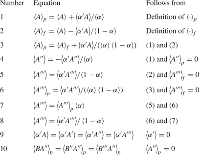
The TKE of the fluid phase and TKE of the particle phase are now defined as
 \begin{equation} k_f=\tfrac{1}{2}\left\langle \boldsymbol{u}_f'''\boldsymbol{\cdot}\boldsymbol{u}_f''' \right\rangle_f \end{equation}
and
 \begin{equation} k_p=\tfrac{1}{2}\left\langle \boldsymbol{u}_p''\boldsymbol{\cdot}\boldsymbol{u}_p'' \right\rangle_p, \end{equation}
respectively. These definitions can be interpreted as separated metrics for the TKE as seen by the fluid and particle phases individually.
The procedure to derive equations for  $k_f$ and $k_p$ from the instantaneous momentum equations is similar to the single-phase $k$ balance under the Boussinesq approximation (A5): decompose the fluid velocity field $\boldsymbol {u}_f=\left \langle \boldsymbol {u}_f \right \rangle _f+\boldsymbol {u}_f'''$ in (A10), multiply this equation with $\boldsymbol {u}_f'''$, and take the fluid average $\left \langle \cdot \right \rangle _f$:
 \begin{align} &\frac{\partial\langle{1-\alpha}\rangle\,k_f}{\partial t}+
\boldsymbol{\nabla}\boldsymbol{\cdot}\left[ \left\langle
1-\alpha \right\rangle\left\langle \boldsymbol{u}_f
\right\rangle_fk_f +\left\langle 1-\alpha
\right\rangle\frac{1}{2}\left\langle
\boldsymbol{u}_f'''\boldsymbol{u}_f'''\boldsymbol{\cdot}\boldsymbol{u}_f'''
\right\rangle_f\right.\nonumber\\ &\qquad \left.+\frac{1}{\rho_f}\left\langle
p_f\boldsymbol{u}_f''' \right\rangle
-\frac{1}{\rho_f}\left\langle
\boldsymbol{\sigma}_f\boldsymbol{\cdot}\boldsymbol{u}_f'''
\right\rangle \right]\nonumber\\ &\quad ={-}\left\langle
1-\alpha \right\rangle\left\langle
\boldsymbol{u}_f'''\boldsymbol{u}_f'''
\right\rangle_f:\boldsymbol{\nabla}\left\langle
\boldsymbol{u}_f \right\rangle_f
+\frac{1}{\rho_f}\left\langle
p_f\left(\boldsymbol{\nabla}\boldsymbol{\cdot}\boldsymbol{u}_f'''\right)
\right\rangle -\frac{1}{\rho_f}\left\langle
\boldsymbol{\nabla}
\boldsymbol{u}_f''':\boldsymbol{\sigma}_f
\right\rangle\nonumber\\ &\qquad+\frac{\rho_p\left\langle
\alpha \right\rangle}{\rho_f t_p}\left[\frac{\left\langle
\alpha'\boldsymbol{u}_f''' \right\rangle}{\left\langle
\alpha \right\rangle \left\langle 1-\alpha
\right\rangle}\left(\left\langle \boldsymbol{u}_p
\right\rangle_p-\left\langle \boldsymbol{u}_f
\right\rangle_f\right)+\left\langle
\boldsymbol{u}_f'''\boldsymbol{\cdot}\boldsymbol{u}_p''
\right\rangle_p-2k_f-\frac{\left\langle
\alpha'\boldsymbol{u}_f'''
\boldsymbol{\cdot}\boldsymbol{u}_f'''
\right\rangle}{\left\langle \alpha
\right\rangle\left\langle 1-\alpha
\right\rangle}\right]\nonumber\\ &\qquad
+\frac{1}{\rho_f\left\langle 1-\alpha
\right\rangle}\left\langle \alpha'\boldsymbol{u}_f'''
\right\rangle\boldsymbol{\cdot}\boldsymbol{\nabla}\left\langle
p_f \right\rangle+ \frac{\left\langle \alpha
\right\rangle}{\rho_f}\left(\left\langle
\boldsymbol{u}_f'''\boldsymbol{\cdot}\boldsymbol{\nabla}
p_f' \right\rangle_f+\frac{1}{\left\langle 1-\alpha
\right\rangle\left\langle \alpha \right\rangle}\left\langle
\alpha'\boldsymbol{u}_f'''\boldsymbol{\cdot}\boldsymbol{\nabla}
p_f' \right\rangle\right).
\end{align}
\begin{align} &\frac{\partial\langle{1-\alpha}\rangle\,k_f}{\partial t}+
\boldsymbol{\nabla}\boldsymbol{\cdot}\left[ \left\langle
1-\alpha \right\rangle\left\langle \boldsymbol{u}_f
\right\rangle_fk_f +\left\langle 1-\alpha
\right\rangle\frac{1}{2}\left\langle
\boldsymbol{u}_f'''\boldsymbol{u}_f'''\boldsymbol{\cdot}\boldsymbol{u}_f'''
\right\rangle_f\right.\nonumber\\ &\qquad \left.+\frac{1}{\rho_f}\left\langle
p_f\boldsymbol{u}_f''' \right\rangle
-\frac{1}{\rho_f}\left\langle
\boldsymbol{\sigma}_f\boldsymbol{\cdot}\boldsymbol{u}_f'''
\right\rangle \right]\nonumber\\ &\quad ={-}\left\langle
1-\alpha \right\rangle\left\langle
\boldsymbol{u}_f'''\boldsymbol{u}_f'''
\right\rangle_f:\boldsymbol{\nabla}\left\langle
\boldsymbol{u}_f \right\rangle_f
+\frac{1}{\rho_f}\left\langle
p_f\left(\boldsymbol{\nabla}\boldsymbol{\cdot}\boldsymbol{u}_f'''\right)
\right\rangle -\frac{1}{\rho_f}\left\langle
\boldsymbol{\nabla}
\boldsymbol{u}_f''':\boldsymbol{\sigma}_f
\right\rangle\nonumber\\ &\qquad+\frac{\rho_p\left\langle
\alpha \right\rangle}{\rho_f t_p}\left[\frac{\left\langle
\alpha'\boldsymbol{u}_f''' \right\rangle}{\left\langle
\alpha \right\rangle \left\langle 1-\alpha
\right\rangle}\left(\left\langle \boldsymbol{u}_p
\right\rangle_p-\left\langle \boldsymbol{u}_f
\right\rangle_f\right)+\left\langle
\boldsymbol{u}_f'''\boldsymbol{\cdot}\boldsymbol{u}_p''
\right\rangle_p-2k_f-\frac{\left\langle
\alpha'\boldsymbol{u}_f'''
\boldsymbol{\cdot}\boldsymbol{u}_f'''
\right\rangle}{\left\langle \alpha
\right\rangle\left\langle 1-\alpha
\right\rangle}\right]\nonumber\\ &\qquad
+\frac{1}{\rho_f\left\langle 1-\alpha
\right\rangle}\left\langle \alpha'\boldsymbol{u}_f'''
\right\rangle\boldsymbol{\cdot}\boldsymbol{\nabla}\left\langle
p_f \right\rangle+ \frac{\left\langle \alpha
\right\rangle}{\rho_f}\left(\left\langle
\boldsymbol{u}_f'''\boldsymbol{\cdot}\boldsymbol{\nabla}
p_f' \right\rangle_f+\frac{1}{\left\langle 1-\alpha
\right\rangle\left\langle \alpha \right\rangle}\left\langle
\alpha'\boldsymbol{u}_f'''\boldsymbol{\cdot}\boldsymbol{\nabla}
p_f' \right\rangle\right).
\end{align}
Likewise, the equation for  $k_p$ can be found by multiplying the instantaneous momentum equations of the particles (A7) with $\boldsymbol {u}_p''$ and taking the average $\left \langle \cdot \right \rangle _p$:
 \begin{align} &\frac{\partial\langle{\alpha}\rangle\,k_p}{\partial t}+\boldsymbol{\nabla}\boldsymbol{\cdot}\left\langle \alpha \right\rangle\left(k_p\left\langle \boldsymbol{u}_p \right\rangle_p + \frac{1}{2}\left\langle \boldsymbol{u}_p''\boldsymbol{u}_p''\boldsymbol{\cdot}\boldsymbol{u}_p'' \right\rangle_p+\left\langle \boldsymbol{\mathsf{P}}_p\boldsymbol{\cdot}\boldsymbol{u}_p'' \right\rangle_p\right) \nonumber\\ &\quad ={-}\left\langle \alpha \right\rangle\left\langle \boldsymbol{u}_p''\boldsymbol{u}_p'' \right\rangle_p:\boldsymbol{\nabla}\left\langle \boldsymbol{u}_p \right\rangle_p+\left\langle \alpha \right\rangle\left\langle \boldsymbol{\mathsf{P}}_p:\boldsymbol{\nabla} \boldsymbol{u}_p'' \right\rangle_p\nonumber\\ &\qquad + \frac{\left\langle \alpha \right\rangle}{t_p}\left(\left\langle \boldsymbol{u}_p''\boldsymbol{\cdot} \boldsymbol{u}_f'' \right\rangle_p-2k_p \right)-\frac{\left\langle \alpha \right\rangle}{\rho_p}\left\langle \boldsymbol{u}_p''\boldsymbol{\cdot}\boldsymbol{\nabla}p_f' \right\rangle_p. \end{align}
Fox (Reference Fox2014) reports the  $k_f$ and $k_p$ equations exactly in these forms, which served as the starting point for a discussion on closure relations there. A buoyancy term as in (A5) cannot be recognized in either (A18) or (A19). Fox (Reference Fox2014) argues that the buoyancy is hidden in the averaged and fluctuating pressure gradient terms, thereby assuming a quasi-hydrostatic balance
 \begin{equation} \boldsymbol{\nabla} p_f=\boldsymbol{\nabla}{\left\langle p_f \right\rangle}+ \boldsymbol{\nabla}{{p_f'}}\approx\rho_m\boldsymbol{g}+\alpha'(\rho_p-\rho_f)\boldsymbol{g}. \end{equation}
However, even with this strong assumption, it is not transparent how the Boussinesq form (A5) should appear as a limiting case of (A18) and (A19). Therefore, we try to rewrite (A18) and (A19) to allow for a more direct comparison with (A5) in the following steps.
First, focus on the transport term  $\boldsymbol {\nabla }\boldsymbol {\cdot } {1}/{\rho _f}\left \langle p_f\boldsymbol {u}_f''' \right \rangle$ on the left-hand side of (A18). Using Reynolds decomposition of the fluid pressure gives
 \begin{align} \boldsymbol{\nabla}\boldsymbol{\cdot}\frac{1}{\rho_f}\left\langle p_f\boldsymbol{u}_f''' \right\rangle &=\boldsymbol{\nabla}\boldsymbol{\cdot}\frac{1}{\rho_f}\left\langle \left(\left\langle p_f \right\rangle+p_f'\right)\boldsymbol{u}_f''' \right\rangle= \boldsymbol{\nabla}\boldsymbol{\cdot}\frac{1}{\rho_f}\left\langle p_f \right\rangle\left\langle \boldsymbol{u}_f''' \right\rangle+ \boldsymbol{\nabla}\boldsymbol{\cdot}\frac{1}{\rho_f}\left\langle p_f'\boldsymbol{u}_f''' \right\rangle\nonumber\\ & =\frac{1}{\rho_f}\left\langle p_f \right\rangle\boldsymbol{\nabla}\boldsymbol{\cdot}{\left\langle \boldsymbol{u}_f''' \right\rangle}+ \frac{1}{\rho_f}\left\langle \boldsymbol{u}_f''' \right\rangle\boldsymbol{\cdot}\boldsymbol{\nabla}\left\langle p_f \right\rangle+ \boldsymbol{\nabla}\boldsymbol{\cdot}\frac{1}{\rho_f}\left\langle p_f'\boldsymbol{u}_f''' \right\rangle\nonumber\\ &=\frac{1}{\rho_f}\left\langle p_f \right\rangle\boldsymbol{\nabla}\boldsymbol{\cdot}{\left\langle \boldsymbol{u}_f''' \right\rangle}+ \frac{1}{\rho_f\left\langle 1-\alpha \right\rangle}\left\langle \alpha'\boldsymbol{u}_f''' \right\rangle\boldsymbol{\cdot}\boldsymbol{\nabla} \left\langle p_f \right\rangle+\boldsymbol{\nabla}\boldsymbol{\cdot}\frac{1}{\rho_f}\left\langle p_f'\boldsymbol{u}_f''' \right\rangle, \end{align}
where we used relation 8 from table 2 to convert  $\left \langle \boldsymbol {u}_f''' \right \rangle$.
The second term on the right-hand side of (A18) can also be rewritten using Reynolds decomposition of  $p_f$:
 \begin{align} \frac{1}{\rho_f}\left\langle p_f\,\left(\boldsymbol{\nabla}\boldsymbol{\cdot}\boldsymbol{u}_f''' \right) \right\rangle& =\frac{1}{\rho_f}\left\langle \left(\left\langle p_f \right\rangle+p_f'\right)\left(\boldsymbol{\nabla}\boldsymbol{\cdot}\boldsymbol{u}_f''' \right) \right\rangle\nonumber\\ &=\frac{1}{\rho_f}\left\langle p_f \right\rangle\boldsymbol{\nabla}\boldsymbol{\cdot}\left\langle \boldsymbol{u}_f''' \right\rangle+ \frac{1}{\rho_f}\left\langle p_f'\,\left(\boldsymbol{\nabla}\boldsymbol{\cdot}\boldsymbol{u}_f'''\right) \right\rangle. \end{align}
The last term on the right-hand side of (A18) can be reorganized using relation 3 of table 2 and the chain rule:
 \begin{align} \frac{\left\langle \alpha \right\rangle}{\rho_f}\left(\left\langle \boldsymbol{u}_f'''\boldsymbol{\cdot}\boldsymbol{\nabla} p_f' \right\rangle_f+\frac{1}{ \left\langle 1-\alpha \right\rangle\left\langle \alpha \right\rangle}\left\langle \alpha'\boldsymbol{u}_f'''\boldsymbol{\cdot}\boldsymbol{\nabla} p_f' \right\rangle\right) &=\frac{\left\langle \alpha \right\rangle}{\rho_f}\left\langle \boldsymbol{u}_f'''\boldsymbol{\cdot}\boldsymbol{\nabla} p_f' \right\rangle_p\nonumber\\ &=\frac{1}{\rho_f}\left\langle \alpha\boldsymbol{u}_f'''\boldsymbol{\cdot}\boldsymbol{\nabla} p_f' \right\rangle\nonumber\\ &=\frac{1}{\rho_f} \boldsymbol{\nabla}\boldsymbol{\cdot} \left\langle \alpha\boldsymbol{u}_f'''p_f' \right\rangle-\frac{1}{ \rho_f} \left\langle p_f'\,\boldsymbol{\nabla}\boldsymbol{\cdot}\alpha \boldsymbol{u}_f''' \right\rangle, \end{align}
which demonstrates that it constitutes a transport term and a compression term. Likewise, the last term on the right-hand side of the particle TKE balance (A19) can also be expressed as the sum of a transport term and a compression term:
 \begin{align} \frac{\left\langle \alpha \right\rangle}{\rho_p}\left\langle \boldsymbol{u}_p''\boldsymbol{\cdot}\boldsymbol{\nabla} p_f' \right\rangle_p&=\frac{1}{\rho_p}\boldsymbol{\nabla}\boldsymbol{\cdot} \left\langle \alpha \right\rangle\left\langle p_f'\boldsymbol{u}_p'' \right\rangle_p-\frac{1}{\rho_p}\left\langle p_f'\left(\boldsymbol{\nabla}\boldsymbol{\cdot}\alpha \boldsymbol{u}_p''\right) \right\rangle\nonumber\\ &=\frac{1}{\rho_p}\,\boldsymbol{\nabla}\boldsymbol{\cdot}\left\langle \alpha \boldsymbol{u}_p''p_f' \right\rangle-\frac{1}{\rho_p}\left\langle p_f'\left(\boldsymbol{\nabla}\boldsymbol{\cdot}\alpha \boldsymbol{u}_p''\right) \right\rangle. \end{align}
The contribution of the drag force in (A18) can also be written as
 \begin{align} &\frac{\rho_p\left\langle \alpha \right\rangle}{\rho_f t_p}\left[\frac{\left\langle \alpha'\boldsymbol{u}_f''' \right\rangle}{\left\langle \alpha \right\rangle\left\langle 1-\alpha \right\rangle}\left(\left\langle \boldsymbol{u}_p \right\rangle_p- \left\langle \boldsymbol{u}_f \right\rangle_f\right)+\left\langle \boldsymbol{u}_f'''\boldsymbol{\cdot} \boldsymbol{u}_p'' \right\rangle_p-2k_f-\frac{\left\langle \alpha'\boldsymbol{u}_f'''\boldsymbol{\cdot}\boldsymbol{u}_f''' \right\rangle}{\left\langle \alpha \right\rangle\left\langle 1-\alpha \right\rangle}\right]\nonumber\\ &\quad =\frac{\rho_p\left\langle \alpha \right\rangle}{\rho_f t_p}\left[\frac{\left\langle \alpha'\boldsymbol{u}_f''' \right\rangle}{\left\langle \alpha \right\rangle\left\langle 1-\alpha \right\rangle}\left(\left\langle \boldsymbol{u}_p \right\rangle_p- \left\langle \boldsymbol{u}_f \right\rangle_f\right)+\left\langle \boldsymbol{u}_f'''\boldsymbol{\cdot} \boldsymbol{u}_p'' \right\rangle_p-\left\langle \boldsymbol{u}_f'''\boldsymbol{\cdot}\boldsymbol{u}_f''' \right\rangle_p\right]\nonumber\\ &\quad =\frac{\rho_p\left\langle \alpha \right\rangle}{\rho_f t_p}\left[\frac{\left\langle \alpha'\boldsymbol{u}_f' \right\rangle}{\left\langle \alpha \right\rangle\left\langle 1-\alpha \right\rangle} \boldsymbol{\cdot}\left(\left\langle \boldsymbol{u}_p \right\rangle_p-\left\langle \boldsymbol{u}_f \right\rangle_f- \frac{\left\langle \alpha'\boldsymbol{u}_f' \right\rangle}{\left\langle \alpha \right\rangle\left\langle 1-\alpha \right\rangle}\right)+ \left\langle \boldsymbol{u}_f''\boldsymbol{\cdot}\boldsymbol{u}_p'' \right\rangle_p-\left\langle \boldsymbol{u}_f''\boldsymbol{\cdot} \boldsymbol{u}_f'' \right\rangle_p\right], \end{align}
where we used in the first step conversion 3 in table 2 for the definition of  $k_f$,
 \begin{equation} \left\langle \boldsymbol{u}_f'''\boldsymbol{\cdot}\boldsymbol{u}_f''' \right\rangle_p=\left\langle \boldsymbol{u}_f'''\boldsymbol{\cdot}\boldsymbol{u}_f''' \right\rangle_f+ \frac{\left\langle \alpha'\boldsymbol{u}_f'''\boldsymbol{\cdot}\boldsymbol{u}_f''' \right\rangle}{\left\langle \alpha \right\rangle\left\langle 1-\alpha \right\rangle}= 2k_f+\frac{\left\langle \alpha'\boldsymbol{u}_f'''\boldsymbol{\cdot}\boldsymbol{u}_f''' \right\rangle}{\left\langle \alpha \right\rangle\left\langle 1-\alpha \right\rangle}, \end{equation}
and in the second step,
 \begin{align} \left\langle \boldsymbol{u}_f'''\boldsymbol{\cdot}\boldsymbol{u}_f''' \right\rangle_p&=\frac{\left\langle \alpha\left(\boldsymbol{u}_f-\left\langle \boldsymbol{u}_f \right\rangle_f\right) \boldsymbol{\cdot}\left(\boldsymbol{u}_f-\left\langle \boldsymbol{u}_f \right\rangle_f\right) \right\rangle}{\left\langle \alpha \right\rangle}\nonumber\\ &=\frac{\left\langle \alpha\left(\left\langle \boldsymbol{u}_f \right\rangle_p+\boldsymbol{u}_f''-\left\langle \boldsymbol{u}_f \right\rangle_f\right) \boldsymbol{\cdot}\left(\left\langle \boldsymbol{u}_f \right\rangle_p+\boldsymbol{u}_f''-\left\langle \boldsymbol{u}_f \right\rangle_f\right) \right\rangle}{\left\langle \alpha \right\rangle}\nonumber\\ &=\frac{\left\langle \alpha\left[\left\langle \boldsymbol{u}_f \right\rangle_p-\left\langle \boldsymbol{u}_f \right\rangle_f+\boldsymbol{u}_f''\right] \boldsymbol{\cdot}\left[\left\langle \boldsymbol{u}_f \right\rangle_p-\left\langle \boldsymbol{u}_f \right\rangle_f+\boldsymbol{u}_f''\right] \right\rangle}{\left\langle \alpha \right\rangle}\nonumber\\ &=\frac{\left\langle \alpha\left[\left\langle \boldsymbol{u}_f \right\rangle_p-\left\langle \boldsymbol{u}_f \right\rangle_f\right]\boldsymbol{\cdot} \left[\left\langle \boldsymbol{u}_f \right\rangle_p-\left\langle \boldsymbol{u}_f \right\rangle_f\right] \right\rangle}{\left\langle \alpha \right\rangle}\nonumber\\ &\quad +\frac{\left\langle \alpha \boldsymbol{u}_f''\boldsymbol{\cdot}\boldsymbol{u}_f'' \right\rangle}{\left\langle \alpha \right\rangle}+ 2\,\frac{\left\langle \alpha\boldsymbol{u}_f''\boldsymbol{\cdot}\left[\left\langle \boldsymbol{u}_f \right\rangle_p-\left\langle \boldsymbol{u}_f \right\rangle_f\right] \right\rangle}{\left\langle \alpha \right\rangle}\nonumber\\ &=\left|\left\langle \boldsymbol{u}_f \right\rangle_p-\left\langle \boldsymbol{u}_f \right\rangle_f\right|^2+\left\langle \boldsymbol{u}_f''\boldsymbol{\cdot} \boldsymbol{u}_f'' \right\rangle_p+2\,\frac{\left\langle \alpha\boldsymbol{u}_f'' \right\rangle\boldsymbol{\cdot}\left[\left\langle \boldsymbol{u}_f \right\rangle_p-\left\langle \boldsymbol{u}_f \right\rangle_f\right]}{\left\langle \alpha \right\rangle}\nonumber\\ &=\left|\left\langle \boldsymbol{u}_f \right\rangle_p-\left\langle \boldsymbol{u}_f \right\rangle_f\right|^2+\left\langle \boldsymbol{u}_f''\boldsymbol{\cdot}\boldsymbol{u}_f'' \right\rangle_p+0\nonumber\\ &=\left|\frac{\left\langle \alpha'\boldsymbol{u}_f' \right\rangle}{\left\langle \alpha \right\rangle\left\langle 1-\alpha \right\rangle}\right|^2+\left\langle \boldsymbol{u}_f''\boldsymbol{\cdot}\boldsymbol{u}_f'' \right\rangle_p, \end{align}
and from table 2 conversion 10,
 \begin{equation} \left\langle \boldsymbol{u}_f'''\boldsymbol{\cdot}\boldsymbol{u}_p'' \right\rangle_p=\left\langle \boldsymbol{u}_f''\boldsymbol{\cdot}\boldsymbol{u}_p'' \right\rangle_p. \end{equation}
Substitution of the re-expressed terms (A21), (A22), (A23) and (A25) into the  $k_f$ balance (A18) gives
 \begin{align} &\frac{\partial\rho_f\left\langle 1-\alpha \right\rangle
k_f}{\partial t} +\boldsymbol{\nabla}\boldsymbol{\cdot} \left[
\rho_f\left\langle 1-\alpha \right\rangle\left\langle
\boldsymbol{u}_f \right\rangle_fk_f +\rho_f\left\langle
1-\alpha \right\rangle\frac{1}{2}\left\langle
\boldsymbol{u}_f'''\boldsymbol{u}_f'''\boldsymbol{\cdot}\boldsymbol{u}_f'''
\right\rangle_f\right.\nonumber\\ &\qquad \left. +{\left\langle 1-\alpha
\right\rangle}\left\langle p_f'\boldsymbol{u}_f'''
\right\rangle_f -\left\langle
\boldsymbol{\sigma}_f\boldsymbol{\cdot}\boldsymbol{u}_f'''
\right\rangle\right]\nonumber\\ &\quad ={-}\left\langle
1-\alpha \right\rangle\rho_f\left\langle
\boldsymbol{u}_f'''\boldsymbol{u}_f'''
\right\rangle_f:\boldsymbol{\nabla}\left\langle
\boldsymbol{u}_f \right\rangle_f +\left\langle
p_f'\left(\boldsymbol{\nabla}\boldsymbol{\cdot}(1-\alpha)\boldsymbol{u}_f'''\right)
\right\rangle -\left\langle
\boldsymbol{\nabla}\boldsymbol{u}_f''':\boldsymbol{\sigma}_f
\right\rangle\nonumber\\ &\qquad +\frac{\rho_p\left\langle
\alpha \right\rangle}{ t_p}\left[\!\frac{\left\langle
\alpha'\boldsymbol{u}_f' \right\rangle}{\left\langle \alpha
\right\rangle\left\langle 1-\alpha \right\rangle}
\boldsymbol{\cdot}\left(\!\left\langle \boldsymbol{u}_p
\right\rangle_p-\left\langle \boldsymbol{u}_f
\right\rangle_f-\frac{\left\langle \alpha'\boldsymbol{u}_f'
\right\rangle}{\left\langle \alpha
\right\rangle\left\langle 1-\alpha
\right\rangle}\!\right)+\left\langle \boldsymbol{u}_f''
\boldsymbol{\cdot}\boldsymbol{u}_p''
\right\rangle_p-\left\langle
\boldsymbol{u}_f''\boldsymbol{\cdot} \boldsymbol{u}_f''
\right\rangle_p\!\right]\!,
\end{align}
\begin{align} &\frac{\partial\rho_f\left\langle 1-\alpha \right\rangle
k_f}{\partial t} +\boldsymbol{\nabla}\boldsymbol{\cdot} \left[
\rho_f\left\langle 1-\alpha \right\rangle\left\langle
\boldsymbol{u}_f \right\rangle_fk_f +\rho_f\left\langle
1-\alpha \right\rangle\frac{1}{2}\left\langle
\boldsymbol{u}_f'''\boldsymbol{u}_f'''\boldsymbol{\cdot}\boldsymbol{u}_f'''
\right\rangle_f\right.\nonumber\\ &\qquad \left. +{\left\langle 1-\alpha
\right\rangle}\left\langle p_f'\boldsymbol{u}_f'''
\right\rangle_f -\left\langle
\boldsymbol{\sigma}_f\boldsymbol{\cdot}\boldsymbol{u}_f'''
\right\rangle\right]\nonumber\\ &\quad ={-}\left\langle
1-\alpha \right\rangle\rho_f\left\langle
\boldsymbol{u}_f'''\boldsymbol{u}_f'''
\right\rangle_f:\boldsymbol{\nabla}\left\langle
\boldsymbol{u}_f \right\rangle_f +\left\langle
p_f'\left(\boldsymbol{\nabla}\boldsymbol{\cdot}(1-\alpha)\boldsymbol{u}_f'''\right)
\right\rangle -\left\langle
\boldsymbol{\nabla}\boldsymbol{u}_f''':\boldsymbol{\sigma}_f
\right\rangle\nonumber\\ &\qquad +\frac{\rho_p\left\langle
\alpha \right\rangle}{ t_p}\left[\!\frac{\left\langle
\alpha'\boldsymbol{u}_f' \right\rangle}{\left\langle \alpha
\right\rangle\left\langle 1-\alpha \right\rangle}
\boldsymbol{\cdot}\left(\!\left\langle \boldsymbol{u}_p
\right\rangle_p-\left\langle \boldsymbol{u}_f
\right\rangle_f-\frac{\left\langle \alpha'\boldsymbol{u}_f'
\right\rangle}{\left\langle \alpha
\right\rangle\left\langle 1-\alpha
\right\rangle}\!\right)+\left\langle \boldsymbol{u}_f''
\boldsymbol{\cdot}\boldsymbol{u}_p''
\right\rangle_p-\left\langle
\boldsymbol{u}_f''\boldsymbol{\cdot} \boldsymbol{u}_f''
\right\rangle_p\!\right]\!,
\end{align}and substitution of (A24) into (A19) yields
 \begin{align} &\frac{\partial\rho_p\left\langle \alpha \right\rangle k_p}{\partial t}+\boldsymbol{\nabla}\boldsymbol{\cdot}\rho_p \left\langle \alpha \right\rangle\left(k_p\left\langle \boldsymbol{u}_p \right\rangle_p +\frac{1}{2}\left\langle \boldsymbol{u}_p''\boldsymbol{u}_p''\boldsymbol{\cdot} \boldsymbol{u}_p'' \right\rangle_p+\frac{1}{\rho_p}\left\langle p_f'\boldsymbol{u}_p'' \right\rangle_p+\left\langle \boldsymbol{\mathsf{P}}_p\boldsymbol{\cdot} \boldsymbol{u}_p'' \right\rangle_p\right)\nonumber\\ &\quad ={-}\rho_p\left\langle \alpha \right\rangle\left\langle \boldsymbol{u}_p''\boldsymbol{u}_p'' \right\rangle_p:\boldsymbol{\nabla}\left\langle \boldsymbol{u}_p \right\rangle_p+\left\langle p_f'\left(\boldsymbol{\nabla} \boldsymbol{\cdot}\alpha\boldsymbol{u}_p''\right) \right\rangle+ \rho_p \left\langle \alpha \right\rangle\left\langle \boldsymbol{\mathsf{P}}_p:\boldsymbol{\nabla}\boldsymbol{u}_p'' \right\rangle_p\nonumber\\ &\qquad+ \frac{\rho_p\left\langle \alpha \right\rangle}{t_p}\left(\left\langle \boldsymbol{u}_p''\boldsymbol{\cdot}\boldsymbol{u}_f'' \right\rangle_p-2k_p \right). \end{align}
To further advance the understanding, it is helpful to compute the total TKE of the fluid–particle system,  $\rho _f\left \langle 1-\alpha \right \rangle k _f+\rho _p\left \langle \alpha \right \rangle k _p$, by summing (A29) and (A30). This summation is straightforward for most terms except for the compressibility terms on the right-hand sides of the equations:
 \begin{align} \left\langle p_f'\left(\boldsymbol{\nabla}\boldsymbol{\cdot}(1-\alpha)\boldsymbol{u}_f'''\right) \right\rangle+\left\langle p_f'\left( \boldsymbol{\nabla}\boldsymbol{\cdot}\alpha \boldsymbol{u}_p''\right) \right\rangle&=\left\langle p_f'\,\boldsymbol{\nabla}\boldsymbol{\cdot}\left((1-\alpha)\boldsymbol{u}_f'''+\alpha\boldsymbol{u}_p'' \right) \right\rangle\nonumber\\ &=\left\langle p_f'\,\boldsymbol{\nabla}\boldsymbol{\cdot}\alpha'\left(\left\langle \boldsymbol{u}_f \right\rangle_f-\left\langle \boldsymbol{u}_p \right\rangle_p\right) \right\rangle, \end{align}
where we used from the mass balances (A6) and (A9) that
 \begin{align} 0&=\boldsymbol{\nabla}\boldsymbol{\cdot}\left(\alpha\boldsymbol{u}_p+(1-\alpha)\boldsymbol{u}_f \right)\nonumber\\ &=\boldsymbol{\nabla}\boldsymbol{\cdot}\left(\alpha\left(\left\langle \boldsymbol{u}_p \right\rangle_p+\boldsymbol{u}_p''\right)+(1-\alpha) \left(\left\langle \boldsymbol{u}_f \right\rangle_f+\boldsymbol{u}_f'''\right)\right)\nonumber\\ &=\boldsymbol{\nabla}\boldsymbol{\cdot}\alpha'\left(\left\langle \boldsymbol{u}_p \right\rangle_p-\left\langle \boldsymbol{u}_f \right\rangle_f\right)+ \boldsymbol{\nabla}\boldsymbol{\cdot}\left(\alpha\boldsymbol{u}_p''+(1-\alpha)\boldsymbol{u}_f''' \right). \end{align}
Summing (A29) and (A30), and using (A32), gives
 \begin{align} &\frac{\partial\rho_f\left\langle 1-\alpha \right\rangle
k_f+\rho_p\left\langle \alpha \right\rangle k_p}{\partial t}
+\boldsymbol{\nabla}\boldsymbol{\cdot}\left[
\rho_f\left\langle 1-\alpha \right\rangle\left\langle
\boldsymbol{u}_f \right\rangle_fk_f +\rho_f\left\langle
1-\alpha \right\rangle\frac{1}{2}\left\langle
\boldsymbol{u}_f'''\boldsymbol{u}_f'''\boldsymbol{\cdot}\boldsymbol{u}_f'''
\right\rangle_f\right.\nonumber\\ &\qquad \left.+{\left\langle 1-\alpha
\right\rangle}\left\langle p_f'\boldsymbol{u}_f'''
\right\rangle_f -\left\langle
\boldsymbol{\sigma}_f\boldsymbol{\cdot}\boldsymbol{u}_f'''
\right\rangle\right] \nonumber\\ &\qquad\boldsymbol{\nabla}\boldsymbol{\cdot}\left[\rho_p\left\langle
\alpha \right\rangle \left\langle \boldsymbol{u}_p
\right\rangle_pk_p +\rho_p\left\langle \alpha
\right\rangle\frac{1}{2}\left\langle
\boldsymbol{u}_p''\boldsymbol{u}_p''
\boldsymbol{\cdot}\boldsymbol{u}_p''
\right\rangle_p+\left\langle \alpha
\right\rangle\left\langle p_f'\boldsymbol{u}_p''
\right\rangle_p+\rho_p\left\langle \alpha \right\rangle
\left\langle
\boldsymbol{\mathsf{P}}_p\boldsymbol{\cdot}\boldsymbol{u}_p''
\right\rangle_p\right]\nonumber\\ &\quad={-}\rho_f\left\langle 1-\alpha
\right\rangle\left\langle
\boldsymbol{u}_f'''\boldsymbol{u}_f'''
\right\rangle_f:\boldsymbol{\nabla}\left\langle
\boldsymbol{u}_f \right\rangle_f -\rho_p\left\langle \alpha
\right\rangle\left\langle
\boldsymbol{u}_p''\boldsymbol{u}_p''
\right\rangle_p:\boldsymbol{\nabla}\left\langle
\boldsymbol{u}_p \right\rangle_p\nonumber\\ &\qquad+\left\langle
p_f'\,\boldsymbol{\nabla}\boldsymbol{\cdot}\alpha'\left(\left\langle
\boldsymbol{u}_f \right\rangle_f-\left\langle
\boldsymbol{u}_p \right\rangle_p\right) \right\rangle +
\frac{\rho_p\left\langle \alpha \right\rangle}{
t_p}\frac{\left\langle \alpha'\boldsymbol{u}_f'
\right\rangle}{\left\langle \alpha
\right\rangle\left\langle 1-\alpha \right\rangle}
\boldsymbol{\cdot}\left(\left\langle \boldsymbol{u}_p
\right\rangle_p-\left\langle \boldsymbol{u}_f
\right\rangle_f- \frac{\left\langle
\alpha'\boldsymbol{u}_f' \right\rangle}{\left\langle \alpha
\right\rangle\left\langle 1-\alpha \right\rangle}\right)
\nonumber\\ &\qquad-\left\langle \boldsymbol{\nabla}
\boldsymbol{u}_f''':\boldsymbol{\sigma}_f \right\rangle+
\rho_p\left\langle \alpha \right\rangle\left\langle
\boldsymbol{\mathsf{P}}_p:\boldsymbol{\nabla}\boldsymbol{u}_p''
\right\rangle_p -{\frac{\rho_p\left\langle \alpha
\right\rangle}{ t_p}\left\langle
\left|\boldsymbol{u}_f''-\boldsymbol{u}_p''\right|^2
\right\rangle_p}.
\end{align}
\begin{align} &\frac{\partial\rho_f\left\langle 1-\alpha \right\rangle
k_f+\rho_p\left\langle \alpha \right\rangle k_p}{\partial t}
+\boldsymbol{\nabla}\boldsymbol{\cdot}\left[
\rho_f\left\langle 1-\alpha \right\rangle\left\langle
\boldsymbol{u}_f \right\rangle_fk_f +\rho_f\left\langle
1-\alpha \right\rangle\frac{1}{2}\left\langle
\boldsymbol{u}_f'''\boldsymbol{u}_f'''\boldsymbol{\cdot}\boldsymbol{u}_f'''
\right\rangle_f\right.\nonumber\\ &\qquad \left.+{\left\langle 1-\alpha
\right\rangle}\left\langle p_f'\boldsymbol{u}_f'''
\right\rangle_f -\left\langle
\boldsymbol{\sigma}_f\boldsymbol{\cdot}\boldsymbol{u}_f'''
\right\rangle\right] \nonumber\\ &\qquad\boldsymbol{\nabla}\boldsymbol{\cdot}\left[\rho_p\left\langle
\alpha \right\rangle \left\langle \boldsymbol{u}_p
\right\rangle_pk_p +\rho_p\left\langle \alpha
\right\rangle\frac{1}{2}\left\langle
\boldsymbol{u}_p''\boldsymbol{u}_p''
\boldsymbol{\cdot}\boldsymbol{u}_p''
\right\rangle_p+\left\langle \alpha
\right\rangle\left\langle p_f'\boldsymbol{u}_p''
\right\rangle_p+\rho_p\left\langle \alpha \right\rangle
\left\langle
\boldsymbol{\mathsf{P}}_p\boldsymbol{\cdot}\boldsymbol{u}_p''
\right\rangle_p\right]\nonumber\\ &\quad={-}\rho_f\left\langle 1-\alpha
\right\rangle\left\langle
\boldsymbol{u}_f'''\boldsymbol{u}_f'''
\right\rangle_f:\boldsymbol{\nabla}\left\langle
\boldsymbol{u}_f \right\rangle_f -\rho_p\left\langle \alpha
\right\rangle\left\langle
\boldsymbol{u}_p''\boldsymbol{u}_p''
\right\rangle_p:\boldsymbol{\nabla}\left\langle
\boldsymbol{u}_p \right\rangle_p\nonumber\\ &\qquad+\left\langle
p_f'\,\boldsymbol{\nabla}\boldsymbol{\cdot}\alpha'\left(\left\langle
\boldsymbol{u}_f \right\rangle_f-\left\langle
\boldsymbol{u}_p \right\rangle_p\right) \right\rangle +
\frac{\rho_p\left\langle \alpha \right\rangle}{
t_p}\frac{\left\langle \alpha'\boldsymbol{u}_f'
\right\rangle}{\left\langle \alpha
\right\rangle\left\langle 1-\alpha \right\rangle}
\boldsymbol{\cdot}\left(\left\langle \boldsymbol{u}_p
\right\rangle_p-\left\langle \boldsymbol{u}_f
\right\rangle_f- \frac{\left\langle
\alpha'\boldsymbol{u}_f' \right\rangle}{\left\langle \alpha
\right\rangle\left\langle 1-\alpha \right\rangle}\right)
\nonumber\\ &\qquad-\left\langle \boldsymbol{\nabla}
\boldsymbol{u}_f''':\boldsymbol{\sigma}_f \right\rangle+
\rho_p\left\langle \alpha \right\rangle\left\langle
\boldsymbol{\mathsf{P}}_p:\boldsymbol{\nabla}\boldsymbol{u}_p''
\right\rangle_p -{\frac{\rho_p\left\langle \alpha
\right\rangle}{ t_p}\left\langle
\left|\boldsymbol{u}_f''-\boldsymbol{u}_p''\right|^2
\right\rangle_p}.
\end{align}Finally, to get a good interpretation of the TKE balance (A33), it is also helpful to have a complementary balance of the MKE:
 \begin{equation} \rho_p\left\langle \alpha \right\rangle K_p+\rho_f\left\langle 1-\alpha \right\rangle K_f=\tfrac{1}{2}\rho_p\left\langle \alpha \right\rangle\left\langle \boldsymbol{u}_p \right\rangle_p\boldsymbol{\cdot} \left\langle \boldsymbol{u}_p \right\rangle_p+\tfrac{1}{2}\rho_f\left\langle 1-\alpha \right\rangle\left\langle \boldsymbol{u}_f \right\rangle_p\boldsymbol{\cdot}\left\langle \boldsymbol{u}_f \right\rangle_f. \end{equation}
This balance can be obtained by multiplication of (A14) and (A15) with  $\left \langle \boldsymbol {u}_f \right \rangle _p$ and $\left \langle \boldsymbol {u}_f \right \rangle _f$, respectively. Reorganization of the resulting terms using (A12) and (A13) yields
 \begin{align} &\frac{\partial \rho_p\left\langle \alpha \right\rangle
K_p+\rho_f\left\langle 1-\alpha \right\rangle K_f}{\partial
t}+\boldsymbol{\nabla}\boldsymbol{\cdot}\left(
\rho_f\left\langle 1-\alpha \right\rangle\left\langle
\boldsymbol{u}_f \right\rangle_fK_f+\rho_p\left\langle
\alpha \right\rangle\left\langle \boldsymbol{u}_p
\right\rangle_pK_p\right)\nonumber\\ &\qquad+\boldsymbol{\nabla}\boldsymbol{\cdot}
\left(\rho_f\left\langle 1-\alpha \right\rangle\left\langle
\boldsymbol{u}_f'''\boldsymbol{u}_f''' \right\rangle_f
\boldsymbol{\cdot}\left\langle \boldsymbol{u}_f
\right\rangle_f+\rho_p\left\langle \alpha
\right\rangle\left\langle
\boldsymbol{u}_p''\boldsymbol{u}_p'' \right\rangle_p
\boldsymbol{\cdot}\left\langle \boldsymbol{u}_p
\right\rangle_p \right)\nonumber\\ &\qquad
-\boldsymbol{\nabla}\boldsymbol{\cdot}\left(\left\langle
\sigma_f \right\rangle\boldsymbol{\cdot}\left\langle
\boldsymbol{u}_f \right\rangle_f\right)+
\boldsymbol{\nabla}\boldsymbol{\cdot}
\left(\rho_p\left\langle \alpha \right\rangle\left\langle
\boldsymbol{\mathsf{P}}_p
\right\rangle_p\boldsymbol{\cdot}\left\langle
\boldsymbol{u}_p \right\rangle_p\right)\nonumber\\ &\qquad
+\boldsymbol{\nabla}\boldsymbol{\cdot} \left(\left\langle
\alpha \right\rangle\left\langle \boldsymbol{u}_p
\right\rangle_p+\left\langle 1-\alpha
\right\rangle\left\langle \boldsymbol{u}_f
\right\rangle_f\right)\left\langle p_f \right\rangle+
\boldsymbol{\nabla}\boldsymbol{\cdot}\left(\left\langle
\boldsymbol{u}_p \right\rangle_p-\left\langle
\boldsymbol{u}_f \right\rangle_f \right)\left\langle
\alpha'p_f' \right\rangle\nonumber\\ &\quad = +\rho_f\left\langle 1\!-\!\alpha
\right\rangle\left\langle
\boldsymbol{u}_f'''\boldsymbol{u}_f'''
\right\rangle_f:\boldsymbol{\nabla}\left\langle
\boldsymbol{u}_f \right\rangle_f \!+\!\rho_p\left\langle \alpha
\right\rangle\left\langle
\boldsymbol{u}_p''\boldsymbol{u}_p''
\right\rangle_p:\boldsymbol{\nabla}\left\langle
\boldsymbol{u}_p \right\rangle_p-\!\left\langle p_f'\,
\boldsymbol{\nabla}\boldsymbol{\cdot}\alpha'\left(\!\left\langle
\boldsymbol{u}_f \right\rangle_f\!-\left\langle
\boldsymbol{u}_p \right\rangle_p\!\right)
\right\rangle\nonumber\\ &\qquad - \frac{\rho_p\left\langle
\alpha \right\rangle}{ t_p}\,\frac{\left\langle
\alpha'\boldsymbol{u}_f' \right\rangle}{\left\langle \alpha
\right\rangle\left\langle 1-\alpha
\right\rangle}\boldsymbol{\cdot} \left(\left\langle
\boldsymbol{u}_p \right\rangle_p-\left\langle
\boldsymbol{u}_f \right\rangle_f- \frac{\left\langle
\alpha'\boldsymbol{u}_f' \right\rangle}{\left\langle \alpha
\right\rangle\left\langle 1-\alpha
\right\rangle}\right)-\frac{ \rho_p\left\langle \alpha
\right\rangle}{t_p}\left|\left\langle
\boldsymbol{u}_p-\boldsymbol{u}_f
\right\rangle_p\right|^2\nonumber\\ &\qquad
+\rho_p\left\langle \alpha \right\rangle\left\langle
\boldsymbol{\mathsf{P}}_p
\right\rangle_p:\boldsymbol{\nabla}\left\langle
\boldsymbol{u}_p \right\rangle_p-\left\langle \boldsymbol{\sigma}_f
\right\rangle:\boldsymbol{\nabla}\left\langle
\boldsymbol{u}_f \right\rangle_f +\left(\rho_p\left\langle
\alpha \right\rangle\left\langle \boldsymbol{u}_p
\right\rangle_p+\rho_f\left\langle 1-\alpha
\right\rangle\left\langle \boldsymbol{u}_f
\right\rangle_f\right)\boldsymbol{\cdot}\boldsymbol{g}.
\end{align}
\begin{align} &\frac{\partial \rho_p\left\langle \alpha \right\rangle
K_p+\rho_f\left\langle 1-\alpha \right\rangle K_f}{\partial
t}+\boldsymbol{\nabla}\boldsymbol{\cdot}\left(
\rho_f\left\langle 1-\alpha \right\rangle\left\langle
\boldsymbol{u}_f \right\rangle_fK_f+\rho_p\left\langle
\alpha \right\rangle\left\langle \boldsymbol{u}_p
\right\rangle_pK_p\right)\nonumber\\ &\qquad+\boldsymbol{\nabla}\boldsymbol{\cdot}
\left(\rho_f\left\langle 1-\alpha \right\rangle\left\langle
\boldsymbol{u}_f'''\boldsymbol{u}_f''' \right\rangle_f
\boldsymbol{\cdot}\left\langle \boldsymbol{u}_f
\right\rangle_f+\rho_p\left\langle \alpha
\right\rangle\left\langle
\boldsymbol{u}_p''\boldsymbol{u}_p'' \right\rangle_p
\boldsymbol{\cdot}\left\langle \boldsymbol{u}_p
\right\rangle_p \right)\nonumber\\ &\qquad
-\boldsymbol{\nabla}\boldsymbol{\cdot}\left(\left\langle
\sigma_f \right\rangle\boldsymbol{\cdot}\left\langle
\boldsymbol{u}_f \right\rangle_f\right)+
\boldsymbol{\nabla}\boldsymbol{\cdot}
\left(\rho_p\left\langle \alpha \right\rangle\left\langle
\boldsymbol{\mathsf{P}}_p
\right\rangle_p\boldsymbol{\cdot}\left\langle
\boldsymbol{u}_p \right\rangle_p\right)\nonumber\\ &\qquad
+\boldsymbol{\nabla}\boldsymbol{\cdot} \left(\left\langle
\alpha \right\rangle\left\langle \boldsymbol{u}_p
\right\rangle_p+\left\langle 1-\alpha
\right\rangle\left\langle \boldsymbol{u}_f
\right\rangle_f\right)\left\langle p_f \right\rangle+
\boldsymbol{\nabla}\boldsymbol{\cdot}\left(\left\langle
\boldsymbol{u}_p \right\rangle_p-\left\langle
\boldsymbol{u}_f \right\rangle_f \right)\left\langle
\alpha'p_f' \right\rangle\nonumber\\ &\quad = +\rho_f\left\langle 1\!-\!\alpha
\right\rangle\left\langle
\boldsymbol{u}_f'''\boldsymbol{u}_f'''
\right\rangle_f:\boldsymbol{\nabla}\left\langle
\boldsymbol{u}_f \right\rangle_f \!+\!\rho_p\left\langle \alpha
\right\rangle\left\langle
\boldsymbol{u}_p''\boldsymbol{u}_p''
\right\rangle_p:\boldsymbol{\nabla}\left\langle
\boldsymbol{u}_p \right\rangle_p-\!\left\langle p_f'\,
\boldsymbol{\nabla}\boldsymbol{\cdot}\alpha'\left(\!\left\langle
\boldsymbol{u}_f \right\rangle_f\!-\left\langle
\boldsymbol{u}_p \right\rangle_p\!\right)
\right\rangle\nonumber\\ &\qquad - \frac{\rho_p\left\langle
\alpha \right\rangle}{ t_p}\,\frac{\left\langle
\alpha'\boldsymbol{u}_f' \right\rangle}{\left\langle \alpha
\right\rangle\left\langle 1-\alpha
\right\rangle}\boldsymbol{\cdot} \left(\left\langle
\boldsymbol{u}_p \right\rangle_p-\left\langle
\boldsymbol{u}_f \right\rangle_f- \frac{\left\langle
\alpha'\boldsymbol{u}_f' \right\rangle}{\left\langle \alpha
\right\rangle\left\langle 1-\alpha
\right\rangle}\right)-\frac{ \rho_p\left\langle \alpha
\right\rangle}{t_p}\left|\left\langle
\boldsymbol{u}_p-\boldsymbol{u}_f
\right\rangle_p\right|^2\nonumber\\ &\qquad
+\rho_p\left\langle \alpha \right\rangle\left\langle
\boldsymbol{\mathsf{P}}_p
\right\rangle_p:\boldsymbol{\nabla}\left\langle
\boldsymbol{u}_p \right\rangle_p-\left\langle \boldsymbol{\sigma}_f
\right\rangle:\boldsymbol{\nabla}\left\langle
\boldsymbol{u}_f \right\rangle_f +\left(\rho_p\left\langle
\alpha \right\rangle\left\langle \boldsymbol{u}_p
\right\rangle_p+\rho_f\left\langle 1-\alpha
\right\rangle\left\langle \boldsymbol{u}_f
\right\rangle_f\right)\boldsymbol{\cdot}\boldsymbol{g}.
\end{align}The terms on the left-hand side describe the transport of MKE of both phases. The first four terms on the right-hand side appear with opposite signs in the TKE balance (A33), which means that they describe the transfer between MKE and TKE. The fifth term on the right-hand side represents the dissipation of the MKE by drag forces. The sixth term on the right-hand side appears with a minus sign in the granular temperature equation; see Fox (Reference Fox2014). This means that it describes the conversion from MKE to granular temperature. The seventh term on the right-hand side is the viscous dissipation of MKE, and the last term is the exchange between MKE and gravitational PE.
The term in (A35) that is involved in the conversion of MKE towards TKE by drag can be obtained by again combining (A14) and (A15), to retrieve the pressure gradient, and then using either (A14) or (A15) to find the desired expression:
 \begin{align} &\frac{\rho_p\left\langle \alpha \right\rangle}{ t_p}\left(\left\langle \boldsymbol{u}_p \right\rangle_p-\left\langle \boldsymbol{u}_f \right\rangle_f-\frac{\left\langle \alpha'\boldsymbol{u}_f' \right\rangle}{\left\langle \alpha \right\rangle\left\langle 1-\alpha \right\rangle}\right) \nonumber\\ &\quad =\left\langle \alpha \right\rangle\frac{\partial\rho_f\left\langle 1-\alpha \right\rangle\left\langle \boldsymbol{u}_f \right\rangle_f}{\partial t}-\left\langle 1-\alpha \right\rangle\frac{\partial\rho_p \left\langle \alpha \right\rangle\left\langle \boldsymbol{u}_p \right\rangle_p}{\partial t}\nonumber\\ &\qquad+\left\langle \alpha \right\rangle\boldsymbol{\nabla}\boldsymbol{\cdot} {\rho_f\left(\left\langle 1-\alpha \right\rangle\left\langle \boldsymbol{u}_f \right\rangle_f\left\langle \boldsymbol{u}_f \right\rangle_f+\left\langle 1-\alpha \right\rangle\left\langle \boldsymbol{u}_f'''\boldsymbol{u}_f''' \right\rangle_f- \frac{1}{\rho_f}\left\langle \boldsymbol{\sigma}_f \right\rangle\right)}\nonumber\\ &\qquad -\left\langle 1-\alpha \right\rangle\boldsymbol{\nabla}\boldsymbol{\cdot} \rho_p\left(\left\langle \alpha \right\rangle\left\langle \boldsymbol{u}_p \right\rangle_p\left\langle \boldsymbol{u}_p \right\rangle_p+\left\langle \alpha \right\rangle\left\langle \boldsymbol{u}_p''\boldsymbol{u}_p'' \right\rangle_p+ \left\langle \alpha \right\rangle\left\langle \boldsymbol{\mathsf{P}}_p \right\rangle_p \right)\nonumber\\ &\qquad -\left\langle \alpha'\boldsymbol{\nabla} p_f' \right\rangle+\left\langle \alpha \right\rangle\left\langle 1-\alpha \right\rangle(\rho_p-\rho_f)\boldsymbol{g}. \end{align}
If gravity dominates the viscous and inertial forces, then (A36) reduces to
 \begin{equation} \frac{\rho_p\left\langle \alpha \right\rangle}{ t_p}\left(\left\langle \boldsymbol{u}_p \right\rangle_p-\left\langle \boldsymbol{u}_f \right\rangle_f-\frac{\left\langle \alpha'\boldsymbol{u}_f' \right\rangle}{ \left\langle \alpha \right\rangle\left\langle 1-\alpha \right\rangle}\right)\approx\left\langle \alpha \right\rangle\left\langle 1-\alpha \right\rangle(\rho_p-\rho_f)\boldsymbol{g}. \end{equation}
Substituting this term in (A33) (and (A35)) reveals the buoyancy destruction term as found in the TKE equations under the Boussinesq approximation (A5):
 \begin{align}
\frac{\rho_p\left\langle \alpha \right\rangle}{
t_p}\,\frac{\left\langle \alpha'\boldsymbol{u}_f'
\right\rangle}{\left\langle \alpha
\right\rangle\left\langle 1-\alpha \right\rangle}
\boldsymbol{\cdot}\left(\!\left\langle \boldsymbol{u}_p
\right\rangle_p-\left\langle \boldsymbol{u}_f
\right\rangle_f- \frac{\left\langle
\alpha'\boldsymbol{u}_f' \right\rangle}{\left\langle \alpha
\right\rangle\left\langle 1-\alpha
\right\rangle}\!\right)\approx( \rho_p-\rho_f)\left\langle
\alpha'\boldsymbol{u}_f'
\right\rangle\boldsymbol{\cdot}\boldsymbol{g}=\left\langle
\rho'\boldsymbol{u}_f'
\right\rangle\boldsymbol{\cdot}\boldsymbol{g}.
\end{align}
\begin{align}
\frac{\rho_p\left\langle \alpha \right\rangle}{
t_p}\,\frac{\left\langle \alpha'\boldsymbol{u}_f'
\right\rangle}{\left\langle \alpha
\right\rangle\left\langle 1-\alpha \right\rangle}
\boldsymbol{\cdot}\left(\!\left\langle \boldsymbol{u}_p
\right\rangle_p-\left\langle \boldsymbol{u}_f
\right\rangle_f- \frac{\left\langle
\alpha'\boldsymbol{u}_f' \right\rangle}{\left\langle \alpha
\right\rangle\left\langle 1-\alpha
\right\rangle}\!\right)\approx( \rho_p-\rho_f)\left\langle
\alpha'\boldsymbol{u}_f'
\right\rangle\boldsymbol{\cdot}\boldsymbol{g}=\left\langle
\rho'\boldsymbol{u}_f'
\right\rangle\boldsymbol{\cdot}\boldsymbol{g}.
\end{align}It is important to realize that although the buoyancy term seems to be missing in the two-phase formalism, it appears in the TKE budget via the drag forces. The physical picture might be drawn as follows. Fluid eddies need to induce fluid velocity fluctuations on the particles to create a net vertical drag force that balances the submerged weight of the particles. Simultaneously, this gives a reaction force opposite to the fluid velocity fluctuations. The work associated with this motion drains the energy contained in the fluid eddies.
From (A35) and the latter observation, the interpretation of all terms in the TKE balance (A33) is now straightforward.
Appendix B. Estimates for the dissipation terms
To estimate the relative contributions of  $\varepsilon _p$ and drag dissipation, it is helpful to use the following estimates obtained for steady-state, homogeneous and isotropic turbulence (Fox Reference Fox2014):
 \begin{gather} k_{fp}=\tfrac{1}{2}\left\langle \boldsymbol{u}_p''\boldsymbol{\cdot}\boldsymbol{u}_f''' \right\rangle_p=k_p^\gamma\left(\beta^2k_f\right)^{1-\gamma}, \end{gather}
 \begin{gather}k_p=\left(\frac{\eta}{1+\eta} \right)^{{1}/({1-\gamma})}\beta^2k_f, \end{gather}
 \begin{gather}{\varepsilon}_p=\frac{2}{\eta}\left(\frac{\eta}{1+\eta}\right)^{{1}/({1-\gamma})}\frac{\beta^2}{t_p}k_f, \end{gather}
where
 \begin{equation} \beta^2=\frac{\left\langle \boldsymbol{u}_f'''\boldsymbol{\cdot}\boldsymbol{u}_f''' \right\rangle_p}{2k_f}, \end{equation}
and  $\eta$ is a solution of
 \begin{equation} \rho_r\, St=\frac{2}{\eta}\left(\frac{C_2+C_3\eta}{C_3+C_3\eta}\right)^{{1}/({1-\gamma})}, \end{equation}
with  $\rho _r$ a correlation function that relates the dissipation rate of particle–particle variance and particle–fluid covariances, and $St=t_p\varepsilon _f/k_f$ the Stokes number. Following the discussion in Fox (Reference Fox2014), reasonable choices are $C_2=C_3$, $\gamma =\frac {1}{2}$, $\rho _r=1$ and $\beta =1$, which give directly the estimate (3.12).
The drag dissipation term can be estimated using
 \begin{align} \left\langle \left|\boldsymbol{u}_f''-\boldsymbol{u}_p''\right|^2 \right\rangle_p&=\left\langle \boldsymbol{u}_f''\boldsymbol{\cdot}\boldsymbol{u}_f'' \right\rangle_p+\left\langle \boldsymbol{u}_p'' \boldsymbol{\cdot}\boldsymbol{u}_p'' \right\rangle_p-2\left\langle \boldsymbol{u}_f''\boldsymbol{\cdot}\boldsymbol{u}_p'' \right\rangle_p\nonumber\\ &=2k_f+\frac{\left\langle \alpha'\boldsymbol{u}_f''\boldsymbol{\cdot} \boldsymbol{u}_f''' \right\rangle}{\left\langle \alpha \right\rangle\left\langle 1-\alpha \right\rangle}+2k_p-4k_{fp}\approx 2k_f+2k_p-4k_{fp}, \end{align}
where we used rule numbers  $1$ and $10$ in table 2, and ignored triple correlations $\left \langle \alpha '\boldsymbol {u}_f''\boldsymbol {\cdot }\boldsymbol {u}_f''' \right \rangle$ in the last step. Combining (B6) with (B1) and (B2) gives (3.13).


 Open access