Introduction

An important aspect of sea-ice modeling (or upper-ocean modeling when sea ice is present) is properly describing the response of fluxes of momentum, heat and salt within the icc/upper-ocean system to changes in external forcing. This is a demanding task, even under ideal conditions, and is most often approached by formulating time-dependent, multi-level numerical models with some form of turbulence closure (e.g. Mellor and others, Reference Mellor, McPhee and Steele.1986; McPhee, Reference McPhee1987; Mellor and Kantha, Reference McPhee and Kantha1989; Svennson and Omstedt, Reference Svensson and Omstedt.1990). There are times, however, when one wishes to avoid the extensive computational effort required of the numerical models, yet retain a more credible description of turbulent fluxes than can be obtained with simple exchange coefficients. This paper presents a “quasi-analytical” model that fills this niche, based primarily on steady-state, Ekman dynamics and scaling arguments that consider the effect of rotation, buoyancy and proximity to the interface on turbulent exchange.

Symbols

Basics

The quasi-analytical model comprises sub-models, including: (1) a model for turbulent flux of momentum and scalar properties in the mixed layer and upper pycnocline, collectively termed the oceanic boundary layer (OBL); (2) a heat and mass transport model for freezing or melting at the ice/ocean interface; and (3) an internal wave-drag model for transport of momentum and energy away from the ice–ocean boundary layer system in the internal wave field.

The OBL turbulence model

A similarity model for turbulent stress and velocity under varying conditions of buoyancy flux may be constructed by careful choice of scales describing the effect of inter-facial stress, rotation and buoyancy on the largest, “energy containing” turbulent eddies in the flow (McPhee, Reference McPhee1981). A straightforward extension of the similarity concepts extends to the turbulent scalar flux in the mixed layer (McPhee, Reference McPhee1983), cind at the interface between the mixed layer and pycnocline (McPhee, Reference McPhee1987). Details of the scaling arguments and derivation of the model are given in those references and McPhee (Reference McPhee1990). Conceptually, the model expresses turbulent stress at any level in the mixed layer/upper pycnocline as a function of stress and buoyancy flux at the ice/ocean interface, depth of the mixed layer, the strength of the buoyancy jump at the base of the mixed layer and the buoyancy frequency, N, in the upper part of the pycnocline. The principal equation is

where T̂ is non-dimensional stress, defined by T̂ ≡ τ̂/(u_*0ũ_*0), with τ̂ being the kinematic, turbulent stress, equal to τ̂ ₀ at the interface, and vector friction velocity, û _*0, is defined by τ̂ ₀ = u_*0ũ_*0. The non-dimensional eddy viscosity is K_* = fK/(u _*0η_*)² and the dimensionless vertical coordinate is Ϛ = (fz)/(u _*0 η _*) A righthanded coordinate system with z positive upward is used. In the mixed layer, the solution for stress is

where

and is the non-dimensional eddy viscosity in the mixed layer. In the lower layer,

where

and K _*p is the eddy viscosity at the base of the mixed layer, incorporating both a discontinuous buoyancy jump, Δb, at the interface, and the density gradient in the upper part of the pycnocline. is non-dimensional stress at the interface. It follows that

At the base of the mixed layer, turbulence is assumed to scale with the local Obukhov length, so that K _p = ku _*p R _c L _p, where

and If is the vertical exchange scale at the interface, the buoyancy flux there is

where α is the ratio of eddy diffusivity to eddy viscosity. Here, α is unity in the mixed layer, but is much smaller in the stable stratification of the upper pycnocline (minimum value, 0.1). An expression for its variation with Richardson number is described by McPhee (Reference McPhee1987). Hence,

These equations can be combined to provide an implicit equation for T _p, the scalar magnitude on non-dimensional turbulent stress at the pycnocline level, z _p.

Mean velocity is obtained by direct integration of the complex stress equation, except in the “surface layer”, where the exchange scale is governed by the distance from the ice/ocean interface. The surface layer extends in non-dimensional coordinates to

For depths greater than , non-dimensional velocity is given by

For ζ_p < ζ ≤ ζsl(i.e. the mixed layer),

In the surface layer, non-dimensional stress is approximated by a Taylor scries expansion,

and eddy viscosity is thus velocity is

Scalar fluxes arc treated similarly (McPhee, Reference McPhee1983), e.g.

where α_T is the ratio of eddy diffusivity for heat to eddy viscosity.

Heat and mass sub-model

Oceanic heat flux plays an important role in the mass balance of sea ice. In marginal ice zones (MIZ), multi-year pack ice can often melt completely within a few days of drifting over relatively warm water. In the MIZ, melting ice stratifies as well as cools the upper ocean, which can significantly change the dynamics as well as the thermodynamics. Over extensive areas of the Wcddcll Sea, the growth of seasonal sea ice is rapidly curtailed at a thickness of around 50 – 60 cm as a balance is struck between conduction through the ice and upward oceanic heat flux (Gordon and Huber, Reference Gordon and Huber.1990). This regime contrasts with the typical MIZ melting in that the large heat flux is not accompanied by buoyancy flux, because ice thickness remains relatively stationary.

Results from direct measurement of turbulent oceanic heat flux in the marginal ice zone (McPhee and others, Reference McPhee1987) and in other regions of the eastern Arctic have shown the importance of molecular effects in thin layers near the ice/ocean interface on the thermodynamics of heat and salt exchange. In this section, a submodel which describes the heat and salinity flux at the ice/ocean interface in terms of mixed-layer temperature and salinity, and interfacial friction velocity, u _*0, is described, following the development of McPhee and others (Reference McPhee1987).

The total melt rate of ice is expressed in terms of a vertical velocity of the ice/ocean interface which adjusts isostatically; i.e.

where ḋ is the ice-growth rate, ρ _i, is ice density, w _i is the “percolation velocity” due to melting at the surface or within the ice column and w ₀ is the velocity due to melting or freezing at the ice/ocean interface. If thermal inertia in a thin layer near the ice is ignored, flux at the interface is equivalent to the turbulent heat flux at the top of the turbulent boundary layer, given by

where

is heat conduction through the ice divided by specific heat (ρc _p) and Q _L is latent heat of fusion, adjusted for brine volume associated with ice salinity, S _i, divided by specific heat, with units of temperature: Q _L = Q ₀(1 − 0.03S _i).

Expressing the flux as an exchange coefficient times the mean gradient, the non-dimensional change in temperature at level z relative to the interface (T ₀) is given by

where K _h, is total heat diffusivity, including both turbulent and molecular contributions.

Similarly, salinity flux at the interface is proportional to the total vertical interface velocity

where S ₀ is salinity of water at the interface. The corresponding non-dimensional salinity change is

T ₀ is the freezing temperature of water at the interface, approximately proportional to salinity, T ₀ = −mS ₀. Given ice salinity, percolation velocity, heat conduction through the ice, and the non-dimensional functions Φ _T and Φ _S, Equations (10) and (12) can be combined to yield a quadratic formula for S ₀

where

from which the bottom ablation velocity is

The important physics is specified by the non-dimensional changes in temperature and salinity across the boundary layer. In order to explain observed heat flux and melt rates in the summer marginal ice zone, McPhee and others (Reference McPhee1987) adapted a model suggested by Yaglom and Kader (Reference Yaglom and Kader1974) for laboratory observations of heat and mass transfers over hydraulically rough surfaces. Their method considers a “transition sub-layer” across which the flow changes from laminar to fully turbulent in approximately the same thickness as the roughness elements. Most of the change in temperature and salinity occurs within the inner part of the sub-layer, which contrasts sharply with the otherwise analogous behavior of momentum. In the turbulent part of the boundary layer, eddy viscosity and diffusivities are comparable, so that the total non-dimensional change in a scalar quantity may be written as Φ _total = Φ _sublayer + Φ _turb. An approximation to the Yaglom-Kader result for large Prandtl (or Schmidt) numbers is

where

is a Reynolds number based on the friction speed and the thickness of the sublayer, are the ratios of molecular viscosity and diffusivity for heat and salt, respectively, with b approximately 0.6.

For sea ice, the sub-layer thickness, h, is not well known. For the laboratory studies, it was taken to be the uniform roughness-element size, which is about 30 times the surface roughness length, z ₀. Using this ratio and the MIZEX result for surface roughness, the heat flux calculated using (16) was found to be about half the observed heat flux (McPhee and others, Reference McPhee1987). Therefore the constant in (16) was adjusted downward by that factor. However, we noted that, for typical sea ice, z ₀ includes contributions from a large range of scales, and is not necessarily appropriate for scaling the transition sub-layer. Recent unpublished results from under-ice turbulence measurements indicate that h is less variable than z ₀, ranging from about 0.15 to 0.45 m.

In the turbulent part of the boundary layer, beyond the transition sub-layer, we assume that scalar flux decreases in the same way as the magnitude of turbulent stress, i.e. exponentially. Thus,

where

Typically, the transition sub-layer is embedded within the turbulent surface layer, and integration of (17) yields

In general, Φ _turb, is much smaller than Φ _sublayer, meaning that the change in a scalar property across the turbulent boundary layer is small compared with its change across the transition sub-layer, amounting to a few per cent for temperature and less than 1% for salinity.

The internal wave-drag sub-model

Melting sea ice often creates strong buoyancy near the surface and, as pressure-ridge keels are dragged through the stratified fluid, they generate internal waves capable of significant momentum and energy flux away from the boundary layer. McPhee and Kantha (Reference McPhee and Kantha1989) formulated a simple parameterization of this process that successfully explained otherwise peculiar ice-drift behavior near the end of the MIZEX-84 drift in the Greenland Sea MIZ (Morison and others, Reference McPhee, Maykut and Morison1987). For the present work, those results can be summarized as follows.

We characterize the spectrum of under-ice relief (or “waviness”) by a peak horizontal wavenumber, k ₀, and an equivalent amplitude, h ₀. As with the turbulence model, the upper ocean comprises a mixed layer of depth H separated from a lower layer with buoyancy frequency Ν by a discontinuous buoyancy jump, Δb.

We define a drag coefficient, c _w, by the relationship

where is the kinematic drag due to internal waves and û ₀ is ice velocity with respect to the undisturbed ocean just beyond the OBL. The drag coefficient is the product of two factors: c _w = Γc _wd, where c _wd is the drag that would exist if stratification extended to the ice/ocean interface and Γ is an attenuation factor incorporating the effect of mixed-layer depth and the buoyancy jump at the base of the mixed layer. A critical wavenumber, k _c = N/u ₀, exists for which higher wavenumber disturbances are evanescent and the ice “outruns its internal wake”. In other words, as ice speed increases, the drag decreases. If a spectrum of under-ice roughness is considered, there is no abrupt cutoff wavenumber (McPhee and Kantha, Reference McPhee and Kantha1989). The results of the model are

where ν = k ₀/k _c, and the attenuation factor is

where R _b = Δb/(k ₀ u ² ₀).

Internal wave drag enters the model system as a component of the kinematic water-stress at the ice–ocean interface, i.e.

Using the Model

Input

Parameters that drive the model are as follows:

Example

Performance of the model is demonstrated by considering the response of ice drift, temperature and salinity in the upper ocean to an idealized forcing in which a constant (warming) heat flux of about 180 Wm⁻² is introduced at the interface (via q̇), and the total stress at the ice/ocean interface is varied smoothly from moderately strong (0.15 Pa) to weak and then back to its original value over a 10d period (Fig. 1a). The mixed layer is initially at freezing, 36 m deep. Temperature and salinity fields are discrctized with 4 m spacing in the upper 44 m, and up-dated every 6 h, using surface and pycnocline fluxes as determined by the model.

In the solution algorithm, if the current mixed-layer depth exceeds the dynamic boundary-layer depth by a meter or more, a new mixed layer is formed, and information about the “remanent” mixed layer is pushed onto

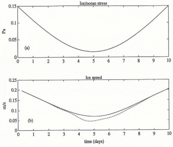
Fig. 1. (a) Specified total stress (including turbulent arid internal-mave stress) at the ice/ocean interface; (b) corresponding ice-drift speed for case 1, without internal wave dray (solid for all figures) and case 2, witli internal wave drag (dashed for all figures). Scalar fields shown in Figures 1 through 4 have been smoothed with a four-point (1 d) running average.

an expanding stack. In this way, the retreat of the mixed layer as ice melts can be followed closely despite a fairly coarse vertical grid. Entrainment reverses the process, working successively through the remanent mixed layers until the last is removed from the stack.

Two different model runs were made: one in which the ice under-surface was given a small-scale roughness length of 2 cm, but is otherwise smooth; and a second, with the same value for z ₀, but with large-scale relief with

Fig. 2. (a) Effective drag coefficient, (b) Magnitude of the angle between interfacial stress and surface (ice) velocity.

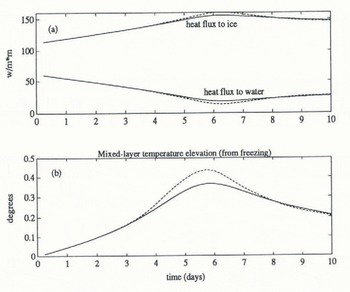
Fig. 3. (a) Heat flux to the ice (i.e. bottom melting) and to the mixed layer. (b) Difference between mixed-layer temperature and mixed-layer freezing temperature. The model is initially at freezing.

k ₀ = 0.063m⁻¹ and h ₀ = 1.4 (McPhee and Kantha, 1989) in order to assess the impact of the internal wave model.

Figures 1 and 2 show the response of ice drift. Early on, the mixed layer is deep and the drag coefficients are similar. As the wind dies, meltwater begins to accumulate nearer the surface and the resulting stratification affects the drift response in dramatically different ways: for the case with no internal wave drag, there is a slight decrease in the magnitude of the drag coefficient and a substantial increase in the turning angle, i.e. the angle between interfacial stress and surface-drift velocity. With large-scale underside relief, momentum is transferred directly into the internal wave-field, so that drag increases by a large factor and the turning angle decreases. As the wind picks up in the second half of the period, the mixed layer deepens (Fig. 4a), lessening

Fig. 4. (a) Mixed-layer depth. (b) Mixed-layer salinity.

Fig. 5. Density (−1000) profiles for successive days. Triangles show grid-point values for case 1, while the solid and dashed curves show step structure retained by the “remanent mixed-layer” stack. Note that density remains unchanged at the bottom, four grid paints.

momentum loss to internal waves, and eventually the ice gains enough speed to outrun its internal wake.

Thermodynamics is summarized in Figure 3. Most of the heat flux introduced at the interface melts ice (150 W m⁻² is roughly equivalent to 5 cm d⁻¹ ice melt), but note that, in the first few days, a substantial proportion goes to heating the mixed layer (Fig. 3b).

Mixed-layer salinity (Fig. 4b) decreases overall in response to the influx of fresh meltwater at the surface, but increases from a minimum on day 6 as turbulent entrainment is forced by the increasing surface stress. A more detailed view of the density structure is provided by Figure 5, showing daily density (−1000) profiles in succession. The symbols denote values at grid points, but the intermediate step-structure associated with the remanent mixed layers is also shown. By the end of the period, all of the remanent mixed layers have been entrained.

Summary

A quasi-analytical upper-ocean model has been developed for describing fluxes of momentum, heat and salt at the ice/ocean interface, and within the mixed-layer/upper pycnocline system. The model incorporates ideas suggested by recent observational studies, including a realistic model for heat and mass transfer at the ice/ocean boundary, and a treatment of momentum flux lost from the ice/upper-ocean system in the internal wave-field.

The turbulence model provides a detailed account of velocity and Reynolds stress structure in the turbulent boundary layer and, as such, is considerably more complex than most “slab” type mixed-layer models (e.g. Houssais, Reference Houssais1988). Nevertheless, it can be used in a model of upper-ocean temperature and salinity with relatively coarse vertical and time resolution.

Acknowledgements

Support for this work by the Office of Naval Research, through Contract N00014-84-C-0028, and by the National Science Foundation, through Grant OCE-8923072, is gratefully acknowledged.