


1. Introduction
Similitude is one of the few properties of turbulence that makes understanding the phenomenon more tractable. This principle is indeed the basis for much of turbulence theory (Reynolds Reference Reynolds1883; von Kármán Reference von Kármán1930; Kolmogorov Reference Kolmogorov1941; Townsend Reference Townsend1976). The challenge, of course, is to identify the appropriate similitude (scaling) parameter for a given feature. In boundary layer research, scaling analyses have led to considerable success in characterizing the size and intensity of coherent turbulent structures (McKeon & Sreenivasan Reference McKeon and Sreenivasan2007; Klewicki Reference Klewicki2010; Marusic et al. Reference Marusic, McKeon, Monkewitz, Nagib, Smits and Sreenivasan2010; Smits, McKeon & Marusic Reference Smits, McKeon and Marusic2011; Jiménez Reference Jiménez2018). Scaling becomes particularly important for flows with high Reynolds numbers which exhibit a wider range of turbulent motions due to the increased separation between the smallest and largest scales. The friction Reynolds number  ${Re}_\tau \equiv {u_\tau } \delta / \nu$ quantifies the difference between the boundary layer thickness $\delta$ limiting the largest motions and the viscous length $\nu / {u_\tau }$ describing the near-wall features. Here, $\nu$ is the kinematic viscosity and ${u_\tau }$ is the friction velocity corresponding to the average wall shear stress.
In recent decades, the predominant focus for studies of boundary layer structures in the logarithmic (log) region has been on larger-scale, energy-containing motions (see, e.g. Marusic et al. Reference Marusic, McKeon, Monkewitz, Nagib, Smits and Sreenivasan2010; Smits et al. Reference Smits, McKeon and Marusic2011). In the present context, these features include both  $O(\delta )$ very-large-scale motions (Kim & Adrian Reference Kim and Adrian1999; Guala, Hommema & Adrian Reference Guala, Hommema and Adrian2006; Hutchins & Marusic Reference Hutchins and Marusic2007) and $O(z)$ ‘attached’ or wall-coherent structures in accordance with Townsend's attached eddy hypothesis (Townsend Reference Townsend1976, p. 152), where $z$ is the wall-normal distance (see, e.g. Agostini & Leschziner Reference Agostini and Leschziner2017; Lozano-Durán & Bae Reference Lozano-Durán and Bae2019; Eich et al. Reference Eich, de Silva, Marusic and Kähler2020). While there have been numerous studies on smaller-scale vortices in the context of larger-scale features such as hairpin-type packets and vortex clusters (e.g. Adrian, Meinhart & Tomkins Reference Adrian, Meinhart and Tomkins2000b; Ganapathisubramani, Longmire & Marusic Reference Ganapathisubramani, Longmire and Marusic2003; del Álamo et al. Reference del Álamo, Jiménez, Zandonade and Moser2006; Wu & Christensen Reference Wu and Christensen2006), detailed analyses of the vortex core size in boundary layer turbulence are fewer. The existing results have consistently shown the most probable vortex core diameter to be near 10 $\eta$ (Tanahashi et al. Reference Tanahashi, Kang, Miyamoto, Shiokawa and Miyauchi2004; Herpin, Stanislas & Soria Reference Herpin, Stanislas and Soria2010; Herpin et al. Reference Herpin, Stanislas, Foucaut and Coudert2013; Wei et al. Reference Wei, Elsinga, Brethouwer, Schlatter and Johansson2014), where $\eta$ is the Kolmogorov length scale. The moderate discrepancy in detected size across the cited studies may be due to variations in methodology, which will be discussed further in the analysis. The characteristic velocity for the vortex, i.e. the maximum azimuthal velocity around the vortex centre, has yielded more mixed results. Tanahashi et al. (Reference Tanahashi, Kang, Miyamoto, Shiokawa and Miyauchi2004) argued for scaling by the Kolmogorov velocity $u_\eta$ despite observing moderate increase with increasing Reynolds number, and Wei et al. (Reference Wei, Elsinga, Brethouwer, Schlatter and Johansson2014) suggested a mixed scaling of $u_\eta$ and $u{{}^{\prime }}$ which is the streamwise root-mean-square (r.m.s.) velocity. The more consistent finding across studies relates to the vortex position which is less susceptible to methodology bias: the small-scale vortices are intermittently distributed and clustered in space (del Álamo et al. Reference del Álamo, Jiménez, Zandonade and Moser2006; Wu & Christensen Reference Wu and Christensen2006; Kang, Tanahashi & Miyauchi Reference Kang, Tanahashi and Miyauchi2007; Jiménez Reference Jiménez2013).
The observed clustering of vortices is consistent with the apparent self-organization of the instantaneous flow in high-Reynolds-number boundary layers into large-scale velocity structures separated by relatively thin layers of concentrated shear and vorticity (Meinhart & Adrian Reference Meinhart and Adrian1995; Priyadarshana et al. Reference Priyadarshana, Klewicki, Treat and Foss2007; Eisma et al. Reference Eisma, Westerweel, Ooms and Elsinga2015; de Silva et al. Reference de Silva, Philip, Hutchins and Marusic2017). These thin layers are referred to here as internal shear layers (ISLs). A majority of the prograde spanwise vortex cores reside along these shear layers (Heisel et al. Reference Heisel, Dasari, Liu, Hong, Coletti and Guala2018), where prograde here indicates rotation direction consistent with the mean shear. Recent studies on ISLs have indicated robust scaling behaviour. The layer thickness is proportional to the Taylor microscale  $\lambda _T$ (Wei et al. Reference Wei, Elsinga, Brethouwer, Schlatter and Johansson2014; Eisma et al. Reference Eisma, Westerweel, Ooms and Elsinga2015; de Silva et al. Reference de Silva, Philip, Hutchins and Marusic2017) or $\delta {Re}_\tau ^{-1/2}$ (Morris et al. Reference Morris, Stolpa, Slaboch and Klewicki2007; Klewicki Reference Klewicki2013), and the streamwise velocity difference across the layer is proportional to ${u_\tau }$ (de Silva et al. Reference de Silva, Philip, Hutchins and Marusic2017; Heisel et al. Reference Heisel, Dasari, Liu, Hong, Coletti and Guala2018, Reference Heisel, de Silva, Hutchins, Marusic and Guala2020b; Gul, Elsinga & Westerweel Reference Gul, Elsinga and Westerweel2020).
The velocity structures separated by the ISLs are often identified using a general classification known as the uniform momentum zone (UMZ), a region with relatively uniform streamwise velocity (Meinhart & Adrian Reference Meinhart and Adrian1995). A UMZ is uniform relative to the surrounding flow such that low-amplitude turbulent fluctuations within the zone can be neglected. UMZs are detected using histograms of the streamwise velocity (Adrian et al. Reference Adrian, Meinhart and Tomkins2000b) or fuzzy clustering (Fan et al. Reference Fan, Xu, Yao and Hickey2019), often with two-dimensional flow fields in the streamwise–wall-normal ( $x$–
$x$– $z$) plane from imaging experiments (de Silva, Hutchins & Marusic Reference de Silva, Hutchins and Marusic2016; Saxton-Fox & McKeon Reference Saxton-Fox and McKeon2017; Laskari et al. Reference Laskari, de Kat, Hearst and Ganapathisubramani2018), including in atmospheric turbulence (Morris et al. Reference Morris, Stolpa, Slaboch and Klewicki2007; Heisel et al. Reference Heisel, Dasari, Liu, Hong, Coletti and Guala2018). Because of their generic definition, detected UMZs are likely to be associated with other coherent velocity structures such as elongated ‘streaky’ structures (Hwang Reference Hwang2015), large-scale sweep events (Laskari et al. Reference Laskari, de Kat, Hearst and Ganapathisubramani2018) and travelling waves (Saxton-Fox & McKeon Reference Saxton-Fox and McKeon2017; Laskari & McKeon Reference Laskari and McKeon2021). A favourable aspect of the UMZ classification, compared with methods that detect and extract specific velocity structures localized in space, is that it allows for a systematic quantification of how the coherent velocity structures are organized throughout the boundary layer for a given measured realization of the flow. Heisel et al. (Reference Heisel, de Silva, Hutchins, Marusic and Guala2020b) compared the UMZ properties across a wide range of Reynolds number and surface roughness to demonstrate that the organization of zones universally exhibits the theoretical scaling behaviour of the log region, i.e. size and velocity proportional to wall-normal distance and friction velocity, respectively. The findings are consistent with previous studies that showed wall-normal distance scaling of more specific isolated velocity structures such as the attached streaky structures (e.g. Hwang Reference Hwang2015; Hwang & Sung Reference Hwang and Sung2018) and streamwise rolls (e.g. del Álamo et al. Reference del Álamo, Jiménez, Zandonade and Moser2006; Lozano-Durán, Flores & Jiménez Reference Lozano-Durán, Flores and Jiménez2012; Jiménez Reference Jiménez2018).
The general self-organization of structures described above is qualitatively similar to findings in isotropic turbulence research. Specifically, shear and vortex structures are known to cluster spatially (She, Jackson & Orszag Reference She, Jackson and Orszag1990; Moisy & Jiménez Reference Moisy and Jiménez2004). The characteristic length of the vortex tubes and the cluster is proportional to the integral length scale  $L$ (Jiménez et al. Reference Jiménez, Wray, Saffman and Rogallo1993; Ishihara, Gotoh & Kaneda Reference Ishihara, Gotoh and Kaneda2009), as is the distance between clusters (Ishihara, Kaneda & Hunt Reference Ishihara, Kaneda and Hunt2013). The intense vortex tubes primarily reside within thin shear layers whose thickness is again proportional to $\lambda _T$ (Ishihara et al. Reference Ishihara, Kaneda and Hunt2013; Elsinga et al. Reference Elsinga, Ishihara, Goudar, da Silva and Hunt2017). The observations are consistent with an earlier prediction by Saffman (Reference Saffman1968) that large-scale vortex sheets have thickness of order $\lambda _T$. Based on the recent findings, the organization of clustered vortex tubes into intermittent shear layers has been proposed as an important component of small-scale dynamics (Elsinga & Marusic Reference Elsinga and Marusic2010; Hunt et al. Reference Hunt, Eames, Westerweel, Davidson, Voropayev, Fernando and Braza2010; Ishihara et al. Reference Ishihara, Kaneda and Hunt2013; Hunt et al. Reference Hunt, Ishihara, Worth and Kaneda2014; Elsinga et al. Reference Elsinga, Ishihara, Goudar, da Silva and Hunt2017). The organization is consistent with intermittency principles, where the clustering of strong velocity gradients leads to heavy-tailed probability distributions which influence high-order statistics (She & Leveque Reference She and Leveque1994; Sreenivasan & Antonia Reference Sreenivasan and Antonia1997). Despite the matched scaling and common features, there are key differences between the isotropic and boundary layer organizations. Most notably in the boundary layer case, the presence of the mean shear leads to a preferential direction and persistence of the coherent structures and significant large-scale anisotropy. Nevertheless, there is reason to be cautiously optimistic. If the behaviour of the shear layers has universal properties, it could provide a structural representation for scale interaction and the energy cascade.
In addition to the limited number of detailed studies on vortex cores and ISLs in high-Reynolds-number boundary layer turbulence, even fewer works have quantitatively explored possible relations between the coherent velocity structures, vortices and shear layers. Accordingly, the properties of both prograde spanwise vortices and internal shear layers are explored here in a single comparative analysis. The goal is to identify similarities in the behaviour of these features, and to better understand their dynamical relationship with the local larger-scale coherent velocity structures. Particular attention is paid to why the Taylor microscale is a relevant similarity parameter for these features in high-Reynolds-number turbulence.
The behaviour of ISLs is inferred here based on the properties of detected UMZ interfaces. For the vortex cores, the analysis is focused on prograde vortices due to their closer connection with the predominately positive shear layers (i.e.  $\partial u / \partial z>$ 0) that populate the boundary layer. Both analyses are conducted in the streamwise–wall-normal plane using the same suite of particle image velocimetry (PIV) experiments as in Heisel et al. (Reference Heisel, de Silva, Hutchins, Marusic and Guala2020b), which spans a wide range of Reynolds number and surface roughness and includes a field experiment in the atmospheric surface layer (ASL, Heisel et al. Reference Heisel, Dasari, Liu, Hong, Coletti and Guala2018). The remainder of the article is organized into the following sections: the experiments and methodology are described in § 2; results on the vortex and shear layer size (§ 3) and velocity (§ 4) are then presented; our interpretation of the results are reserved for the discussion in § 5; the article concludes with a summary in § 6. Two appendices are included to examine the influence of spatial resolution on the results and to justify assumptions made in the analysis.
1.1. Terminology
In this work, the outer layer of the boundary layer begins above the buffer layer (for smooth surfaces) or roughness sublayer (rough surfaces), and consists of the log and wake regions. The term ‘small-scale’ refers to the smallest turbulent eddies proportional to the Kolmogorov length  $\eta$ and velocity $u_\eta$. The term ‘large-scale’ refers to the streamwise integral length $L$ and r.m.s. velocity $u{{}^{\prime }}$. In this context, the Taylor microscale is then an intermediate length scale $\lambda _T \sim \eta ^{2/3}L^{1/3}$ (Pope Reference Pope2000), where ‘ $\sim$’ means ‘scales with’. The term ‘vortex core’ is used here to differentiate the detected strongly rotating vortices from larger-scale, diffuse vortical motions such as rolls and bulges. The estimated probability density function (p.d.f.) of any variable ‘ $s$’ is given the notation $p_s$. Unless otherwise noted, lowercase lettering is used for instantaneous values of a variable, and uppercase lettering is used for the average of the same variable. Angled brackets ‘ $\langle \cdot \rangle$’ are also used to indicate ensemble averages. Bold typeface is used for variables that are vectors. The superscript ‘ $+$’ indicates normalization in wall units, i.e. $z^{+} = z {u_\tau } / \nu$ and $u^{+} = u/{u_\tau }$. The subscript ‘ $\omega$’ is used for variables corresponding to vortex properties. The subscript ‘ $i$’ is used for variables corresponding to ISL properties. Finally, as stated above, the coordinate system employed here uses $z$ (
$z$ ( $w$) for the wall-normal direction (velocity).
2. Methodology
2.1. Experiments
Nine flow cases covering several orders of magnitude in Reynolds number  ${Re}_\tau \sim O(10^{3}-10^{6})$ and surface roughness $k_s^{+} \lesssim O(10^{4})$ are included in the present analysis. Here, $k_s$ is the equivalent sand-grain roughness and conditions are fully rough for $k_s^{+} \gtrsim$ 70 when the surface drag becomes independent of viscosity. The flow cases, previously used together in Heisel et al. (Reference Heisel, de Silva, Hutchins, Marusic and Guala2020b), are summarized in table 1. An overview of important details is given here, and a full account of each experiment is available from the cited references in the table.
Table 1. Experimental datasets used in the analysis of prograde spanwise vortices and ISLs.

The direct numerical simulation (DNS) of a boundary layer with  ${Re}_\tau = 2000$ by Sillero et al. (Reference Sillero, Jiménez and Moser2013) is included for comparison with the experimental cases. The DNS case was analysed using two-dimensional flow fields in the $x$–
$x$– $z$ plane to be consistent with the PIV experiments. The variable $\Delta x$, representing the spatial resolution, refers to the streamwise grid spacing for the DNS and the vector field spacing for the PIV experiments, which all employed 50 % window overlap leading to interrogation window size 2 $\Delta x$. The parameters $\eta$ and $\lambda _T$ are both dependent on wall-normal distance $z$. The normalized resolution in table 1 considers the average parameter values at $z=0.1\delta$. This reference position was chosen in terms of $\delta$ because later results are presented at matched $z/\delta$ in the outer layer. Determination of $\eta$ and $\lambda _T$ is detailed in § 2.2.
The HRNBLWT facility in table 1 refers to the High Reynolds Number Boundary Layer Wind Tunnel at the University of Melbourne. The flow cases corresponding to the HRNBLWT were measured using the high-resolution tower PIV configuration detailed in Squire et al. (Reference Squire, Morrill-Winter, Hutchins, Marusic, Schultz and Klewicki2016). The sandpaper roughness flow cases from the same study are not included in the present analysis. In this case a higher degree of small-scale noise in the rough-wall measurements (as documented in Squire et al. Reference Squire, Morrill-Winter, Hutchins, Marusic, Schultz and Klewicki2016) precludes the possibility of accurately fitting the Oseen vortex model to extract vortex statistics, and hence these data are omitted from the present study.
The SAFL facility in table 1 is the boundary layer wind tunnel at St. Anthony Falls Laboratory, University of Minnesota. These measurements captured the bottom portion of the boundary layer thickness, including the log region and part of the wake region. For the mesh roughness cases, the tunnel floor was covered by woven wire mesh with 3 mm wire diameter and 25 mm opening size (Heisel et al. Reference Heisel, de Silva, Hutchins, Marusic and Guala2020b).
The ASL measurements were acquired using super-large-scale PIV (SLPIV) in the lowest 20 m of the atmosphere with natural snowfall as the flow tracers. The measurements captured the roughness sublayer and bottom of the log region in near-neutral conditions at the Eolos field facility. A detailed discussion of the snowflake traceability is given in Heisel et al. (Reference Heisel, Dasari, Liu, Hong, Coletti and Guala2018). The SLPIV method cannot capture the smallest vortical motions in the ASL due to both the non-negligible snowflake inertia and the coarse spatial resolution relative to  $\eta$. Yet numerous vortices were present in each SLPIV vector field with size $O$(1 m) likely augmented by coarse resolution. The vortex and ISL size statistics are included in this study, but caution must be taken in interpreting these results. Vortex and shear layer velocity statistics in the ASL, however, are shown to be in agreement with all laboratory-scale trends.
Profiles of the first- and second-order velocity statistics are shown for each flow case in figure 1. For two of the smooth-wall cases ( $\times ,+$), the relatively lower wall-normal velocity statistics in figure 1(c,d) are attributed to measurement resolution as discussed in Heisel et al. (Reference Heisel, Katul, Chamecki and Guala2020a). The decreasing trends in figure 1(c,d) for the ASL case ( $\bullet$) may be due to one or more of several challenges present in atmospheric field settings. For instance, uncertainty in the definition of $\delta$, statistical convergence of higher-order statistics, and the possible role of large-scale stratified motions at higher altitudes are all discussed in the original study (Heisel et al. Reference Heisel, Dasari, Liu, Hong, Coletti and Guala2018).

Figure 1. First- and second-order velocity statistics for each experimental dataset. (a) Mean streamwise velocity  $U$ shown as a deficit from the free-stream condition $U_\infty$, where $\kappa ^{-1}$ is the logarithmic slope based on the von Kármán constant. (b) Streamwise variance $\langle u^{2} \rangle$. (c) Wall-normal variance $\langle w^{2} \rangle$. (d) Reynolds shear stress $-\langle u w \rangle$. Profiles are normalized by the friction velocity ${u_\tau }$ and boundary layer thickness $\delta$. Data symbols correspond to the experiments in table 1 and are shown with logarithmic spacing for clarity. The roughness sublayer is excluded from the ASL profiles.
2.2. Scaling parameters
Owing to their importance in the scaling analysis, the determination of relevant flow parameters is discussed here. Not included here is  ${u_\tau }$, which is discussed in the original publications cited in table 1. For the wind tunnel studies (HRNBLWT and SAFL), the parameters were estimated using hot-wire anemometer measurements under the same flow conditions rather than the PIV measurements (Squire et al. Reference Squire, Morrill-Winter, Hutchins, Marusic, Schultz and Klewicki2016; Heisel et al. Reference Heisel, de Silva, Hutchins, Marusic and Guala2020b). Parameter estimation for the ASL case relied on scaling assumptions which are discussed separately at the end of this section.
Many of the parameters depend on the average rate of turbulent energy dissipation  $\epsilon$. The Kolmogorov scales are defined as the length $\eta \equiv (\nu ^{3}/\epsilon )^{1/4}$, velocity $u_\eta \equiv (\nu \epsilon )^{1/4}$ and time $\tau _\eta \equiv (\nu / \epsilon )^{1/2}$. Further, the definition used here for the streamwise integral length is $L = {u{{}^{\prime }}}^{3} / \epsilon$ and for the large-eddy turnover time is $T = {u{{}^{\prime }}}^{2} / \epsilon$. This integral length definition yields results similar to the autocorrelation method, based on a test using the hot-wire measurements. The turnover time $T$ is equivalent to the integral time scale definition in isotropic turbulence where $T = L / u{{}^{\prime }}$, and differs from the streamwise integral time in wall-bounded flows where $T_{int} = L/U$.
Because  $\epsilon$ could not be measured directly, various estimation methods were used depending on the experiment. Dissipation was estimated as $\epsilon \approx 15 \nu \langle (\partial u / \partial x )^{2} \rangle$ assuming local isotropy with the HRNBLWT measurements (Squire et al. Reference Squire, Morrill-Winter, Hutchins, Marusic, Schultz and Klewicki2016). For the DNS and SAFL cases, the dissipation was inferred from the value of the longitudinal second-order structure function in the inertial subrange, i.e. $D_{11} = C \epsilon ^{2/3} r^{2/3}$ (Saddoughi & Veeravalli Reference Saddoughi and Veeravalli1994).
The Taylor microscale is defined here as  $\lambda _T^{2} = {u{{}^{\prime }}}^{2} / \langle (\partial u / \partial x )^{2} \rangle$ and the value was estimated using this expression for all cases excluding the ASL. This definition is specific to the streamwise component, where the Taylor microscale is anisotropic in wall-bounded turbulence (Morishita, Ishihara & Kaneda Reference Morishita, Ishihara and Kaneda2019). The Taylor microscale and integral length are related as $\lambda _T / L \sim {Re}_L^{-1/2}$ with the integral Reynolds number being ${Re}_L = u{{}^{\prime }}L / \nu$ (Pope Reference Pope2000). This relationship is based on $\epsilon \sim \nu \langle (\partial u / \partial x )^{2} \rangle$, where the proportional constant is 15 for isotropic turbulence and otherwise depends on the relative contribution of each gradient term to the dissipation.
For the ASL case, the measurement resolution of both the SLPIV and a collocated sonic anemometer were too coarse for the estimation methods discussed above. The dissipation was therefore estimated as  $\epsilon \approx {u_\tau }^{3} / \kappa z$, where $\kappa$ is the von Kármán constant. This estimate assumes the local shear production of turbulence in the log region is in equilibrium with the dissipation rate, which is typical for high-Reynolds-number boundary layers (Townsend Reference Townsend1961). The Kolmogorov length scale resulting from this approximation is $\eta \approx 0.7\pm 0.2$ mm. The value for $\lambda _T$ was estimated from the expression $\epsilon = 15 \nu {u{{}^{\prime }}}^{2} / \lambda _T^{2}$, which assumes local isotropy and combines the $\lambda _T$ and $\epsilon$ expressions through the shared gradient term. The resulting Taylor microscale estimate for the ASL case is $\lambda _T \approx 13$ cm. The integral length $L \sim O$(1 m) results directly from the estimated dissipation.
2.3. Spanwise vortex detection
Numerous methods exist to characterize vortices (see, e.g. Chakraborty, Balachandar & Adrian Reference Chakraborty, Balachandar and Adrian2005; Haller Reference Haller2005). The preferred method in the present analysis is to fit the local flow field to a model vortex. The primary advantage of using a model vortex is that the fitted vortex properties are not dependent on an arbitrary parameter threshold. However, a parameter threshold is still required to detect the possible vortex core regions upon which the model is fitted, and the characterization of complex vortex structures is limited to the imposed model shape. Despite these limitations, recent studies have successfully characterized large populations of vortex cores in boundary layer flows using the Oseen model (Oseen Reference Oseen1912) in cylindrical coordinates (Carlier & Stanislas Reference Carlier and Stanislas2005; Herpin et al. Reference Herpin, Stanislas and Soria2010, Reference Herpin, Stanislas, Foucaut and Coudert2013)
 \begin{equation} \boldsymbol{u} = \boldsymbol{u}{_\omega} + \frac{\varGamma}{2 {\rm \pi}r} \left[ 1 - \exp \left( - \left( \frac{ r }{ r{_\omega}} \right) ^{2} \right) \right] \boldsymbol{e}_{\theta},\end{equation}
where  $\boldsymbol {u}{_\omega }$ is the advection velocity of the vortex, $\varGamma$ is the circulation, $r$ is the radial distance from the vortex centre, $r{_\omega }$ is the vortex radius and $\boldsymbol {e}_{\theta }$ is the unit vector in the azimuthal direction. The model incorporates Biot–Savart law for the velocity induced by a vortex line, i.e. $u_\theta \propto \varGamma / 2 {\rm \pi}r$, and the exponential term acts as a damping function to decrease the azimuthal velocity $u_\theta$ inside the vortex radius such that the maximum velocity occurs at $r=r{_\omega }$.
The Oseen model is consistent with the Navier–Stokes equations in its three-dimensional definition. In the formal definition, the radius is given as  $r{_\omega } = \sqrt {4\nu t}$, where the radius is zero at time $t=0$ and the vortex grows in time via viscous diffusion. This is conceptually different from the Burgers vortex radius $r{_\omega } = \sqrt {4\nu / \alpha }$, where $\alpha$ is the strain rate. Rather than growing in time, the Burgers vortex size is steady due to a balance between outward diffusion and an inward radial velocity $u_r(r) = -\alpha r$ induced by axial vortex stretching (Burgers Reference Burgers1948). The Oseen model does not include a radial velocity or axial stretching. This distinction between the two models becomes important for interpreting the later results.
The vortex detection using (2.1) followed the procedure of Herpin et al. (Reference Herpin, Stanislas, Foucaut and Coudert2013), which is briefly summarized here. Possible vortex cores were identified based on flow regions with  $\lambda _{ci} > 1.5 \lambda _{rms}$, where $\lambda _{ci}$ is the two-dimensional swirling strength (Adrian, Christensen & Liu Reference Adrian, Christensen and Liu2000a) and $\lambda _{rms}(z)$ is the r.m.s. swirling strength at each wall-normal distance. The threshold introduces selection bias on the vortices, but the threshold is not applied in the later model fit. Based on a test using one flow case, changing the threshold factor from 1.5 $\times$ to 2 $\times$ or 2.5 $\times$ resulted in the detection of fewer vortices, but resulted in no statistically significant changes to the vortex properties.
A notable deviation to the original procedure was to apply a Gaussian filter to the wind tunnel (HRNBLWT and SAFL) PIV fields prior to vortex detection. The filter removed small-scale noise in the gradients which significantly improved the performance of the fitting algorithm. The size of the Gaussian filter, i.e. its standard deviation, was selected to be approximately 2 $\eta$ for the reference position $z=0.1\delta$ in each case. The filter was not applied to the DNS or SLPIV vector fields. The filter would be negligibly small relative to the resolution for the ASL case, and a comparison of DNS results with and without the filter revealed no changes to the statistics of interest.
The properties of the identified core region were used as initial guesses for the six vortex model parameters: the centre position given by  $x{_\omega }$ and $z{_\omega }$, the advection velocity components $u{_\omega }$ and $w{_\omega }$, the circulation $\varGamma$ and the radius $r{_\omega }$. The initial value for $\varGamma$ was based on the core area and average out-of-plane vorticity $\omega _y$ within the core region. The initial guesses for $r{_\omega }$, $x{_\omega }$ and $z{_\omega }$ were used to extract the local vector field within 2 $r{_\omega }$ of the vortex centre. The extracted vector field was then fitted to (2.1) using the initial guesses and a nonlinear least-squares fitting algorithm. The algorithm was designed to update the six model parameters until the difference between the local vector field and the model vortex (i.e. the right-hand side of (2.1)) was minimized. The parameters output by the algorithm therefore describe the model vortex most closely matching the vector field within and around the vortex core. The parameters are thus inferred to represent the vortex core properties. The initial guesses informed by the detected core regions reduce the likelihood the algorithm diverged to a spurious local minimum in the model parameter space. To exclude these fits and other ill-fitted results, the properties are only considered for vortices where the coefficient of determination exceeded $R^{2}> 0.6$. Increasing the imposed minimum $R^{2}$ value reduces somewhat the convergence of the vortex statistics, but does not change the overall trends and conclusions of the study. An example vector field and closest model fit with
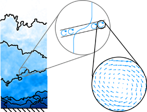
  $R^{2}= 0.9$ are shown in figure 2(a).

Figure 2. Example of a model Oseen vortex fitted to a velocity vector field, shown with the vortex advection velocity subtracted for visualization. (a) Comparison of measured velocities (black vectors) relative to the closest Oseen model (red vectors) whose size is given by the red circle. (b) Notation for the diameter  $d{_\omega }$ and azimuthal velocity difference $\Delta u{_\omega }$ across the diameter of the fitted vortex.
Besides the advection velocity, the characteristic velocity of each vortex is the maximum azimuthal velocity difference  $\Delta u{_\omega }$ across the vortex. This velocity, shown in figure 2(b), is twice the azimuthal velocity at the edge of the vortex $r=r{_\omega }$ due to axisymmetry and the definition of the radius. From (2.1), the velocity is
 \begin{equation} \Delta u{_\omega} = \frac{\varGamma}{{\rm \pi} r{_\omega}} ( 1 - e^{{-}1} ).\end{equation}
The properties are defined across both sides of the vortex core, i.e. as  $d{_\omega }$ and $\Delta u{_\omega }$, for comparison with the ISL properties which are not in cylindrical coordinates.
The detection algorithm was conducted for all experimental datasets in table 1. Approximately 22 000 Oseen vortices were fitted for the ASL dataset, and more than 100 000 were fitted for every other case. The possible issue of selection bias due to the chosen vortex model is discussed later in § 5.3. The primary sources of uncertainty for vortex properties in the PIV experiments are spatial resolution limitations and small-scale noise. The results are focused on probability distributions of the properties rather than their mean. Artefacts due to the limitations described above occur primarily within the smallest values of each property, and conclusions are not drawn from these regions of the distributions. See Appendix A for an assessment of how measurement resolution affects the mode and tail of the probability distributions. A further benefit of a probabilistic approach is to identify the possible relevance of multiple scaling parameters. If different regions of the probability distribution are governed by separate parameters, the mean value may not reflect a simple scaling relationship. A similar probability analysis of the ISL features is unfortunately not possible for the methodology given in the following section. The analysis requires conditionally averaging which does not provide instantaneous statistics.
2.4. ISL detection
Rather than directly detecting the ISLs using a threshold on instantaneous values of  $\partial u / \partial z$, we instead infer the properties of ISLs from detected interfaces of UMZs. These interfaces represent the shear regions separating the local larger-scale coherent velocity structures (de Silva et al. Reference de Silva, Philip, Hutchins and Marusic2017). In the present context, the distinction between ISLs and UMZ interfaces is largely a matter of detection methodology. While the shear layers align closely with UMZ interfaces, the interfaces can also include segments where the instantaneous shear is relatively smaller (Gul et al. Reference Gul, Elsinga and Westerweel2020). These additional segments due to the detection methodology may lead to differences between ISL and UMZ interface statistics for some properties. However, the statistics presented here are limited to those where the same behaviour has been previously reported for both ISLs and UMZ interfaces, and from here on the ISL terminology is applied.
The present analysis uses the same detected UMZs from Heisel et al. (Reference Heisel, de Silva, Hutchins, Marusic and Guala2020b). The methodology to identify UMZs and their interfaces using histograms of the streamwise velocity is detailed in the previous work. An important consideration regarding the previous study is that the detected UMZs unambiguously exhibited a dependence on wall-normal distance  $z$ (Heisel et al. Reference Heisel, de Silva, Hutchins, Marusic and Guala2020b), such that the present analysis studies the shear layers separating $z$-scaled velocity structures.
Figure 3 shows an example of ISLs and their statistics based on measurements from the  ${Re}_\tau =17\ 000$ smooth-wall case in table 1. The PIV field in figure 3(a) illustrates the general, approximate organization of the streamwise velocity in the outer layer into relatively uniform regions (i.e. UMZs) separated by thin shear layers (black lines). The field in figure 3(b) is focused on the local vicinity of a single ISL to demonstrate the compiled statistics. The velocity difference between UMZs is a factor of ${u_\tau }$, and the velocity gradient occurs across a short distance centred around the wall-normal position $z_i$ of the ISL. The black dots in figure 3(b) represent the PIV vector positions near the ISL at the horizontal centre of the field. The PIV velocities were compiled at these vector positions to create a profile relative to the ISL position ( $z-z_i$) and velocity ( $u-u_i$ and $w-w_i$). These conditional profiles were compiled for every $x$ position of every ISL.

Figure 3. Example shear layers for the  ${Re}_\tau = 17\ 000$ smooth-wall case. (a) Streamwise velocity field from figure 2 of Heisel et al. (Reference Heisel, de Silva, Hutchins, Marusic and Guala2020b), with detected ISLs (black lines) and turbulent/non-turbulent interface (red line). (b) Velocity field in the vicinity of an ISL (black line) relative to the ISL position $z_i$ and velocity $u_i$. (c) Conditionally averaged velocity profile relative to the ISLs, indicating the average velocity difference $\Delta U_i$ and thickness $\delta {_\omega }$. The black box in the upper left of (a) indicates the size of the field in (b).
Averaging all the conditional streamwise profiles in the log region yields the profile in figure 3(c). As seen in the figure, the average velocity difference  $\Delta U_i$ results from linear fits to the profile above and below the ISL (de Silva et al. Reference de Silva, Philip, Hutchins and Marusic2017). One method for estimating the (vorticity) thickness $\delta {_\omega }$ is to assume the ISL is a mixing layer (Brown & Roshko Reference Brown and Roshko1974). Note the subscript ‘ $\omega$’ is used for the shear layer thickness $\delta {_\omega }$ to be consistent with notation in the literature. The mixing layer method uses the maximum velocity gradient within the layer $\partial \langle u-u_i \rangle / \partial z \vert _{max}$. The gradient is highest at the centre of the layer and quickly decreases away from the centre, such that the maximum gradient is not representative of the entire layer. In practice, the measured maximum gradient also depends strongly on the spacing of the grid points $\Delta x$ in the vicinity of the layer centre, and $\delta {_\omega }$ values from this method are a function of the measurement resolution.
The thickness  $\delta {_\omega }$ can more simply be estimated as the distance across which the velocity difference $\Delta U_i$ occurs (Eisma et al. Reference Eisma, Westerweel, Ooms and Elsinga2015). In addition to being less sensitive to measurement resolution, this estimate is more representative of the overall shear layer. This second method is used to calculate the thicknesses presented in later results. Note this method is still susceptible to resolution issues if the measurements are coarse relative to $\delta {_\omega }$, as is discussed later.
In many respects, it is important to distinguish the ISLs from the turbulent/non-turbulent interface (TNTI) separating the boundary layer flow from the free-stream condition (Elsinga & da Silva Reference Elsinga and da Silva2019), i.e. the red line in figure 3(a). Indeed, the TNTI was detected using a separate methodology based on the kinetic energy defect (Chauhan et al. Reference Chauhan, Philip, de Silva, Hutchins and Marusic2014b) prior to detection of the UMZs and the internal layers (Heisel et al. Reference Heisel, de Silva, Hutchins, Marusic and Guala2020b). However, for the specific statistics analysed in the present study, the same scaling behaviour is expected for both ISLs and the TNTI. Previous studies have shown the TNTI to have thickness  $\delta {_\omega } \sim O(\lambda _T)$ and velocity $\Delta U \sim O({u_\tau })$ (Bisset, Hunt & Rogers Reference Bisset, Hunt and Rogers2002; da Silva & Taveira Reference da Silva and Taveira2010; Chauhan, Philip & Marusic Reference Chauhan, Philip and Marusic2014a; de Silva et al. Reference de Silva, Philip, Hutchins and Marusic2017), matching the ISL literature results discussed in the introduction. Later figures showing wall-normal profiles of shear layer properties include ISLs and TNTIs, such that both features contribute to values in the wake region.
3. Size statistics
3.1. Shear layer thickness
The streamwise velocity profile relative to the ISLs, shown previously in the figure 3(c) example, is compared for all flow cases in figure 4(a). The ASL measurement resolution exceeds the vertical axis limits and the profile is not visible. There is otherwise close agreement across cases with normalization by  $\lambda _T$ and ${u_\tau }$. A comparison of the profiles with alternative length scale normalizations, e.g. $\nu / {u_\tau }$ and $\eta$, is presented elsewhere (e.g. de Silva et al. Reference de Silva, Philip, Hutchins and Marusic2017).

Figure 4. Estimated average thickness  $\delta {_\omega }$ of ISLs normalized by $\lambda _T$. (a) Conditional average profile of streamwise velocity relative to ISLs in the log region. (b) Thickness $\delta {_\omega }$ as a function of measurement grid spacing $\Delta x$, noting the interrogation window size for the PIV cases is 2 $\Delta x$. (c) Wall-normal profile of $\delta {_\omega }$. Data symbols correspond to the experimental datasets in table 1.
The average ISL thickness was calculated from the conditional profiles following the methodology discussed in § 2.4. The effect of measurement resolution on the estimated thickness is demonstrated in figure 4(b). The thickness estimate is relatively invariant to resolution for grid spacing  $\Delta x \lesssim 0.1 \lambda _T$. The four SAFL PIV cases with $\Delta x \approx 0.1 \lambda _T$ have mean thickness approximately 25 % larger than the cases with smaller $\Delta x$, suggesting the effects of resolution may begin near this value. Assuming the $\lambda _T$ scaling extends to field conditions, the resolution of the ASL measurements is too coarse for an accurate estimate of the ISL thickness, and no conclusions are drawn from the $\delta {_\omega }$ value in the ASL case.
A wall-normal profile of  $\delta {_\omega }$ was constructed using conditional ISL statistics in binned intervals of $z/\delta$. The resulting profile in figure 4(c) suggests a fixed relationship between $\delta {_\omega }$ and $\lambda _T$ throughout the outer layer. The proportionality $\delta {_\omega } \approx (0.3 - 0.5)\lambda _T$ and its invariance with wall-normal position are both in close agreement with previous studies (Eisma et al. Reference Eisma, Westerweel, Ooms and Elsinga2015; de Silva et al. Reference de Silva, Philip, Hutchins and Marusic2017). Note that normalization of $\delta {_\omega }$ by $\delta {Re}_\tau ^{-1/2}$ collapses the profiles across experiments, but the thickness varies with $z$, i.e. the profiles are not flat. The local parameter $\lambda _T(z)$ is required to achieve the observed invariance of $\delta {_\omega }(z)$ with wall-normal position. The scatter between cases in figure 4(c) is entirely consistent with the resolution findings in figure 4(b): the cases with coarser resolution relative to $\lambda _T$ have profile values closer to 0.5 $\lambda _T$, and cases with higher resolution have profile values closer to 0.3 $\lambda _T$. A new finding from the present results is that significant laboratory-scale roughness (i.e. $k_s^{+} \approx$ 500) does not modify the relationship between $\delta {_\omega }$ and $\lambda _T$ beyond the uncertainty due to resolution, thus confirming the scaling is not limited to smooth-wall conditions. Ebner, Mehdi & Klewicki (Reference Ebner, Mehdi and Klewicki2016) proposed that large roughness may affect the thickness of the shear layers and the overall organization of UMZs. However, the required roughness in terms of $k_s/ \delta$ for this effect to occur may be too great to maintain outer layer similarity.
3.2. Vortex diameter
As discussed in § 2.3, the prograde spanwise vortex core statistics are presented here as probability distributions rather than averages. Specifically, statistics are given as p.d.f.s, which were estimated discretely as binned histograms with amplitude scaled to achieve area unity, i.e. probability of one within the parameter space. To improve the statistical convergence of the probability tails, logarithmic spacing was used for the histogram binning intervals. The proper normalization of the histogram as a p.d.f. is then achieved by dividing the value of each bin by its respective bin width and the total number of occurrences in the histogram. Logarithmic bin intervals were only used where the scale of the abscissa is logarithmic. Combined with the large number of detected vortices in each flow case, the logarithmic binning allows for observation of six orders of magnitude in probability.
The estimated p.d.f.s of prograde vortex core diameter  $p_d$ for each experimental dataset are shown in figure 5. The p.d.f.s are shown with $d{_\omega }$ normalized by both the Kolmogorov length $\eta$ (a) and the Taylor microscale $\lambda _T$ (c). Figure 5 includes vortex cores from the entire outer layer, including the logarithmic and wake regions. Prior to constructing the histograms, the fitted vortex diameters were individually normalized using the average parameters $\eta (z{_\omega })$ and $\lambda _T(z{_\omega })$ local to the vortex wall-normal position $z{_\omega }$. Later figures presenting vortex core statistics also feature contributions from throughout the outer layer and utilize the individual normalization described here. Note that limiting the statistics to vortex cores at a specific wall-normal position does not affect the figure trends or the conclusions of the study.

Figure 5. Probability distributions  $p_d$ of diameter for all prograde vortex cores in the outer layer of the boundary layer: (a) p.d.f. normalized by the Kolmogorov length scale $\eta$; (b) conditional p.d.f. $p_{d/\eta }^{*} = p_{d/\eta }(d{_\omega } \mid d{_\omega } > 40\eta )$; (c) p.d.f. normalized by the Taylor microscale $\lambda _T$; (d) conditional p.d.f. $p_{d/\lambda _T}^{*} = p_{d/\lambda _T}(d{_\omega } \mid d{_\omega } > \lambda _T)$. Comparison of results in the hatched regions of (a,c) is precluded by variability in measurement resolution across cases, including the ASL case shown in the insets. The conditional p.d.f.s in (b,d) are used to evaluate the distribution tail shape parameterized by the slope $m_d$. Data symbols correspond to the experimental datasets in table 1.
Previous studies have described the most probable vortex size, i.e. the distribution mode, in terms of  $\eta$. The mode for the DNS case in figure 5(a) is approximately 10 $\eta$, which is between the values (8–10) $\eta$ observed by Tanahashi et al. (Reference Tanahashi, Kang, Miyamoto, Shiokawa and Miyauchi2004) and (12–13) $\eta$ by Herpin et al. (Reference Herpin, Stanislas, Foucaut and Coudert2013). While the observed range (10–20) $\eta$ in the mode across the remaining cases in figure 5(a) may be physically meaningful, it may also be attributed to variability in measurement resolution. Appendix A demonstrates that coarsening the DNS grid to $\Delta x^{+}$ values similar to the experimental cases results in the same observed range in mode position. The cross-hatched lines in figure 5 illustrate the diameter range where a strict comparison across cases is precluded by the influence of measurement resolution on the experimental cases with coarser $\Delta x$. Additionally, while there is an orders-of-magnitude difference in detected vortex size for the ASL case in the insets of figure 5(a,c), the difference is consistent with the orders-of-magnitude increase in $\Delta x$ seen in table 1. We therefore draw no conclusions regarding either the distribution mode across cases or the detected size of ASL vortex cores.
Relative to the DNS case, some of the experimental results exhibit an increased number of vortices smaller than 10 $\eta$ in figure 5(a). This increased detection of small vortices is likely an artefact of residual measurement noise. While it is possible to further quantify and filter the noise (see, e.g. Foucaut, Carlier & Stanislas Reference Foucaut, Carlier and Stanislas2004), its effect is confined to the hatched region of figure 5 which is already subject to resolution bias and is excluded from further analysis.
Regarding the distribution shape, Herpin et al. (Reference Herpin, Stanislas, Foucaut and Coudert2013) showed that the size probability  $p_d$ approximately follows a log-normal distribution, except with a somewhat thicker tail than the log-normal case. The figure 5 distribution tails are consistent with these findings. The tails deviate from a purely log-normal distribution and instead approximate a power law. The distribution tails shown in figure 5(b,d) are conditional p.d.f.s, e.g. $p_{d/\eta }^{*}=p_{d/\eta }(d{_\omega } \mid d{_\omega } > 40\eta )$, which describe the probability given the diameter is above the threshold shown as a dashed line in figure 5(a,c). The conditional p.d.f. is equivalent to taking $p_d$ above the threshold and rescaling to achieve area unity under the tail region. The rescaling removes the statistical contribution of the small-diameter vortices – which are affected by spatial resolution and measurement noise – to the amplitude of the normalized distribution tails. Given that the tail shape is not affected by resolution (see Appendix A), the $p_d^{*}$ plots allow for an unbiased comparison across cases for a consistent range of diameters.
The power law shape of the distribution tail is given by  $p_d^{*} \propto d{_\omega } ^{-m_d}$. The collapse of the tails in figure 5(b,d) is due to a consistent slope $m_d \approx 6-7$ across cases, suggesting $m_d$ is independent of Reynolds number and the surface roughness geometries tested here. The slope is the same for the ASL case, and also does not vary with wall-normal position. The steepness of the slope $m_d \approx 6 - 7$ imposes an effective maximum value on the vortex core size, where the probability density decreases by orders of magnitude and becomes negligibly small across a narrow range of sizes. However, the relevant scaling parameter cannot be determined by the shape of the power law, as $m_d$ is independent of the normalization as seen in figure 5(b,d). In this regard, the diameter of the largest detected vortex cores may be $O(100\eta )$ as in figure 5(b) or $O(1 - 10\lambda _T)$ as in 5(d).
To discern the scaling parameter relevant to the largest vortex cores, the curvature of  $p_d$ in the region preceding the power law must be considered. Given the sensitivity of the small-diameter vortex statistics to the measurement resolution (Appendix A), it is not possible to separate a physical trend in the figure 5 $p_d$ curvature from the variability of resolution across the experiments studied here. These experimental factors can be avoided by focusing the analysis on the DNS flow case. Owing to the Reynolds dependence $\eta / \lambda _T \sim {Re}_L^{-1/4}$ where ${Re}_L= u{{}^{\prime }}L / \nu$, the $d{_\omega }$ statistics for the DNS case were grouped in intervals of ${Re}_L$ based on the local mean values for $u{{}^{\prime }}$ and L at the vortex position $z{_\omega }$.
Figure 6(a,b) shows distributions of  $d{_\omega }$ for eight intervals of ${Re}_L$ within the DNS case. Having already demonstrated the power law shape of the probability tail in figure 5, the abscissa is shown with linear scaling in figure 6(a,b) to highlight amplitude differences along the tail. With $\eta$ normalization, there is a clear Reynolds number trend in the distribution tail region corresponding to large diameter vortex cores. Normalization by $\lambda _T$ in figure 6(b) leads to improved agreement across the range of ${Re}_L$ represented. There is no apparent trend in Reynolds number along the tails of $p_{d/\lambda _T}$ and the remaining narrow scatter is attributed to incomplete statistical convergence.

Figure 6. Probability distributions of the vortex core diameter  $d{_\omega }$ and strain rate $\alpha = 16 \nu d{_\omega }^{-2}$ inferred from the Burgers vortex. Diameter p.d.f. $p_d$ normalized by (a) the Kolmogorov length scale $\eta$ and (b) the Taylor microscale $\lambda _T$. Strain rate p.d.f. $p_\alpha$ normalized by (c) the Kolmogorov time scale $\tau _\eta$ and (d) the large-eddy turnover time $T$. Data shown are for the DNS case in intervals of the integral Reynolds number ${Re}_L$ determined by the local flow properties at the wall-normal position of the vortex. The upper right plot shows a profile of ${Re}_L$ for reference.
The general collapse of  $p_{d / \lambda _T}$ in 6(b) suggests the largest vortex cores are confined by the same scaling that describes the ISL thickness. Considering also the steep slope $m_d \approx 6 - 7$ in figure 5, the results indicate that the vortex core size is bounded between $\eta$ and $\lambda _T$ (Davidson Reference Davidson2015). Note that this conclusion applies only to strongly rotating prograde spanwise vortex cores. The strict detection criteria introduce selection biases which exclude larger, weakly rotating motions such as bulges and, as discussed later in § 5.3, likely under-detects Kolmogorov-scaled vortices.
3.3. Vortex inferred rate of strain
Figure 6(b) provides promising results regarding the linkage between  $\lambda _T$ and the size of the largest spanwise vortex cores. This relation is explored further here by assessing the rate of strain $\alpha$ acting on the detected vortices. The strain can be inferred using the radius $r{_\omega }$ fitted previously by the Oseen model along with the Burgers vortex radius definition $r{_\omega } = \sqrt {4\nu / \alpha }$ given in § 2.3. The vortices are described here in terms of a strain rate $\alpha$ rather than a time $t$ (as in the Oseen model) to emphasize the physical relevance of the strain field. In this sense, the present section provides insight into the straining motions corresponding to the largest vortex cores and the vortex size that results from these motions.
The relevant parameters for a strain rate comparison are the Kolmogorov time scale  $\tau _\eta = \sqrt {\nu /\epsilon }$ and large-eddy turnover time scale $T = L / u{{}^{\prime }}$ introduced in § 2.2. Inserting these time scales into the expression $d{_\omega } \sim \sqrt {\nu t}$ returns the Kolmogorov length scale $\sqrt {\nu \tau _\eta } = (\nu ^{3} / \epsilon )^{1/4} = \eta$ and Taylor microscale $\sqrt {\nu T} = L / \sqrt {{Re}_L} \sim \lambda _T$, respectively. An important advantage of considering the strain rate is the amplified Reynolds dependence $\tau _\eta / T \sim {Re}_L^{-1/2}$.
As with the diameter statistics, an objective comparison of strain rates across experimental cases is precluded by the variability in experimental factors. Instead, the size analysis of DNS vortices in figure 6(a,b) is repeated for the strain rate in 6(c,d). The strain rate was estimated by inverting the Burgers vortex definition as  $\alpha = 16 \nu d{_\omega }^{-2}$. Statistics for $\alpha$ are presented using the same intervals of ${Re}_L$ as for $d{_\omega }$. By using the vortex wall-normal position $z{_\omega }$ to determine the relevant parameter values, it is assumed that the net effect of non-local eddies is captured in their contribution to the local values for $T$ and ${Re}_L$. In other words, the local parameters $T(z{_\omega })$ and ${Re}_L(z{_\omega })$ are assumed to be representative of the average eddy inducing strain on the vortex.
The normalized strain rate distributions in figure 6(c,d) are consistent with the vortex diameters in 6(a,b). The Reynolds-number trend in figure 6(c) corresponds to vortices with low strain rate and large diameter. Normalization of the strain by  $T$ in figure 6(d) accounts for the ${Re}_L$ dependence and yields reasonable collapse of the distributions. The normalization by $T$ also provides better agreement than the mean shear time scale $(\partial U / \partial z)^{-1}$ (not shown here) which overcompensates for the Reynolds-number trend seen in figure 6(c). Note that grouping the strain statistics in intervals of $z/\delta$ rather than ${Re}_L$ is less successful due to the non-monotonic profile of ${Re}_L(z)$ shown in the upper right plot of figure 6. The result suggests that the low-magnitude strain imposed on the detected Oseen-type vortices corresponds to a large-eddy time $T$ instead of Kolmogorov scales, and further supports $\lambda _T$ as the relevant parameter for describing the size of the largest vortex cores in the outer layer.
4. Velocity statistics
The primary velocity properties presented in the current section are the velocity differences: the streamwise velocity difference across the ISLs  $\Delta U_i$ and the azimuthal velocity difference across the vortex diameter $\Delta u{_\omega }$. Statistics on the mean flow in the direction of the ISL and vortex centres are also provided. Results on the advection velocities of the detected structures are not given here, but are available elsewhere (Heisel Reference Heisel2020).
4.1. Shear layer streamwise velocity
The ISL average characteristic velocity  $\Delta U_i$ is equivalent to the velocity difference between the UMZs bounding the shear layer. A wall-normal profile of this UMZ velocity, estimated using binned intervals of $z/\delta$, was previously given in figure 4 of Heisel et al. (Reference Heisel, de Silva, Hutchins, Marusic and Guala2020b). The profile of $\Delta U_i$ is reproduced here as figure 7 for convenience. As noted in Heisel et al. (Reference Heisel, de Silva, Hutchins, Marusic and Guala2020b), $\Delta U_i$ remains proportional to ${u_\tau }$ throughout the outer layer, including for the TNTI in the wake region. The velocity decreases moderately across the boundary layer. The scaling and wall-normal trend are both consistent with previous studies (de Silva et al. Reference de Silva, Philip, Hutchins and Marusic2017; Gul et al. Reference Gul, Elsinga and Westerweel2020). As a reminder, probability distributions of $\Delta U_i$ are not available due to the conditional averaging technique used to estimate the parameter.

Figure 7. Wall-normal profile of the average streamwise velocity difference  $\Delta U_i$ across ISLs. From figure 4 of Heisel et al. (Reference Heisel, de Silva, Hutchins, Marusic and Guala2020b). Data symbols correspond to the experimental datasets in table 1.
4.2. Vortex azimuthal velocity
The velocity probability distributions for prograde vortex cores are shown in figure 8 using the same format as the diameter p.d.f.s. The distributions again contain several decades of probability which facilitates characterization of the shape. Unlike the size statistics, the velocity distributions are shown with linear spacing of the abscissa. The distribution tails are consistently linear in this plotted format, indicative of exponential tails given by  $p_u \propto \exp (-\Delta u{_\omega } / m_u)$, where $m_u$ characterizes the linear slope of the tail seen in the figure. Variability in the $p_u$ mode is in part explained by differences in spatial resolution as demonstrated in Appendix A, most notably for the ASL case. Thus, no conclusions are drawn here regarding the velocity mode, except to note the mode position may also be dependent on the vortex wall-normal position.

Figure 8. Probability distributions  $p_u$ of azimuthal velocity for all prograde vortex cores: (a) p.d.f. normalized by the Kolmogorov velocity $u_\eta$; (b) conditional p.d.f. $p_{u/u_\eta }^{*} = p_{u/u_\eta }(\Delta u{_\omega } \mid \Delta u{_\omega } > 15 u_\eta )$; (c) p.d.f. normalized by the friction velocity ${u_\tau }$; (d) conditional p.d.f. $p_{u/{u_\tau }}^{*} = p_{u/{u_\tau }}(\Delta u{_\omega } \mid \Delta u{_\omega } > 3 {u_\tau })$. Comparison of results in the hatched regions of (a,c) is precluded by variability in measurement resolution across cases. The conditional p.d.f.s in (b,d) are used to evaluate the distribution tail shape parameterized by the slope $1/m_u$. Data symbols correspond to the experimental datasets in table 1.
Same as for the vortex diameter statistics, figure 8(b,d) shows conditional p.d.f.s based on the thresholds given as dashed lines. The distribution tails given by  $p_u^{*}$ indicate ${u_\tau }$ to yield somewhat better agreement in the tail slope than $u_\eta$ across cases, including for the ASL case. The tail slope is given as $1/m_u$ rather than the reciprocal because the mean of an exponential distribution is defined by $m_u$. The probability $p_u$ is not fully exponential, as indicated by the presence of the mode, and $m_u$ therefore underestimates the mean in this case. However, $m_u$ is the relevant parameter for the long distribution tail and is likely important to the central moment statistics such as the average. Hereon, $m_u$ is referred to as a ‘shape parameter’ for the velocity distribution.
The value of  $m_u$ was estimated for each flow case using a linear fit to the $p_u^{*}$ tails. The fits were specifically applied to the regions $\Delta u{_\omega } = (15 - 40) u_\eta$ and $(3 - 6) {u_\tau }$ where the probability statistics show better convergence. In addition to the p.d.f.s shown in figure 8 which include the vortices throughout the outer layer, $m_u$ was also estimated for velocity p.d.f.s in intervals of the wall-normal position based on the vortex centre $z{_\omega }$. The resulting $m_u$ values are shown in figure 9.

Figure 9. The shape parameter  $m_u$ describing the exponential probability tail $p_u \propto \exp (-\Delta u{_\omega } / m_u)$ for the vortex azimuthal velocity: (a,b) as a function of ${Re}_\tau$ when normalized by $u_\eta$ and ${u_\tau }$, respectively; (c) wall-normal profile normalized by ${u_\tau }$. Data symbols correspond to the experimental datasets in table 1.
The shape parameter  $m_u$ increases with Reynolds number ${Re}_\tau$ when normalized by $u_\eta$, and is approximately constant across three decades of ${Re}_\tau$ when normalized by ${u_\tau }$ in figure 9(b). This again supports the ${u_\tau }$ scaling for the probability tail suggested visually in figure 8. Similar to the scaling analysis for $d{_\omega }$, a weak Reynolds-number dependence is expected for the velocity scale separation. Given ${u_\tau }$ and $\delta$ are the same order as the respective integral scales $u{{}^{\prime }}$ and $L$ in the outer layer, the velocity scales are related as ${u_\tau } / u_\eta \sim {Re}_\tau ^{1/4}$. Figure 9(a) supports this relationship, where the shape parameter exhibits the same weak Reynolds-number dependence $m_u / u_\eta \sim {Re}_\tau ^{1/4}$. The velocity tail statistics are better converged with less uncertainty across cases than the diameter mode position, and the ${Re}_\tau$ trend is apparent even within the laboratory datasets in figure 9(a).
In the wall-normal profile of  $m_u$ in figure 9(c), the shape parameter decreases moderately with increasing $z$. The trend matches closely with $\Delta U_i(z/\delta )$ in figure 7, where $m_u \approx 0.5 \Delta U_i$ throughout the outer layer. Given $m_u$ represents an underestimated value of the statistical mean $\Delta U{_\omega }$ for the modified exponential distributions in figure 8, the azimuthal velocity of large vortices follows the same scaling and is quantitatively similar to the shear layer velocity $\Delta U_i$, indicating a close dynamical relationship between the largest prograde vortex cores and the ISLs.
The vortex statistics presented thus far, i.e.  $d{_\omega }$ and $\Delta u{_\omega }$, are not independent from one another. The relation between the vortex core size and velocity is explored in Appendix B. The appendix results show that the population of detected vortex cores within the distribution tail of $p_d$ coincide with vortices also within the tail of $p_u$. The vortex cores exhibiting ${u_\tau }$ velocity scaling are therefore the same cores for which the influence of $\lambda _T$ is observed.
4.3. Radial and wall-normal velocities
We now turn the focus to the velocity components indicating flow to and from the vortex cores and shear layers in the  $x$–
$x$– $z$ measurement plane. These velocities, which are relative to the advection velocity of the considered flow regions, provide insight into the temporal evolution of these features in a more Lagrangian sense. In the case of the vortex cores, the relevant component is the radial velocity $u_r$ in cylindrical coordinates relative to the vortex centre. For each detected vortex core, the local flow field around the fitted vortex centre was compiled to create a profile of $u_r(r)$ as a function of radial distance $r$ from the vortex centre. The results were filtered to only include vortex cores larger than the mode for each dataset ( $d{_\omega } \gtrapprox 10 \eta \approx 0.3\lambda _T$) which are the focus of the study. A limited number of measurement points exist within the radius of the small vortices such that it is difficult to determine their radial trend. To average the profile across all the remaining vortices in a given flow case, the distance $r$ was normalized by the radius $r{_\omega }$ such that $r/r{_\omega }=1$ corresponds to the edge of each vortex core. The resulting average radial profiles of $u_r$ are provided in figure 10(a). Note that the Oseen model fitted to the vortices assumes $u_r(r) = 0$, and any deviations from zero thus indicate physical behaviour that overcomes the selection bias of the imposed model.

Figure 10. Average velocity profiles demonstrating the mean flow into the vortex cores and ISLs in the  $x$–
$x$– $z$ plane. (a) Vortex radial velocity $u_r(r)$ relative to the vortex centre $r=0$, normalized by its radius $r{_\omega }$ and the turnover time scale $T$. (b) Wall-normal velocity $w$ relative to the ISL velocity $w_i$ and midheight $z_i$, normalized by the Taylor microscale $\lambda _T$ and the friction velocity ${u_\tau }$. The dashed lines correspond to the average vortex radius (a) and ISL thickness (b). Data symbols correspond to the experimental datasets in table 1.
The average  $u_r(r)$ profile is close to zero within the vortex core ( $r/r{_\omega } < 1$) and follows a trend of increasingly negative flow outside the core. There is generally good agreement across datasets, including the ASL case, with $u_r$ normalized by $r{_\omega } / T$. Normalizing both axes by $r{_\omega }$ ensures the negative slope outside the vortex is not a function of the detected vortex size in the plot. Even though the field measurements only detect the largest vortex cores and likely augment their size to some extent due to the spatial resolution, the statistics for $\Delta u{_\omega }$ and $u_r$ in the very-high-Reynolds-number ASL case are entirely consistent with the vortex velocity trends in the laboratory-scale flows.
Assuming  $1/T$ is representative of the strain rate $\alpha$ for the largest vortex cores as suggested by figure 6(d), the proportionality of $u_r$ with $1/T$ outside the vortices in figure 10(a) is consistent with the profile $u_r(r) = - \alpha r$ predicted by the Burgers vortex. The result confirms the flow field around the vortex on average moves towards the vortex core at a speed proportional to the large-eddy strain rate $1/T$. By continuity, this inward flow must be balanced by axial, out-of-plane motion as discussed further in § 5. The overall shape of the radial profile and apparent transition point at $r=r{_\omega }$ may in part be due to the fitted Oseen model or spatial resolution, and confirmation with alternative methods is required.
For the shear layers, the wall-normal velocity component  $w$ indicates flow towards the layers. The shear layers have an average orientation approximately 15 degrees above horizontal (Squire Reference Squire2017), consistent with ramp-like structures, but in the present analysis the ISLs are considered horizontal for simplicity. The same conditionally averaged ISL profiles as in figure 4(a) were computed for $w$. The average profile of $w$ relative to the ISL midpoint is shown for each flow case in figure 10(b), excluding the ASL measurements whose resolution ${\rm \Delta} x$ is coarser than the range of $z - z_i$ in the plot.
The best agreement across cases is achieved using the same normalization parameters as for the streamwise velocity case:  $\lambda _T$ for the relative position $z - z_i$ and ${u_\tau }$ for the relative velocity $w - w_i$. In the ISL reference frame, the average flow above the ISL is moving down into the shear layer ( $w {<} w_i$) and the flow below is moving up into the shear layer ( $w > w_i$). These same trends were observed in previous studies (Eisma et al. Reference Eisma, Westerweel, Ooms and Elsinga2015; de Silva et al. Reference de Silva, Philip, Hutchins and Marusic2017).
The normalization of the velocity  $w - w_i$ by the strain parameter $\lambda _T / T$ yielded relatively less agreement across experimental datasets compared to ${u_\tau }$. There may be multiple processes resulting in the figure 10(b) profile such that a straining mechanism does not govern the scaling of the average velocity. For instance, the ISLs on average have a small net positive wall-normal velocity $W_i\sim 0.1{u_\tau }$ (de Silva et al. Reference de Silva, Philip, Hutchins and Marusic2017). The average relative velocity $\langle w - w_i \rangle$ may therefore be a combined result of the ISL advection $W_i$ associated with shear stress events in addition to the local compressive flow into the ISL. For most of the flow cases, the average value of the strain parameter $\lambda _T / T$ in the log region is approximately half the average value of $W_i$, and the ratio decreases for increasing Reynolds number.
A notable deviation in figure 10(b) is the centre-most region of the profile for the DNS case where the wall-normal velocity is uniform, i.e. see the ‘ $*$’ markers near $(w-w_i)^{+} \approx 0.25$. The velocity profile is asymmetric such that there is a larger velocity difference above the centre than below, and the DNS profile centre was offset to match the bulk velocity difference outside the ISL. We attribute the DNS profile shape to a possible Kolmogorov-scaled centre region of the shear layers, which is consistent with predictions (Chini et al. Reference Chini, Montemuro, White and Klewicki2017; Montemuro et al. Reference Montemuro, White, Klewicki and Chini2020). A similar uniform centre is apparent for some of the experimental cases when the profiles in figure 10(b) are further conditioned to only consider ISLs in the wake region far from the wall where the local $\eta (z)$ is larger and the resolution ${\rm \Delta} x / \eta$ is improved. The same wall-normal velocity profile shape has also been observed in previous ISL studies (Eisma et al. Reference Eisma, Westerweel, Ooms and Elsinga2015). A more precise analysis of this centre-most region of the shear layers is not included here, as the focus of the study is the overall thickness of the layers and their relation to $\lambda _T$.
5. Discussion
The following discussion provides an interpretation of the experimental evidence presented thus far. The interpretation includes dynamics that cannot be fully validated with the current experimental observations in the  $x$–
$x$– $z$ measurement plane. We interpret the detected large prograde vortex cores as structures closely associated with the internal shear layers. While the present results do not spatially correlate the vortex cores and ISLs, previous works observed a strong alignment between these features (Klewicki & Hirschi Reference Klewicki and Hirschi2004; Heisel et al. Reference Heisel, Dasari, Liu, Hong, Coletti and Guala2018). Additionally, the instantaneous shear $\partial u / \partial z$ at the vortex centres is significantly higher than the local mean shear at the same position, indicating many of the vortex cores coincide with the intense shear regions. Specifically, the shear local to the vortices is (on average) 5–10 times larger than the mean shear in the logarithmic region for each flow case, and the factor increases in the wake region. We therefore expect that vortex cores aligned with the ISLs are at least partially responsible for the signature of $\lambda _T$ and ${u_\tau }$ scaling apparent from the distributions in figures 6 and 8.
5.1. Mutual interaction of turbulent structures
One of the more revealing results to this point is the possible influence of the large-eddy turnover time  $T$ on the properties of the biggest detected prograde vortex cores, see, e.g. figures 6(b) and 10(a). Coupled with the importance of ${u_\tau }$ to the vortex azimuthal velocity as seen in figure 9(b,c), the results indicate the local larger-scale motions play a critical role in determining the properties of the largest vortex cores. However, the parameter $T$ was estimated from time-averaged flow properties and is not explicitly related to any type of coherent velocity structure such as UMZs.
To link  $T$ with the local UMZs, we used the average UMZ profiles given in Heisel et al. (Reference Heisel, de Silva, Hutchins, Marusic and Guala2020b) to construct a $z$-dependent ‘UMZ turnover time’ $H_m(z) / \Delta U_m(z)$, where $H_m$ is the average wall-normal thickness of detected UMZs, and $\Delta U_m=\Delta U_i$ is the average velocity difference across the shear layer between adjacent UMZs. The resulting profile is shown in figure 11. There is a consistent relationship between the UMZ turnover time and $T$ in the lower half of the outer layer in figure 11(a), with reasonable agreement across flow cases including the atmospheric measurements. While the proportionality changes moderately throughout the boundary layer, i.e. the normalized profile is not constant, the result suggests the contribution of the local momentum zones to the average parameter $T$ is statistically important. It is thus reasonable to assume the $T$-scaled strain field acting on the shear layers and vortex cores corresponds in part with the local UMZs. Note that previous studies found the lifetime of shear stress events in the log region to have the same scaling $z/{u_\tau }$ in the log region as the UMZ turnover time (Lozano-Durán & Jiménez Reference Lozano-Durán and Jiménez2014). The trend in the wake region (and specifically $z \gtrapprox 0.4\delta$) can be explained by the influence of the free-stream condition on the statistics. The UMZ turnover time only considers structures detected below the TNTI, whereas $T$ is calculated using the full velocity series which in the wake region is a combination of boundary layer turbulence and the free stream.

Figure 11. Wall-normal profiles of the turnover time estimated from average local UMZ properties  $H_m / \Delta U_m$. (a) Compared with the large-eddy turnover time $T$. (b) Compared with the Taylor microscale $\lambda _T$ based on the isotropic relationship $\lambda _T \approx \sqrt {15 \nu T}$. Data symbols correspond to the experimental datasets in table 1.
The relation between  $\lambda _T$ and $T$ is given by $\lambda _T = \sqrt {15 \nu T}$, where the constant 15 holds for isotropic turbulence as noted in § 2.2. Replacing $T$ with the UMZ turnover time in this definition, figure 11(b) compares the Taylor microscale estimated from local UMZ properties with the observed value for $\lambda _T$. The profile is relatively flat near the value 0.4 to 0.5 throughout the outer layer and there is again good agreement across flow conditions. Having already linked $T$ to the local UMZs, the result in figure 11(b) indicates a further connection between these UMZs and the size of the shear layers and large vortex cores along the UMZ interfaces.
The observed organization of the UMZs, shear layers and vortex cores in high-Reynolds-number turbulence is summarized in the figure 12(a) idealized profile. The UMZs have average thickness  $H_m$ which is proportional to $z$ in the log region and transitions to outer $\delta$-scaling in the wake region (Heisel et al. Reference Heisel, de Silva, Hutchins, Marusic and Guala2020b). The average difference in streamwise velocity $\Delta U_m$ between the UMZs is proportional to ${u_\tau }$ throughout the outer layer, and decreases moderately with increasing $z/\delta$ (de Silva et al. Reference de Silva, Philip, Hutchins and Marusic2017; Gul et al. Reference Gul, Elsinga and Westerweel2020; Heisel et al. Reference Heisel, de Silva, Hutchins, Marusic and Guala2020b). The position of the largest spanwise vortex cores statistically coincides with the shear layers (Heisel et al. Reference Heisel, Dasari, Liu, Hong, Coletti and Guala2018). Both the shear layers and their corresponding large vortices have characteristic size $\lambda _T$ (figures 4 and 6) and velocity ${u_\tau }$ (figures 7 and 8). The evidence here suggests their size (figure 6), in addition to the radial velocity $u_r$ in the case of the vortices (figure 10), is closely related to properties of the local UMZs (figure 11).

Figure 12. Simplified depiction of one possible mechanism for the interaction of coherent structures. (a) The observed functional dependencies of the flow organization into relatively uniform velocity structures separated by inclined ISLs with corresponding spanwise prograde vortices. (b) Proposed interaction of velocity structures and vortices by the stretching mechanism, where the spanwise strain corresponds to counter-rotating streamwise rolls. The shear layer is depicted as a sheet with no variability in  $y$ due only to lack of measurements in this plane. Dashed line structures represent the possible periodicity.
The Burgers (Reference Burgers1948) vortex model, already discussed multiple times in this work, can be invoked once again to formalize the interaction between the vortices, shear layers and UMZs. A key assumption in applying the full model here is the extension of the findings into the spanwise direction  $y$. While the UMZ and large-eddy turnover times in figure 11 are based on flow properties measured in the $x$–
$x$– $z$ plane, the Burgers model for spanwise vortices requires the UMZs to have a diverging spanwise velocity component to exert a tensile stress on the vortices. This diverging spanwise flow has been previously observed and associated with counter-rotating streamwise rolls. Studies have shown the roll signature to coincide with velocity structures – specifically side-by-side low- and high-velocity streaks – and share the same scaling behaviour in the log region as the UMZs (del Álamo et al. Reference del Álamo, Jiménez, Zandonade and Moser2006; Lozano-Durán et al. Reference Lozano-Durán, Flores and Jiménez2012; Jiménez Reference Jiménez2018). The velocity structures and their streamwise roll signature are depicted in relation to the shear layers and vortex cores in figure 12(b). Similar depictions of stretching are given in turbulence texts (e.g. Davidson Reference Davidson2015). Owing to the lack of spanwise measurements, the depiction shows no $y$ variation in the geometry of the shear layers and vortex cores. The three-dimensional shape of the interaction is a topic for future research.
To extend the findings into the spanwise plane as shown in figure 12(b), it is assumed that the streamwise turnover time  $T$ is proportional to its spanwise counterpart. The strain field associated with the diverging flow of the streamwise rolls, with assumed scaling $\alpha \sim 1/T \sim \Delta U_m / H_m$, then corresponds to spanwise stretching of the shear layers and large vortex tubes. The stretching induces flow into these features by continuity, where the velocity is proportional to $\alpha$, which is consistent with the findings in figure 10. An approximate equilibrium is reached between the inward flow and the growth of the layers by viscous diffusion when the size is $\delta {_\omega } \sim \sqrt {\nu T} \sim \lambda _T$. The presence of diverging streamwise rolls beneath the ISLs is supported by recent experiments in the spanwise–wall-normal plane (Gul et al. Reference Gul, Elsinga and Westerweel2020; Chen, Chung & Wan Reference Chen, Chung and Wan2021), and a similar mutual interaction of streamwise rolls and internal shear layers has been proposed based on asymptotic analysis in the limit of infinite Reynolds number (Chini et al. Reference Chini, Montemuro, White and Klewicki2017; Montemuro et al. Reference Montemuro, White, Klewicki and Chini2020).
The mechanism provides one possible pathway for the transfer of energy from larger-scale velocity structures into the dissipative shearing and vortical features. It also explains the observed size behaviour of the shear layers and large vortex cores. The equilibrium state of the size – as opposed to uninhibited diffusive growth as in the Oseen model – is consistent with the steep probability tail in  $p_d(d{_\omega })$ suggesting a confinement of the vortex size. Simple stretching models such as the Burgers vortex quickly reduce the size of large vortex tubes with $d{_\omega } \gtrsim O(\lambda _T)$ such that the observed range of sizes is effectively between $\eta$ and $\lambda _T$ (Davidson Reference Davidson2015). These findings are also consistent with visualizations of velocity fields in high-Reynolds-number boundary layers in which the presence of sharp shear layers is persistent in every instantaneous flow realization.
The primary purpose of figure 12(b) is to visualize the proposed interaction between UMZs and shear layers. It is important to note the depicted interaction is an incomplete description of the structural organization in boundary layer turbulence, and is likely one of several mechanisms relevant to the so-called self-sustaining process. The strain and stretching interaction does not address either the initiation or breakdown of the UMZ structures involved in the organization. It also does not explicitly account for the ramp-like inclination of the shear layers, their fractal geometry, or their three-dimensional shape. Future works involving spanwise measurements are required to evaluate the three-dimensionality and validate the axial (spanwise) stretching interaction in high-Reynolds-number wall turbulence. Further, while the depiction in figure 12 shares commonalities with reduced-order models including the wall-distance scaling and spanwise vortex heads of the attached eddy model (Marusic & Monty Reference Marusic and Monty2019), analysis of three-dimensional experimental data is required to properly reconcile the present findings with these models.
Lastly, while only the diverging spanwise flow is discussed above, the counter-rotating streamwise rolls presumably also include converging flow regions (depicted by a dashed line in figure 12b) which would lead to vortex compression rather than stretching. Vorticity primarily aligns with the stretching and intermediate strain eigenvectors, and tends to tilt under compressive events (Guala et al. Reference Guala, Lüthi, Liberzon, Tsinober and Kinzelbach2005; Holzner et al. Reference Holzner, Guala, Lüthi, Liberzon, Nikitin, Kinzelbach and Tsinober2010). If the vortex orientation is tilted by the converging flow of the rolls, the tilted vortices and the signature of their statistics would not be fully captured in the  $x$–
$x$– $z$ measurement plane. This may explain why stretching is statistically more relevant in the present results. The explanation assumes the phenomenology of small-scale strain vorticity interaction is not qualitatively different between isotropic and wall turbulence (see, e.g. Chacin & Cantwell (Reference Chacin and Cantwell2000), Tsinober (Reference Tsinober2001) and references therein).
5.2. The relevance of the Taylor microscale in boundary layer turbulence
For numerous decades, the Taylor microscale has been used as a statistical turbulence parameter, despite the elusiveness of its physical representation in the flow. Taylor (Reference Taylor1935) originally described the parameter as ‘the average size of the smallest eddies responsible for the dissipation of energy’. While it has long been known this description is incorrect, as the smallest eddies correspond to the Kolmogorov scales, there has not been a widely accepted replacement to this phenomenological definition.
In the present findings, the intermediate length scale  $\lambda _T \sim \sqrt {\nu T}$ emerges from the role of large-scale straining motions in bounding the size of the shear layers (figure 4) and largest vortex cores (figure 6). This process is depicted structurally in figure 12(b). The observations and the scaling definition above suggest the Taylor microscale statistically describes the size of turbulent features that are affected by both viscosity and the large-scale strain field. These features – the shear layers and large vortex cores – are in part governed by their mutual interaction with larger-scale coherent velocity structures such as UMZs. The role of viscosity in this interpretation is consistent with the definition for $\lambda _T$ given by da Silva et al. (Reference da Silva, Hunt, Eames and Westerweel2014). In addition to boundary layer ISLs (Eisma et al. Reference Eisma, Westerweel, Ooms and Elsinga2015; de Silva et al. Reference de Silva, Philip, Hutchins and Marusic2017), $\lambda _T$ scaling applies to the thickness of shear layers in isotropic turbulence (Ishihara et al. Reference Ishihara, Gotoh and Kaneda2009; Elsinga et al. Reference Elsinga, Ishihara, Goudar, da Silva and Hunt2017), the TNTI in jet turbulence (da Silva & Taveira Reference da Silva and Taveira2010) and the boundary layer TNTI, as previously noted (Chauhan et al. Reference Chauhan, Philip, de Silva, Hutchins and Marusic2014b).
By this interpretation,  $\lambda _T$ is a dynamically important parameter related to coherent features in the flow, especially in high-Reynolds-number turbulence where these features are increasingly distinct from the Kolmogorov- and integral-scaled motions. This work contributes to the growing body of evidence presenting $\lambda _T$ as a relevant length scale. However, to confirm the role of intermediate scales like $\lambda _T$ in the phenomenology of turbulence, corroboration is required using high-resolution measurements and simulations across an increasing range in both Reynolds number and analysis methods.
5.3. Vortex selection bias
While the evidence here demonstrates the dynamics pertaining to the largest vortex cores, no arguments can be made regarding smaller vortices. There is a preponderance of worm-like, Kolmogorov-scaled vortices in isotropic turbulence (see, e.g. She et al. Reference She, Jackson and Orszag1990; Jiménez et al. Reference Jiménez, Wray, Saffman and Rogallo1993; Moisy & Jiménez Reference Moisy and Jiménez2004), and it is reasonable to expect similar features in boundary layer flows. However, there are a number of factors in the present study that reduce the detection of these small-diameter and low-velocity vortices in the respective  $p_d$ and $p_u$ distributions. Foremost is the measurement spatial resolution whose influence is demonstrated in Appendix A.
Additionally, the detection methodology detailed in § 2.3 directly imposes a selection bias, where the vortex statistics specifically reflect flow features that resemble the Oseen model vortex. Visual inspection of the fitted results revealed that many of the largest detected vortices comprise a cluster of high-intensity  $\lambda _{ci}$ regions that together resemble a large Oseen vortex. For example, the core region in figure 2(a) may be a possible cluster of smaller vortices rather than a single concentric motion. Three-dimensional measurements and a different methodology such as the q-criterion based on the second invariant of the deformation tensor (Hunt, Wray & Moin Reference Hunt, Wray and Moin1988) may lead to detection of the individual smaller vortices within the cluster. For instance, da Silva & Taveira (Reference da Silva and Taveira2010) and da Silva et al. (Reference da Silva, Hunt, Eames and Westerweel2014) used two detection methodologies to identify separate populations of Kolmogorov-scaled vortex ‘worms’ within larger vortices whose size corresponded to the thickness of interfacial layers.
Finally, an indirect form of selection bias is orientation. Owing to the mean shear direction, the large vortex cores spanning the shear layers preferentially have spanwise out-of-plane rotation. In contrast, the smallest vortices may have less or no preferential direction. The detection of spanwise vortices in the  $x$–
$x$– $z$ plane therefore will identify many of the large vortex cores, but only a small portion of the small-scale vortices may appear in the given measurement plane. Based on the resolution limitations and selection biases, we restrict our conclusions to the detected large vortex cores, and note that the smallest vortices are under-detected in this study.
6. Summary
The properties of prograde spanwise vortex cores and ISLs in turbulent boundary layers are evaluated here across a range of experimental datasets including smooth- and rough-wall conditions and ASL measurements. The analysis corroborates previous studies on the scaling behaviour of both UMZ interfaces and internal shear layers (Eisma et al. Reference Eisma, Westerweel, Ooms and Elsinga2015; de Silva et al. Reference de Silva, Philip, Hutchins and Marusic2017; Gul et al. Reference Gul, Elsinga and Westerweel2020), and confirms the scaling also applies for rough-wall flows. Probability distributions of the vortex core properties reveal signatures of these same scaling parameters on the vortex statistics. The largest detected vortex cores are confined in size by the Taylor microscale  $\lambda _T$ (figure 6) and have azimuthal velocity governed by the friction velocity ${u_\tau }$ (figures 8 and 9). Selection biases inherent to the methodology preclude any conclusions regarding the smallest vortices, which are expected to be Kolmogorov scaled. The sensitivity of the vortex size statistics (figure 5) to experimental factors such as measurement resolution, which is especially penalizing for the field experiment, does not allow for an unambiguous scaling assessment of vortex core size across cases. Accordingly, quantitative support for the influence of $\lambda _T$ on the largest vortex cores is primarily provided by DNS results (figure 6). However, the ${u_\tau }$ velocity scaling of the large vortex cores is confirmed across all experiments, including the atmospheric measurements. The results demonstrate that ISLs and large prograde vortex cores throughout the entire outer layer are dependent on the wall shear condition defined by ${u_\tau }$.
Further analysis of the vortex properties suggests a dynamic connection between the largest vortex cores and local large-scale coherent velocity structures such as UMZs. The inferred strain rate acting on the largest vortex cores (figure 6) and the mean radial flow into these vortices (figure 10) both correspond to a large-eddy turnover time scale  $T=u'^2 / \epsilon$. The relevance of an intermediate scale such as $\lambda _T$ can then be explained in terms of the simplified Burgers vortex model, where the size of the ISLs and largest vortex cores is determined by both viscous diffusion and the strain of local large-scale motions. The spanwise strain required to satisfy this model cannot be directly detected from the measurements presented here, but is assumed to be associated with pairs of counter-rotating streamwise rolls (figure 12).
The observed signature of the large-scale strain on smaller-scale structures also provides insight into the persistence of the self-organized UMZs and ISLs in high-Reynolds-number boundary layers. The ISLs and spanwise vortex cores are constrained such that a limited range of ISL thickness and vortex diameter are observed in every flow realization. This proposed interaction between the local larger-scale velocity structures, ISLs, and vortex cores features two key processes in turbulence evolution: vorticity production occurs via the vortex stretching mechanism, and energy production results from the coupling of the velocity with the large gradients across the shear layers. These interactions are inferred from the present observations in the streamwise–wall-normal measurement plane, and the three-dimensionality of the interaction should be investigated through further research.
Acknowledgements
The authors are grateful to J.A. Sillero and co-authors for allowing public access to the DNS data.
Funding
The authors acknowledge funding support from the Institute on the Environment (IonE) and the Australian Research Council. M.H. is supported by fellowships from the University of Minnesota Graduate School and the National Science Foundation (NSF-AGS-2031312). M.G. is supported by a National Science Foundation CAREER grant (NSF-CBET-1351303).
Declaration of interests
The authors report no conflict of interest.
Appendix A. Spatial resolution effects on vortex probability statistics
Given the smallest turbulent motions have size  $O(\eta )$, the present analysis ideally would have used experiments and simulations at matched spatial resolutions with small $\Delta x / \eta$ or $\Delta x^{+}$. However, such a matched comparison was not feasible for the range of Reynolds number tested. We therefore present each case with its native resolution, and accept that variability in spatial resolution across the cases will influence certain statistics. The effect of resolution on vortex probability statistics is evaluated here to determine which results are (in)dependent of resolution and to confirm the validity of conclusions drawn in the main article.
The resolution test involved filtering the DNS velocity fields and reapplying the vortex detection on a coarsened grid. A box filter, equivalent to a two-dimensional moving average, was applied to achieve an effect similar to the averaging across a PIV interrogation window. The filtered field was then downsampled to achieve a grid spacing equal to the filter size. Figure 13 compares vortex statistics for the original DNS velocity fields and for three filter sizes which span the range of resolutions (in  $\Delta x^{+}$) for the PIV experiments in table 1.

Figure 13. Probability distributions of vortex statistics for the DNS case filtered to coarsened grid resolutions: (a) number density  $N_d$ of diameter; (b) conditional p.d.f. $p_d^{*}$ of diameter probability tail; (c) number density $N_u$ of velocity; (d) conditional p.d.f. $p_u^{*}$ of velocity probability tail. Data markers are for the unfiltered DNS velocity fields, and lines indicate results from the DNS fields filtered and downsampled to the specified effective resolution.
The number density, calculated as the number of vortex cores in each histogram bin divided by the bin width, is shown for the vortex diameter and velocity in figure 13(a,c), respectively. The number density indicates the change in detected vortices of each size and velocity due to the coarsened resolution. The primary effect of resolution on the vortex diameter is to decrease the number of small vortex cores detected, which additionally leads to a shift in the probability mode to a larger diameter. We therefore do not make any conclusions regarding the value of the probability mode or the distribution shape for diameters smaller than the mode.
A second effect of coarse resolution is to increase the number of large-diameter vortex cores detected. The increase is likely caused by multiple factors, most notably: (i) the size is augmented by smoothing effects across the filter (i.e. PIV window) which increases the vortex footprint; (ii) the low-pass filter reduces the swirling strength in the field, which decreases the  $\lambda _{rms}$ threshold and leads to the new detection of large and weak vortices. These results indicate the diameters for the ASL case in figure 5 represent only the largest vortex cores in the atmosphere, and the fitted diameters of $O(10 - 100\lambda _T)$ are likely overestimated.
Similar to the diameter, coarsening the resolution leads to the detection of fewer small-velocity vortices in figure 13(c) and a shift in vortex velocity mode. Statistics for the velocity mode are therefore also unreliable due to a dependence of resolution. Unlike the diameter, however, the filter smoothing decreases the velocity difference across the vortex core and leads to a small decrease in number of detected large-velocity vortices.
Most importantly for the present study, the filter and spatial resolution do not change the shape of the probability tail. While the resolution influences the number of vortex cores with large diameter or azimuthal velocity, the tail slopes in the figure 13(b,d) conditional p.d.f.s are negligibly affected by the coarsened resolution. Conclusions of the study regarding the power law shape of the vortex diameter probability tails (figure 5) and the influence of  ${u_\tau }$ on the velocity probability tails (figure 8) are thus considered to be independent of the variation in spatial resolutions across the cases.
Appendix B. Vortex joint probability statistics
In the Oseen model used to detect spanwise vortex cores, the vortex properties are related through the functional dependence  $\Delta u{_\omega } \propto \varGamma d{_\omega }^{-1}$ from Biot–Savart law. The circulation $\varGamma$ is also related to the total out-of-plane vorticity within the area of the vortex core: $\varGamma \propto \omega _y d_\omega ^{2}$. Combined with the first dependence, this yields an expected relationship $\Delta u{_\omega } \propto \omega _y d{_\omega }$. The azimuthal velocity difference therefore increases with both the rate of rotation ( $\omega _y$) and size ( $d{_\omega }$).
The correlation of vortex size and velocity is apparent through the joint p.d.f.  $p_{d,u}(d{_\omega },\Delta u{_\omega })$. An example joint p.d.f. for the ${Re}_\tau =3800$ smooth-wall case of table 1 is shown in figure 14(a). The shape of the individual p.d.f.s, including the position of their mode, are shown for reference. If the two variables are statistically independent (i.e. uncorrelated), their joint p.d.f. is equal to the product of the individual p.d.f.s at every size and velocity: $p_d(d{_\omega })\,p_u(\Delta u{_\omega })$. This product is shown in the figure 14(b) joint distribution representing the independent case. There are clear visual differences between the colour plots in figure 14(a,b). The independent case in figure 14(b) is aligned with the individual p.d.f. modes, whereas the more linear shape of $p_{d,u}$ in 14(a) indicates the expected positive correlation.

Figure 14. Example of the relative joint probability  $\tilde {p}_{d,u}(d{_\omega }, \Delta u{_\omega })$ of vortex size and velocity from the ${Re}_\tau =3800$ smooth-wall case. (a) Observed joint probability $p_{d,u}$ (colour) compared with the individual p.d.f.s (solid lines) and positions of the p.d.f. modes (dotted lines). (b) Product of the two individual p.d.f.s $p_d p_u$ (colour), representing the joint probability if $d{_\omega }$ and $\Delta u{_\omega }$ were statistically independent. (c) The relative probability $\tilde {p}_{d,u}$ (colour) from the ratio of the probabilities in (a) and (b).
A more quantitative analysis of the relationship is achieved by simply taking the ratio of the observed joint p.d.f. with the independent case
 \begin{equation} \tilde{p}_{d,u}(d{_\omega},\Delta u{_\omega}) = \frac{ p_{d,u}(d{_\omega},\Delta u{_\omega}) }{ p_d(d{_\omega}) p_u(\Delta u{_\omega}) }. \end{equation}
We refer to  $\tilde {p}_{d,u}$ as the ‘relative’ joint probability, i.e. relative to the independent case, and note different terminology and notation may be used in the statistics literature. The $\tilde {p}_{d,u}$ values for the example case are shown in figure 14(c). For $\tilde {p}_{d,u} >1$ (red regions), the joint probability is more likely than if the variables were independent, and conversely the joint probability is less likely for $\tilde {p}_{d,u} <1$ (blue regions). More specifically, the value $(\tilde {p}_{d,u}-1) \times 100\,\%$ provides the per cent change in probability from the uncorrelated case.
The relative joint probability is shown for each flow case in figure 15, excluding the ASL measurements. The figure confirms the positive correlation: larger vortex cores are more likely to have higher azimuthal velocity than in the independent case. The positive correlation is itself neither surprising nor particularly revealing. The more important result for the present analysis is the apparent presence of four distinct probability regions whose boundaries correspond approximately to the modes of the individual p.d.f.s. The region corresponding to the largest variability and uncertainty across experiments are the vortices smaller than the mode with  $d{_\omega } \lessapprox 0.3 \lambda _T$ ( $d{_\omega } \lessapprox 10 \eta$ at these Reynolds numbers), referred to as ‘small-diameter’ vortices in the present discussion. Figure 15 shows the probability of a small-diameter vortex with large velocity to be negligibly small, such that the population of detected small-diameter vortices also have $\Delta u{_\omega }$ values primarily confined below the mode. Conversely, the population of vortices corresponding to the probability tail of $p_u$ also have size within the large-diameter tail of $p_d$. The role of vorticity in determining $\Delta u{_\omega }$ does not decorrelate the $p_{d,u}(d{_\omega },\Delta u{_\omega })$ statistics to an extent where mixed magnitudes are commonly observed, e.g. a small-diameter vortex with large velocity. The probability tail trends for $p_d$ in § 3.2 and $p_u$ in § 4.2 therefore relate to the same population of detected vortex cores residing in the upper-right region of the figure 15 plots, where the evidence suggests the relevant scaling parameters are $\lambda _T$ (figure 6) and ${u_\tau }$ (figure 8).

Figure 15. Following the example in figure 14, relative joint probability  $\tilde {p}_{d,u}(d{_\omega },\Delta u{_\omega })$ for each experimental case, excluding the ASL measurements. Dotted lines indicate the modes of the individual p.d.f.s. Each plot lists the wall condition and Reynolds number corresponding to table 1.


 Open access