


Introduction
With the continued escalation of the US–Chinese trade dispute, the United States has imposed tariffs on $550 billion worth of imports from China, and China has retaliated by placing tariffs on $185 billion worth of imports from the United States (Wong and Koty, Reference Wong and Koty2019). In addition to import tariffs, the Yuan has declined in value against the US dollar, which can mitigate Chinese losses resulting from US tariffs (Hunter and Curran, Reference Hunter and Curran2018). Specifically, from the start of the US–China trade war in April 2018 to August 2019, the Yuan has fallen in value relative to the US dollar by 12.6% (International Monetary Fund, 2019). Though exchange rates can fluctuate constantly, the Yuan is unique in that it is not determined solely by market forces, rather its value is set by the Chinese government.Footnote 1 China’s control of its domestic economy and financial markets allows it to adjust its exchange rate. So much so, that it may devalue the Yuan against a particular currency, such as the US dollar, while leaving its value unchanged against other currencies (Devadoss et al., Reference Devadoss, Hilland, Mittelhammer and Foltz2014). This causes Chinese exports to the United States to become cheaper, resulting in more exports to the United States, and thus counteracting the adverse effects of US tariffs. A lower valued Yuan has the opposing effect of US ad valorem tariffs on US imports from China, and a 10% decline in Yuan value would fully counter the impacts of a 10% US tariff on Chinese goods. This is because an ad valorem (percent) tariff by the importing country and currency depreciation by the exporting country of the same magnitude create an equal sized wedge between the price in the importing country and the price in the exporting country. In contrast, a 10% decline in Yuan value doubles the effects of a 10% Chinese tariff on US goods. This is because both a decline in Yuan value and tariff increase the cost of goods imported from the United States.
Since the start of the trade dispute between the United States and China, several studies have analyzed the effects of Chinese tariffs on US commodities. For example, at the beginning of the trade war, a series of Choices articles investigated the impacts of the Chinese tariffs on several US commodity exports. One of these articles, Zheng et al. (Reference Zheng, Wood, Wang and Jones2018), analyzed the effects of the Chinese tariffs on cotton and several other commodities. They found that the cotton tariff decreases US exports to China by 18.8%, causing the US domestic price to fall by 1.2%. Sabala and Devadoss (Reference Sabala and Devadoss2019b) also analyzed the Chinese cotton tariff and determined that the adverse effects of this tariff were lessened by the vast trade reallocations available due to the large number of cotton importers for the United States and exporters for China. For instance, though US cotton exports to China are completely eliminated, the US price falls by only 0.62% because the United States is able to divert its exports to many of the other cotton importing countries. Similarly, Sabala and Devadoss (Reference Sabala and Devadoss2019a) analyzed the effects of the Chinese soybean tariff on the United States, China, and world soybean markets. Their results showed that the soybean tariff causes US exports to China to be completely eliminated, which causes the US price to fall by 11.92%. Additionally, Asci and Konduru (Reference Asci and Konduru2019) analyzed the Chinese tariff on US tree nuts and concluded that these tariffs adversely impact the local economy of the Central Valley of California.
Because a decrease in Yuan value causes US exports to China to diminish, it reinforces the adverse effects of these tariffs, resulting in a double-whammy impact to US exports. Consequently, it is also important to study the effects of a fall in Yuan value.Footnote 2 To our knowledge, our study is the first to examine the adverse effects of a decrease in Yuan value on commodity markets during this trade war episode.
Following Schuh (Reference Schuh1974), studies in agricultural economics literature from the 1970s and 1980s have examined the effects of exchange rate changes on exports using structural and reduced-form econometric models. Devadoss (Reference Devadoss1985) is one of the earliest studies to model the pass-through impacts of exchange rates using a structural econometric model. Studies that used reduced-form econometric models include Miljkovic et al. (Reference Miljkovic, Brester and Marsh2003) and Miljkovic and Zhuang (Reference Miljkovic and Zhuang2011). Miljkovic et al. (Reference Miljkovic, Brester and Marsh2003) analyzed the impacts of exchange rates on the export prices of US beef, pork, and poultry, and also examined the effects of GATT and NAFTA agreements on exchange rate pass-through for these US commodities. The results showed incomplete exchange rate pass-through for several countries, and that GATT positively influenced US beef and poultry prices but that NAFTA negatively impacted US poultry prices. Miljkovic and Zhuang (Reference Miljkovic and Zhuang2011) examined exchange rate pass-through in Japanese beef, pork, and poultry import prices. They found that beef and poultry prices revealed some exchange rate pass-through, but that pork prices indicated zero exchange rate pass-through. They attribute these results to the gate price policy system of pork imports and the relatively competitive beef and poultry markets.
Other studies analyzing the effects of exchange rate changes predominantly used two strands of time series analysis: the cointegration/error-correction approach and the autoregressive distributed lag (ARDL) model. Since the 1980s, a voluminous literature has examined the effects of exchange rate changes on trade using cointegration/error-correction models. The popularity of this approach is largely due to its capability to quantify the short- and long-run relationships between exchange rates and trade. Selected examples of applications of this approach include Bahmani-Oskooee and Ratha (Reference Bahmani-Oskooee and Ratha2008) and Devadoss et al. (Reference Devadoss, Hilland, Mittelhammer and Foltz2014). Bahmani-Oskooee and Ratha (Reference Bahmani-Oskooee and Ratha2008) used an error-correction model to examine the effects of dollar depreciation on bilateral trade flows between the United States and 19 of its industrial trading partners. They found that the short- and long-run effects tend to differ in that dollar depreciation is favorable, that is, augments US exports, in the long run, but not necessarily in the short run. Devadoss et al. (Reference Devadoss, Hilland, Mittelhammer and Foltz2014) analyzed the effects of Yuan devaluation against the US dollar on bilateral trade between the United States and China using a cointegration/error-correction model. Their results showed that Yuan devaluation lowers US exports of cotton, soybeans, and milk to China and increases US imports of Chinese fruits and fruit juices.
Subsequent studies have found that ARDL models are preferred to cointegration/error-correction models because the latter does not capture short-run dynamics (Ogazi, Reference Ogazi2009). Moreover, ARDL allows for variables with different optimal number of lags (Bahmani-Oskooee and Wang, Reference Bahmani-Oskooee and Wang2007), better predicts the statistically significant cointegration relationships in small samples (Narayan, Reference Narayan2005), and allows for variables to be cointegrated with different order (Pesaran et al., Reference Pesaran, Shin and Smith2001). Luckstead (Reference Luckstead2018) very recently utilized an ARDL model to analyze US cocoa imports and found evidence for nonlinear and asymmetric pass-through of exchange rate effects. However, these pass-through effects are not identical across exporting countries because of imperfect competition in US cocoa imports. For example, US dollar appreciation leads to an increase in US imports from the Dominican Republic, but not from Cote d’Ivoire.
Time series analyses of exchange rate changes are important and they have made notable contributions to the literature. However, this string of literature does not predict the bilateral trade reallocations between any pair of countries that occur in the wake of exchange rate changes. For instance, a decline in Yuan value relative to the US dollar causes US goods to become more expensive for Chinese consumers. As a result, Chinese imports of US goods will diminish and there will be a relative abundance of US goods to be sold in the United States. This surplus causes the US price to decrease, which entices other importing countries to buy more from the United States. Additionally, because Chinese consumers are faced with a relative supply shortage as they import less from the United States, the price in China increases and Chinese consumers seek imports from other exporters. Such reallocations greatly influence the impacts of exchange rate changes, but are not captured by time series analyses.
This study aims to determine the effects of Yuan decline vis-a-vis US dollar on US, Chinese, and other major exporters’ and importers’ cotton markets. Cotton was chosen for analysis because it is a major commodity produced and used by many countries and is therefore heavily traded. This leads to ample opportunities for trade reallocations to occur in response to policy changes, and capturing these reallocations is vital to the study. The spatial equilibrium model (SEM) is highly suitable for such analysis. The SEM, developed by Samuelson (Reference Samuelson1952), has been used extensively by economists to study the effects of policies on international trade. For example, Fox (Reference Fox1953) used the SEM to study the spatial distribution of livestock feed use among various US regions. Boyd and Krutilla (Reference Boyd and Krutilla1987) employed the SEM to analyze the impacts of trade policies on US and Canadian lumber trade. Devadoss (Reference Devadoss2006) built a large-scale lumber SEM to study the dispute between the United States and Canada and the resulting trade reallocations. More recently, Sabala and Devadoss (Reference Sabala and Devadoss2019a) used the SEM to study the effects of the Chinese soybean tariff on US and world soybean markets.Footnote 3 However, to the best of our knowledge, no study has used the SEM to analyze the effects of exchange rate changes, which is a major contribution of our study to the literature. The SEM differs from nonspatial, gravity, and structural/reduced-form econometric models in that it explicitly models bilateral shipments between any pair of countries and is capable of predicting ex ante bilateral impacts of policy changes. The SEM does, however, assume that commodities are homogeneous regardless of their country of origin. Consequently, the SEM assumes perfect substitution of a commodity originating from various countries, which may lead to overestimation of the results. However, the model parameters are calibrated in order to mitigate any overestimation. This calibration is discussed in detail in the Data and Empirical Analysis section.
As elaborated above, the trade dispute between the United States and China has sparked agricultural economists to analyze the effects of Chinese tariffs on US commodity markets. Though these studies are highly relevant, it is equally important to analyze the effects of Yuan decline relative to the US dollar on the United States, China, and their competitors. Thus, the objectives of this study are to a) develop a theoretical model to conceptually analyze the effects of the decline in Yuan value in a spatial equilibrium context, b) implement this model empirically to determine the quantitative impacts of the effects of the decline in Yuan value on US, Chinese, and world cotton markets, and c) draw conclusions and policy implications from the results that are useful for agricultural producers, agribusiness firms, and policy makers.
Theoretical Model
We present the spatial equilibrium analysis of cotton trade and conduct comparative statics of the exchange rate effects on trade flows and prices.Footnote 4 The model consists of the following market-clearing and spatial-arbitrage conditions, which can be derived from the first-order conditions of the net welfare optimization problem of the SEMFootnote 5
 $$\sum\limits_{i = 1}^N {X_{ij}} = Q_j^D\left( {P_j^D} \right),{\kern 1pt} j = 1,...,N$$
 $$Q_i^S\left( {P_i^S} \right) = \sum\limits_{j = 1}^N {X_{ij}},{\kern 1pt} i = 1,...,N$$
 $$P_j^D = \left( {P_i^S - {S_i} + {T_{ij}} + {\tau _{ij}}} \right)*{E_{ij}},{\kern 1pt} i,j = 1,...,N$$
where  $Q_i^D\left( {P_i^D} \right)$ is the demand quantity as a function of demand price, $P_i^D,$ in country $i$,
$i$,  $Q_i^S\left( {P_i^S} \right)$ is the supply quantity as a function of supply price $P_i^S$, ${X_{ij}}$ is bilateral trade flows from $i$ to $j,$
$j,$ ${S_i}$ is subsidies provided by $i,$
$i,$ ${T_{ij}}$ is transport costs from $i$ to $j,$
$j,$ ${\tau _{ij}}$ is tariffs imposed on $i$ by $j,$ and ${E_{ij}}$ is the exchange rate from $i$ to $j.$ Equation (1) indicates that all the imports by country $j,$ including from itself, should meet its demand. Equation (2) entails that quantity supplied in country $i$ should be equal to all of its exports, including to itself. Equation (3) denotes the spatial arbitrage, indicating that demand price in country $j$ is equal to price in country $i$, excluding subsidy, but inclusive of all trade costs. To obtain analytical results, we condense the above $N$-region model into a stylized model of four regions with two exporters (the United States $\left( U \right)$ and India $\left( I \right)$) and two importers (China $\left( C \right)$ and Vietnam $\left( V \right)$) in order to concisely present the market-clearing and spatial-arbitrage conditions.Footnote 6 Furthermore, for the ease of analytical derivations, we assume that internal transport costs within a country, ${T_{ii}},$ are $0,$ all tariff rates and subsidies are equal to $0$ with the exception of the tariff between the United States and China, ${\tau _{UC}},$ and all exchange rates are equal to $1$ with the exception of the exchange rate between the United States and China, ${E_{UC}}.$ Lastly, we express the supply and demand prices of India, China, and Vietnam as well as the US demand price as functions of US supply price, and the resulting price linkages are substituted into the market-clearing conditions to obtainFootnote 7
 $${{X_{UU}} + {X_{IU}} + {X_{CU}} + {X_{VU}} = Q_U^D\left( {P_U^S} \right),}$$
 $${X_{UI}} + {X_{II}} + {X_{CI}} + {X_{VI}} = Q_I^D\left( {\left[ {P_U^S + {T_{UC}} + {\tau _{UC}}} \right]*{E_{UC}} - {T_{IC}}} \right),$$
 $${X_{UC}} + {X_{IC}} + {X_{CC}} + {X_{VC}} = Q_C^D\left( {\left[ {P_U^S + {T_{UC}} + {\tau _{UC}}} \right]*{E_{UC}}} \right),$$
 $${X_{UV}} + {X_{IV}} + {X_{CV}} + {X_{VV}} = Q_V^D\left( {P_U^S + {T_{UV}}} \right),$$
 $$Q_U^S\left( {P_U^S} \right) = {X_{UU}} + {X_{UI}} + {X_{UC}} + {X_{UV}},$$
 $$Q_I^S\left( {\left[ {P_U^S + {T_{UC}} + {\tau _{UC}}} \right]*{E_{UC}} - {T_{IC}}} \right) = {X_{IU}} + {X_{II}} + {X_{IC}} + {X_{IV}},$$
 $$Q_C^S\left( {\left[ {P_U^S + {T_{UC}} + {\tau _{UC}}} \right]*{E_{UC}}} \right) = {X_{CU}} + {X_{CI}} + {X_{CC}} + {X_{CV}},$$
 $$Q_V^S\left( {P_U^S + {T_{UV}}} \right) = {X_{VU}} + {X_{VI}} + {X_{VC}} + {X_{VV}}.$$
This system contains 8 equations and 17 endogenous variables. To convert this into a square system and further condense the model, several variables can be logically excluded. For example, importing countries do not export and we can exclude  ${X_{CU}},$ ${X_{CI}},$ ${X_{CV}},$ ${X_{VU}},$ ${X_{VI}},$ and ${X_{VC}}.$ In addition, exporting countries do not trade among themselves, and we can ignore ${X_{IU}}$ and ${X_{UI}}.$ Further, we assume India does not export to Vietnam, ${X_{IV}} = 0.$Footnote 8 These simplifications lead to $Q_U^D\left( {P_U^S} \right) = {X_{UU}},$ $Q_I^D\left( {\left[ {P_U^S + {T_{UC}} + {\tau _{UC}}} \right]*{E_{UC}} - {T_{IC}}} \right) = {X_{II}},$ $Q_C^S\left( {\left[ {P_U^S + {T_{UC}} + {\tau _{UC}}} \right]*{E_{UC}}} \right) = {X_{CC}},$ and $Q_V^S\left( {P_U^S + {T_{UV}}} \right) = {X_{VV}}.$ That is, for an exporting country, total internal demand is met by exports to itself, and for an importing country, total supply is equal to exports to itself. By plugging these relationships into the remaining equations, the simplified version of the model is
 $${X_{UC}} + {X_{IC}} + Q_C^S\left( {\left[ {P_U^S + {T_{UC}} + {\tau _{UC}}} \right]*{E_{UC}}} \right) = Q_C^D\left( {\left[ {P_U^S + {T_{UC}} + {\tau _{UC}}} \right]*{E_{UC}}} \right),$$
 $${X_{UV}} + Q_V^S\left( {P_U^S + {T_{UV}}} \right) = Q_V^D\left( {P_U^S + {T_{UV}}} \right),$$
 $$Q_U^S\left( {P_U^S} \right) = Q_U^D\left( {P_U^S} \right) + {X_{UC}} + {X_{UV}},$$
 $$Q_I^S\left( {\left[ {P_U^S + {T_{UC}} + {\tau _{UC}}} \right]*{E_{UC}} - {T_{IC}}} \right) = Q_I^D\left( {\left[ {P_U^S + {T_{UC}} + {\tau _{UC}}} \right]*{E_{UC}} - {T_{IC}}} \right) + {X_{IC}}.$$
 Thus, the system of  $2N + {N^2}$ equations depicted in (1)–(3) is condensed into four equations with four endogenous variables. This four-region model is illustrated graphically in Figure 1.
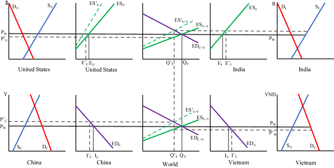
Figure 1. Four-country trade model.
The domestic markets for the United States, India, China, and Vietnam are characterized in the upper left, upper right, bottom left, and bottom right graphs, respectively. The domestic markets in the United States and India present autarky equilibria (the intersection of domestic supply and demand curves) that are below the free trade world price,  ${P_W},$ which indicates that the United States and India are exporting countries. The US excess supply curve, $E{S_U},$ is the difference between its domestic supply and demand curves and is drawn in the adjacent graph. Similarly, Indian excess supply, $E{S_I},$ is drawn next to its domestic market. The sum of these two excess supply curves is the total excess supply, $E{S_{U + I}},$ which appears in the upper middle graph and is also translated into the bottom middle graph. These middle graphs represent the world market and are identical to each other. The reason for including a world market graph in both the upper and bottom sections is to transmit the prices that are determined in the world market equilibrium to each of the four countries’ domestic markets. The autarky equilibria in the Chinese and Vietnamese domestic markets are above the free trade world price, implying that China and Vietnam are importing countries. The Chinese excess demand curve, $E{D_C},$ is the difference between domestic demand and supply, which is drawn in the adjacent graph. Similarly, the Vietnamese excess demand curve, $E{D_V},$ is drawn next to its domestic market. The sum of these two excess demand curves is the total excess demand, $E{D_{C + V}},$ which is also included in the world market graphs. The free trade equilibrium is found at the intersection of the total excess supply and total excess demand curves, which determines the world equilibrium quantity traded, ${Q_T},$ and equilibrium price, ${P_W}.$ The effects of the decline in Yuan value are also depicted in Figure 1 and will be explained along with the comparative static results below.
To obtain comparative static results, we totally differentiate the system of equations in (4)–(7), treating transport costs and tariffs as constants, and place them in matrix form Ax =b (See below equation (4) in the Appendix for these steps):
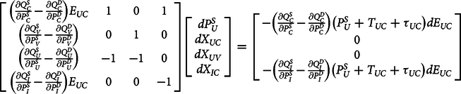 $$\left[{\matrix{ {\left( {\frac{{\partial Q_C^S}}\over{{\partial P_C^S}}} - {\frac{{\partial Q_C^D}}\over{{\partial P_C^D}}} \right){E_{UC}}} 1 0 1\cr\\{\left( {\frac{{\partial Q_V^S}}\over{{\partial P_V^S}}} - {\frac{{\partial Q_V^D}}\over{{\partial P_V^D}}} \right)} {0} {1} {0}\cr \\{\left( {\frac{{\partial Q_U^S}}\over{{\partial P_U^S}}} - {\frac{{\partial Q_U^D}}\over{{\partial P_U^D}}} \right)} { - 1} { - 1} 0\cr\\{\left( {\frac{{\partial Q_I^S}}\over{{\partial P_I^S}}} - {\frac{{\partial Q_I^D}}\over{{\partial P_I^D}}} \right){E_{UC}}} 0 0 { - 1}}}\right]\left[{\matrix{{{dP_U^S}}\cr \\{d{X_{UC}}}\cr\\{d{X_{UV}}}\cr\\{d{X_{IC}}}}} \right] = \left[{\matrix{{- \left( {\frac{{\partial Q_C^S}}\over{{\partial P_C^S}}} - {\frac{{\partial Q_C^D}}\over{{\partial P_C^D}}} \right)\left( P_U^S + {T_{UC}} + {\tau _{UC}} \right)d{E_{UC}}}\cr {0} \cr 0 \cr\\{ - \left( {\frac{{\partial Q_I^S}}\over{{\partial P_I^S}}} - {\frac{{\partial Q_I^D}}\over{{\partial P_I^D}}} \right)\left( {P_U^S + {T_{UC}} + {\tau _{UC}}} \right)d{E_{UC}}}}}\right]$$
The above system is solved using Cramer’s rule to determine the comparative static effects of a change in the exchange rate,  ${E_{UC}},$ on the endogenous variables. The determinant of the coefficient matrix A is
 $$\left| {\bi A} \right| = - \left[ {\left( {\frac{{\partial Q_U^S}}\over{{\partial P_U^S}}} - {\frac{{\partial Q_U^D}}\over{{\partial P_U^D}}} \right) + \left( {\frac{{\partial Q_I^S}}\over{{\partial P_I^S}}} - {\frac{{\partial Q_I^D}}\over{{\partial P_I^D}}} \right){E_{UC}} + \left( {\frac{{\partial Q_C^S}}\over{{\partial P_C^S}}} - {\frac{{\partial Q_C^D}}\over{{\partial P_C^D}}} \right){E_{UC}} + \left( {\frac{{\partial Q_V^S}}\over{{\partial P_V^S}}} - {\frac{{\partial Q_V^D}}\over{{\partial P_V^D}}} \right)} \right] \lt 0.$$
 The negative sign of the determinant of the coefficient matrix is important in ascertaining the direction of the analytical results. Specifically, the sign of the numerator in the following comparative static analysis is reversed by the negative sign of  $\left| {\bi A} \right|$ in the denominator. The magnitude of this determinant hinges upon the supply and demand slopes of each country included in the model. This is because the world price is determined by the interactions of excess supply and excess demand of all countries. Thus, the effects of the decline in Yuan value on the world price reverberates through these slopes (elasticities).
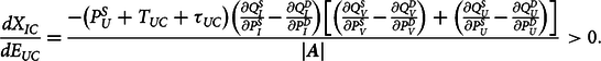
The effect of a fall in Yuan value on US cotton exports to China is
 $${\frac{{d{X_{UC}}}}\over{{d{E_{UC}}}}} = {\frac{{\left( {P_U^S + {T_{UC}} + {\tau _{UC}}} \right)\left[ {\left( {\frac{{\partial Q_I^S}}\over{{\partial P_I^S}}} - {\frac{{\partial Q_I^D}}\over{{\partial P_I^D}}} \right) + \left( {\frac{{\partial Q_C^S}}\over{{\partial P_C^S}}} - {\frac{{\partial Q_C^D}}\over{{\partial P_C^D}}} \right)} \right]\left[ {\left( {\frac{{\partial Q_V^S}}\over{{\partial P_V^S}}} - {\frac{{\partial Q_V^D}}\over{{\partial P_V^D}}} \right) + \left( {\frac{{\partial Q_U^S}}\over{{\partial P_U^S}}} -{ \frac{{\partial Q_U^D}}\over{{\partial P_U^D}}} \right)} \right]}}\over{{\left| {\bi A} \right|}}}}}} \lt 0.$$
 In response to a decrease in Yuan value, US cotton exports to China decline because US cotton, relative to other exporters’ cotton, is more expensive in the Chinese market. The qualitative change in US cotton exports is graphically illustrated in Figure 1, where the drop in Yuan value causes a leftward rotation of the US excess supply curve from  $E{S_U}$ to $E{S'_U}.$Footnote 9 This is because the value of the Yuan in terms of US dollar is lower and, consequently, the United States will expect to receive more Yuan per unit of exports or, in other words, the United States will export less at any given price, which is reflected by the US excess supply curve rotating upward. This causes the total excess supply curve to rotate, $E{S_{U + I}}$ to $E{S'_{U + I}},$ and the world equilibrium after the fall in Yuan value is at the intersection of the new total excess supply curve, $E{S'_{U + I}},$ and initial total excess demand curve, $E{D_{C + V}}$. Therefore, the equilibrium quantity traded decreases from ${Q_T}$ to ${Q'_T},$ and US exports decline from ${E_U}$ to ${E'_U}$.Footnote 10
The impact of a decline in Yuan value on US producer price is
 $${\frac{{dP_U^S}}\over{{d{E_{UC}}}}} = {\left( {P_U^S + {T_{UC}} + {\tau _{UC}}} \right){\frac{{\left( {\frac{{\partial Q_I^S}}\over{{\partial P_I^S}}} - {\frac{{\partial Q_I^D}}\over{{\partial P_I^D}}} \right) + \left( {\frac{{\partial Q_C^S}}\over{{\partial P_C^S}}} - {\frac{{\partial Q_C^D}}\over{{\partial P_C^D}}} \right)}}\over{{\left| {\bi A} \right|}}} \lt 0.}$$
 A fall in Yuan value decreases US exports to China and more is sold within the US market, leading to a lower price. This decline in the US price is illustrated in Figure 1, where the US price decreases from  ${P_W}$ to ${P'_U}.$ At this new lower US price, domestic cotton supply falls, harming US cotton producers. In contrast, the Chinese price, traced from the intersection of $E{S'_{U + I}}$ and $E{D_{C + V}},$ increases from ${P_W}$ to ${P'_C},$ as less US cotton is imported by China. In response to this higher price, Chinese producers increase their cotton production, and Chinese cotton users decrease their demand. From this graphical analysis, we can observe the price wedge, that is, higher Chinese price and lower US price, caused by the exchange rate change.
The comparative static result of a decline in Yuan value on US exports to Vietnam is
 $${\frac{{d{X_{UV}}}}\over{{d{E_{UC}}}}} = {\frac{{ - \left( {P_U^S + {T_{UC}} + {\tau _{UC}}} \right)\left( {\frac{{\partial Q_V^S}}\over{{\partial P_V^S}}} - {\frac{{\partial Q_V^D}}\over{{\partial P_V^D}}} \right)\left[ {\left( {\frac{{\partial Q_I^S}}\over{{\partial P_I^S}}} - {\frac{{\partial Q_I^D}}\over{{\partial P_I^D}}} \right) + \left( {\frac{{\partial Q_C^S}}\over{{\partial P_C^S}}} - {\frac{{\partial Q_C^D}}\over{{\partial P_C^D}}} \right)} \right]}}\over{{\left| {\bi A} \right|}}} \gt 0.$$
 As a result of the decline in value of the Yuan, the United States augments its exports to Vietnam because US exporters are seeking to expand their sales to other importers in order to mitigate lost sales to China. Furthermore, the lower US price incentivizes Vietnamese cotton users to import more from the United States. These changes are shown graphically in Figure 1 where the price in Vietnam falls from  ${P_W}$ to ${P'_W},$ and Vietnam’s imports increase from ${I_V}$ to ${I'_V}.$
The effect of a fall in Yuan value on Chinese imports from India is
 $${\frac{{d{X_{IC}}}}\over{{d{E_{UC}}}}} = {\frac{{ - \left( {P_U^S + {T_{UC}} + {\tau _{UC}}} \right)\left( {\frac{{\partial Q_I^S}}\over{{\partial P_I^S}}} - {\frac{{\partial Q_I^D}}\over{{\partial P_I^D}}} \right)\left[ {\left( {\frac{{\partial Q_V^S}}\over{{\partial P_V^S}}} - {\frac{{\partial Q_V^D}}\over{{\partial P_V^D}}} \right) + \left( {\frac{{\partial Q_U^S}}\over{{\partial P_U^S}}} - {\frac{{\partial Q_U^D}}\over{{\partial P_U^D}}} \right)} \right]}}\over{{\left| {\bi A} \right|}}} \gt 0.$$
 This result shows that Yuan decline relative to the US dollar causes China to increase its imports from other exporters, such as India. Since US cotton exports to China decrease, the Chinese importers fill some of the void with imports from other exporters and also purchases from domestic producers. These changes are depicted in Figure 1 with the increase in Indian exports from  ${E_I}$ to ${E'_I}.$ Because of the higher price in China, overall demand is lower and Chinese imports fall from ${I_C}$ to ${I'_C}.$
Note that the determinant of the coefficient matrix A appears in the denominator of each of the comparative static results. Therefore, the magnitude of each result is dependent on the supply and demand slopes, that is, elasticities, of all countries. The SEM captures the bilateral trade flow changes between any pair of countries which depend on these elasticities. That is why the SEM is highly suitable for analyzing exchange rate changes.
Empirical Model
The four-country theoretical (graphical) model concisely conveys the quantitative (qualitative) impacts of a fall in Yuan value on a pair of exporters and a pair of importers. The comparative statics show the basic trade reallocations that take place as a result of the Yuan–Dollar exchange rate change. These results reflect the expected trade diversions in a world market with only two exporters and two importers; however, the real-world cotton market consists of numerous exporters and importers allowing for many trade reallocations to take place. Consequently, we include 58 regions in the empirical model. The basis of the SEM, from which the market-clearing and spatial-arbitrage conditions of the theoretical model are derived, is an optimization problem. To begin setting up this optimization problem, first consider the following linear supply and demand functions:
 $$p_i^D = {a_i} - {b_i}q_i^D,{\kern 1pt} i = 1,...,N$$
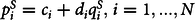 $$p_i^S = {c_i} + {d_i}q_i^S,{\kern 1pt} i = 1,...,N$$
where  $p_i^D$ is the regional demand price, ${a_i}$ is the demand intercept, ${b_i}$ is the demand slope, $q_i^D$ is the demand quantity, $p_i^S$ is the regional supply price, ${c_i}$ is the supply intercept, ${d_i}$ is the supply slope, and $q_i^S$ is the supply quantity in country $i.$ We utilize these inverse supply and demand functions to set up the SEM optimization problem:
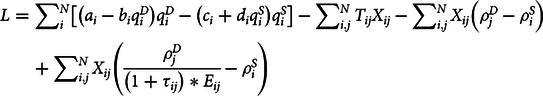 $${L = \sum\nolimits_i^N \left[ {\left( {{a_i} - {b_i}q_i^D} \right)q_i^D - \left( {{c_i} + {d_i}q_i^S} \right)q_i^S} \right] - \sum\nolimits_{i,j}^N {T_{ij}}{X_{ij}} - \sum\nolimits_{i,j}^N {X_{ij}}\left( {\rho _j^D - \rho _i^S} \right) + \sum\nolimits_{i,j}^N {X_{ij}}\left( {\frac{{\rho _j^D}}\over{{\left( {1 + {\tau _{ij}}} \right)*{E_{ij}}}}} - {\rho _i^S} \right)}$$
subject to
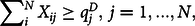 $$\sum\nolimits_i^N {X_{ij}} \ge q_j^D,{\kern 1pt} {\kern 1pt} j = 1,...,N,$$
 $$q_i^S \ge \sum\nolimits_j^N {X_{ij}},{\kern 1pt} {\kern 1pt} i = 1,...,N,$$
 $$\rho _i^D \ge {a_i} - {b_i}q_i^D,{\kern 1pt} {\kern 1pt} i = 1,...,N,$$
 $${c_i} + {d_i}q_i^S \ge \rho _i^S,{\kern 1pt} {\kern 1pt} i = 1,...,N,$$
 $$\left( {\rho _i^S - {S_i} + {T_{ij}}} \right)\left( {1 + {\tau _{ij}}} \right)*{E_{ij}} \ge \rho _j^D,{\kern 1pt} {\kern 1pt} i,j = 1,...,N,$$
and
 $$q_i^D,{\kern 1pt} q_i^S,{\kern 1pt} \rho _i^D,{\kern 1pt} \rho _i^S,{\kern 1pt} {X_{ij}} \ge 0,{\kern 1pt} {\kern 1pt} i,j = 1,...,N,$$
where  ${T_{ij}}$ is the per-unit transport cost from $i$ to $j,$
$j,$ ${X_{ij}}$ is the quantity traded from $i$ to $j,$
$j,$ $\rho _j^D$ is the market demand price in $j,$
$j,$ $\rho _i^S$ is the market supply price in $i,$
$i,$ ${\tau _{ij}}$ is the ad valorem tariff imposed on $i$ by $j,$
$j,$ ${S_i}$ is the domestic subsidy in $i,$ and ${E_{ij}}$ is the exchange rate between $i$ and $j.$
$j.$
The Lagrangian above maximizes the net social monetary gain function of the world cotton market. The interpretation of each term in the Lagrangian is as follows. The SEM maximizes the sum of all countries’ sales revenues,  $\sum\nolimits_i^N \left( {{a_i} - {b_i}q_i^D} \right)q_i^D,$ minus producers’ revenues, $\sum\nolimits_i^N \left( {{c_i} + {d_i}q_i^S} \right)q_i^S,$ minus transport costs, $\sum\nolimits_{i,j}^N {T_{ij}}{X_{ij}},$ minus the loss resulting from the price wedge created by a change in the currency value, $ {- \left[ {\sum\nolimits_{i,j}^N {X_{ij}}\left( {\rho _j^D - \rho _i^S} \right)} - {\sum\nolimits_{i,j}^N {X_{ij}}\left( {\frac{{\rho _j^D}}\over{{\left( {1 + {\tau _{ij}}} \right)*{E_{ij}}}}} - {\rho _i^S} \right)} \right].}$ Constraints a) and b) are the market-clearing constraints, similar to those of the theoretical model. The first ensures that the total quantity imported by $j,$ including from itself, is greater than or equal to the total demand in $j.$ The second states that the total quantity exported by $i,$ including to itself is less than or equal to the total supply in $i.$ Constraint c) requires that the market demand price is greater than or equal to the regional demand price. Constraint d) entails the regional supply price is greater than or equal to the market supply price. Note, the market demand (supply) price will be exactly equal to the regional demand (supply) price when there is an interior solution, but greater (less) than the regional demand (supply) price when there is a corner solution. Constraint e) restricts the market demand price in the importing region to be less than or equal to the market supply price minus the domestic subsidy plus transport, tariff, and exchange rate costs. Lastly, constraint f) states that all endogenous variables are nonnegative.
The above maximization problem yields first-order conditions consisting of  $3,596$ equations ( $58$ demand constraints, $58$ supply constraints, $58$ market versus regional demand price constraints, $58$ market versus regional supply price constraints, and $58 \times 58$ price linkage equations) and $3,596$ endogenous variables ( $58$ demand quantities, $58$ supply quantities, $58$ market demand prices, $58$ market supply prices, and $58 \times 58$ bilateral trade flows). This square system of equations is solved simultaneously, and any trade reallocations among countries in response to a change in currency value are determined.
Data and Empirical Analysis
The  $58$ regions in the empirical model consist of $57$ major cotton producing, consuming, and trading regions plus an aggregate ROW region. These $58$ regions account for all cotton production, consumption, and trade in the world. Solving the empirical model requires the construction of supply and demand functions, and values for exogenous variables ( $T,{\kern 1pt} {\kern 1pt} \tau ,$ and $E$). To construct the supply and demand functions, we compute the intercept and slope parameters using production, consumption, price, and elasticity data for each region. Production, consumption, and price data were gathered from U.S. Department of Agriculture (2018, 2019) and are average values over a 3-year period prior to the trade dispute (2015 to 2017). The production and consumption values for the ROW region are calculated by subtracting the total production and consumption of the 57 regions from the total world production and consumption values. For ROW price, we use the world price in 2017, which was obtained from Statista (2019).
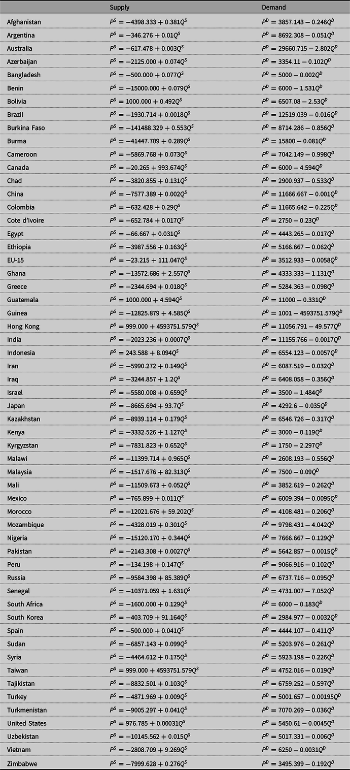
Demand elasticities were obtained from Poonyth et al. (Reference Poonyth, Sarris, Sharma and Shui2004) for 28 of the countries included. Of these 28 countries, 23 of them have demand elasticities of −0.60. The elasticities of the remaining five countries are: China and Pakistan −1.00, Columbia and Mexico −1.30, and India −0.8. For the remaining 29 countries, we considered demand elasticities of −0.6, consistent with the estimates for most of the countries in Poonyth et al. (Reference Poonyth, Sarris, Sharma and Shui2004). Thus, the demand elasticities range in absolute values from a low of −0.6 to a high of −1.3, with a mean elasticity of −0.642. The supply elasticities for 28 countries (reported in Poonyth et al. (Reference Poonyth, Sarris, Sharma and Shui2004)) are the average between the supply elasticities found in Poonyth et al. (Reference Poonyth, Sarris, Sharma and Shui2004) and Shepherd (Reference Shepherd2006). Shepherd (Reference Shepherd2006) has elasticities for eight additional countries that were not covered by Poonyth et al. (Reference Poonyth, Sarris, Sharma and Shui2004), and we used the supply elasticities for these eight countries from Shepherd. For the remaining 21 countries, we utilized supply elasticities of 0.8, which is the supply elasticity for the majority of the 28 countries in Poonyth et al. (Reference Poonyth, Sarris, Sharma and Shui2004). Countries with small supply elasticities are Nigeria (0.251), Cote d’Ivoire (0.339), and Cameroon (0.386), and countries with large supply elasticities are Argentina (1.044), and Bangladesh and Turkmenistan (1.2). The supply elasticities range from a low of 0.251 to a high of 1.2, with a mean elasticity of 0.719. Using the elasticity formula,  ${\varepsilon _i} = {\frac{dq_i^S}\over{dp_i^S}}{\frac{p_i^S}\over{q_i^S}}$, and the obtained price and production values, the supply slope is calculated as
 $${\frac{{dq_i^S}}\over{{dp_i^S}}} = {\varepsilon _i}{\frac{{q_i^S}}\over{{p_i^S}}} = {D_i}.$$
Using this slope parameter, the supply intercept is computed as
 $${C_i} = q_i^S - {D_i}p_i^S.$$
The resulting supply function is  $q_i^S = {C_i} + {D_i}p_i^S$, which is then converted into inverse supply equation (13) with intercept ${c_i}$ and slope ${d_i}.$ We construct the inverse demand equation in a similar fashion.
With the computed inverse demand and supply functions, we can run the baseline. However, the baseline solutions for the endogenous variables may not replicate the actual data for these variables because the constructed demand and supply functions are based on elasticities which came from several studies. These studies used different periods and functional forms to estimate these elasticities. To match the baseline solutions to actual data, we calibrate the model by matching the solved values of production, consumption, and trade flows to actual data. For this calibration, we employ the calibration procedure developed by Paris et al. (Reference Paris, Drogué and Anania2009), which adjusts the supply and demand parameters and transport costs such that the model’s baseline results replicate the actual values of the endogenous variables.Footnote 11 The data sources for these variables are given above, with the exception of bilateral trade flow data, which came from Simoes and Hidalgo (Reference Simoes and Hidalgo2019). Tariff data for each region were found at World Trade Organization (2019) and Government of Canada (2017). The ROW region, being a conglomerate of several regions, does not have bilateral tariff data of its own. However, any tariffs imposed by or on the ROW region are accounted for in the transportation cost via the calibration process. Furthermore, subsidy data was taken from Hudson (Reference Hudson2018) and EWG (2019), and the Yuan–Dollar exchange rate was collected from International Monetary Fund (2019). Transport costs were obtained using the World Freight Rates (2019) online freight calculator for an average cotton price of $1816.95/metric ton with a 10,000 metric ton (MT) break bulk load. For regions with multiple ports, calculations were made based on the shortest port-to-port distance. For landlocked countries, we included additional transportation costs based on the distance from the nearest port at a price of 0.09$/ton/mile (Qiao and Paggi, Reference Qiao and Paggi2019).
After the model is calibrated, we run two scenarios: a baseline and an alternate. The baseline maintains the Yuan–Dollar exchange rate before the US–China trade war. In the alternate scenario, we increase the Yuan–Dollar exchange rate by 12.6% which implies the Yuan fell relative to the US dollar by 12.6%. The results of the alternate scenario are compared to the baseline scenario to determine the effects of this decline in Yuan value on endogenous variables.
Results
Table 1 reports the baseline results for production, consumption, supply price, and demand price for the leading  $25$ regions along with the impacts (in percent changes) of the fall in Yuan value.Footnote 12 Table 2 presents the effects of the decline in the value of the Yuan on producer and consumer surplus, tariff revenues, and net welfare changes. The empirical analysis generates $3,364$ ${(58 \times 58)}$ values for bilateral trade flows, and it is not plausible to present all of these results. Consequently, we report key trade flow results of major importers of US cotton in Table 3 and major exporters of cotton to China in Table 4.
Table 1. Baseline scenario results and impacts of the Yuan–Dollar exchange rate change

Table 2. Effects of the Yuan–Dollar exchange rate change on surplus measures
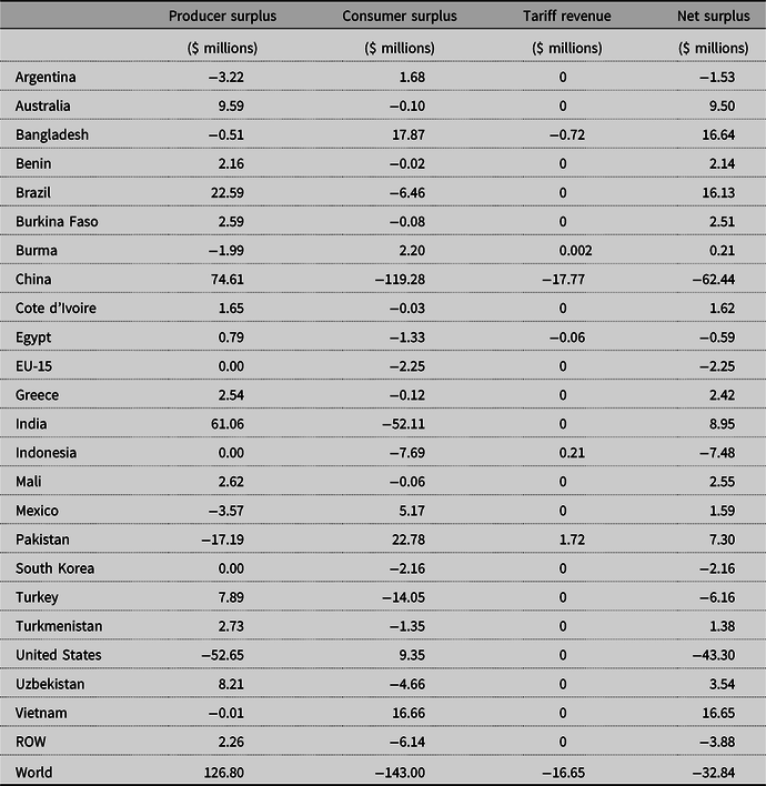
Table 3. US exports (1000 MT)

Table 4. Chinese Imports (1000 MT)
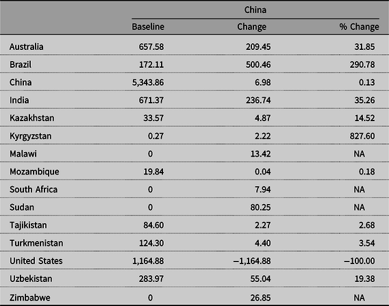
Table 1 shows that the fall in Yuan value has both positive and negative effects on the world cotton market. Many countries experience a decrease in price, harming producers and benefiting consumers, while other countries see an increase in price, benefiting producers but hurting consumers. These changes are expected from an economic shock such as a change in currency value. Specifically, this policy is harmful to US cotton producers because the 12.6% decline in Yuan value causes US cotton exports to China to be completely eliminated as US cotton becomes relatively more expensive for Chinese cotton users. This causes US producers to sell more in the domestic market, which drives down the US supply price by 0.63%. This price reduction causes US producers to decrease production by 1.04%. The US demand price falls by 0.71%, leading to an increase in domestic use by 0.41%.Footnote 13 To mitigate the export loss to China, the United States seeks to export elsewhere. As a result, the United States expands its exports to nine other importing countries, which greatly lessens the adverse effects of the lower value in Yuan on price, production, and consumption. Specifically, the United States augments its exports to other major textile producers such as Bangladesh, Mexico, and Vietnam, as reported in Table 3. Because of these reallocations, the decrease in US price and production are relatively small. The United States has the ability to reallocate its exports because cotton is a heavily used and highly traded commodity in the world market. Stated differently, if the United States did not have abundant reallocation opportunities, the adverse effects of the change in Yuan–Dollar exchange rate would be more severe. In spite of the small percentage declines in price and production, the US producer surplus loss is $52.65 million because of the voluminous cotton production (Table 2). Though US cotton users enjoy a $9.35 million increase in consumer surplus as a result of the domestic price decrease, the overall effect of the drop in Yuan value is negative with a $43.30 million loss in net surplus.
The decline in the Yuan value has largely different effects in China than it does in the United States, but the net outcome is also a loss. Chinese consumers decrease imports of US cotton as it becomes more expensive and augment imports from other exporters such as Brazil, India, and a host of smaller exporters (Table 4). Some of these exporters had not previously, that is, before the exchange rate change, exported cotton to China. Though cotton imports from other exporters increase, it is not enough to offset the lost imports from the United States, which, as stated above, are fully expunged. As a result, there is a shortage of cotton in China, which causes the Chinese demand price to increase by 0.51% and overall consumption to decrease by 0.16%. Chinese supply price increases by 0.46%, causing producers to expand production by 0.13%. Table 0 shows that China incurs a $119.28 million loss in consumer surplus and a $74.61 million gain in producer surplus. As imports of US cotton are completely expunged and replaced with imports, albeit less, from other exporters, Chinese tariff revenue falls by $17.77 million. The combined effect of these surplus measure changes is a $62.44 million loss in net surplus.
Brazil, India, and Australia are the three leading cotton exporters following the United States. Brazil increases its exports to China by 500,460 metric tons (290.78%), which crowds out cotton supply domestically and causes a price increase of 0.57%. This rise in price expands Brazilian production by 0.24% and lowers consumption by 0.10%. As a result of these changes, Brazil’s producer surplus increases by $22.59 million, consumer surplus decreases by $6.46 million, and net surplus rises by $16.13 million. This gain in net surplus is the largest among exporters. The effects of the fall in Yuan value on the Indian and Australian markets are comparable to those of Brazil. Indian exports to China increase by 236,740 metric tons (35.26%), which causes the Indian price to rise by 0.54%, production to increase by 0.23%, and consumption to fall by 0.11%. Similarly, Australian exports to China increase by 209,450 metric tons (31.85%), causing Australia’s price to rise by 0.53%, production to increase by 0.35%, and consumption to fall by 0.04%. These changes lead to a $61.06 ($9.59) million increase in producer surplus, $52.11 ($0.10) million decrease in consumer surplus, and $8.95 ($9.50) million rise in net surplus for India (Australia).
Several exporting countries–Afghanistan, Argentina, Israel, and Syria–do not increase cotton exports to China and in fact decrease their overall exports in response to changes in Yuan value. This is because the prices in these countries are not competitive relative to exporters such as Brazil and India. Additionally, these countries lose exports to importing countries that are now importing from the United States at a reduced price. For example, Argentinian exports to Mexico decrease by 32,897 metric tons (not reported), as Mexico increases its imports from the United States by 35,460 metric tons. This causes a relative surplus of cotton supply in the Argentinian domestic market, which causes its price to decline by 0.76%, production to fall by 0.53%, and consumption to increase by 0.20%. As a result, Argentinian producer surplus shrinks by $3.22 million, consumer surplus rises $1.68 million, and overall welfare declines $1.53 million. These adverse effects on Argentina are caused by the web of trade reallocations that take place in response to the change in Yuan value, which are aptly captured by the SEM. This is the primary reason for using the SEM for this analysis.
Besides China, the three largest importers of cotton are Bangladesh, Vietnam, and Indonesia. Bangladesh increases its imports from the United States by 544,590 metric tons, which causes the price in Bangladesh to fall 0.69%. This decrease in price leads to a fall in production of 0.47% and a rise in consumption of 0.53%. Consequently, producer surplus in Bangladesh decreases $0.51 million, while consumer surplus increases by $17.87 million. Additionally, tariff revenue in Bangladesh falls $0.72 million due to its reallocation of higher priced imports to lower priced imports from the United States. Because the Bangladesh tariff is an ad valorem tariff, it is a percentage of the import price and, consequently, by importing cotton at the lower US price the overall tariff revenue falls. The combined surplus measure changes lead to an overall increase of $16.64 million in Bangladesh’s welfare. Vietnam experiences a 4,760 metric ton increase in imports from the United States which causes the domestic price to fall by 0.69%, production to decline by 0.22%, and consumption to rise 0.33%. These changes lead to a decrease in producer surplus of $0.01 million, an increase in consumer surplus of $16.66 million, and net welfare rises by $16.65 million. Indonesia, unlike Bangladesh and Vietnam, does not increase its imports from the United States and, in fact, loses 1,837 metric tons worth of imports from Brazil (not reported) as Brazil diverts its exports to China. Therefore, a relative shortage of cotton supply in Indonesia compared to that in the baseline scenario occurs, which leads to a price increase of 0.53%. This causes an increase in domestic production of 0.49% and a decrease in consumption of 0.25%. As a result, Indonesia’s producer surplus increases $0.003 million and its consumer surplus decreases by $7.69 million. However, even though Indonesia’s total import volume decreases, its tariff revenue increases by $0.21 million. This is because Indonesia’s tariff is an ad valorem tariff and, consequently, as the prices rise in the countries that Indonesia imports from (Brazil, India, etc.), the tariff revenue collected by Indonesia rises. Ultimately, Indonesian net welfare decreases by $7.48 million as a result of the lower value in Yuan.
The majority of the remaining importing countries benefit from the change in Yuan value as they increase their imports from the United States or from other exporting countries that are seeking to find additional export markets after the United States replaced some of their previous sales. Some importers (e.g., Egypt, Ethiopia, EU-15, Hong Kong, Iran, Iraq, Japan, Kenya, Morocco, Russia, South Korea, Taiwan, and Turkey), similar to Indonesia, are harmed, but these importers do not see the increase in tariff revenue that Indonesia does, and are therefore unable to mitigate their net welfare losses. The impacts of the decline in the value of the Yuan on total world surplus measures are an increase in the world producer surplus of $126.80 million, a loss in consumer surplus of $143.00 million, a loss in tariff revenue of $16.65 million, and an overall world net welfare loss of $32.84 million.
A sensitivity analysis on the elasticities of the three major exporters (Brazil, India, and the United States) was conducted to test the robustness of the model. Rather than changing the elasticities for all countries, we recalculated the supply equations for Brazil, India, and the United States once with elasticities increased by 50% and once decreased by 50%. We then ran the SEM with the new supply equations for Brazil, India, and the United States and compared the results with those of the original. We found that both the increase and decrease in elasticities made only slight changes in the results. For instance, in the original model, the changes in supply caused by the fall in Yuan value for Brazil, India, and the United States were 0.245%, 0.233%, and −1.038%, respectively. In the model with decreased elasticities, the respective changes were 0.111%, 0.104%, and −0.562%, respectively. Lastly, in the model with increased elasticities, the changes in supply for Brazil, India, and the United States were 0.106%, 0.099%, and −0.443%, respectively.Footnote 14 US exports to China are fully expunged in all three models, while the percent change in US exports to other importers are nearly identical between models, that is, US exports to Canada increase by 0.349% in the original model, 0.387% in the decreased elasticity model, and 0.101% in the increased elasticity model. The trade flow changes for Brazil and India are very close for each of the three models.
Conclusions
The trade dispute between the United States and China has worsened with each country imposing escalating tariffs on a vast number of commodities, which has distorted the world trade order. The loss in China from this trade war is mitigated by the decline in the Yuan relative to the US dollar. In the wake of this trade dispute, many studies have examined the effects of both countries’ tariffs on various commodity markets. However, to our knowledge, no study has analyzed the effects of the change in Yuan–Dollar exchange rate. Because of the decline in Yuan value relative to the US dollar, Chinese goods have become less expensive for US consumers which counteracts the effects of US tariffs imposed on Chinese goods. Additionally, because the value of the US dollar is higher relative to the Yuan, US goods have become more expensive for Chinese consumers which reinforces the effects of the Chinese tariffs imposed on US goods. This paper analyzes the effects of the decline in Yuan value, in isolation of tariffs, on US, Chinese, and world cotton markets. Cotton was chosen for analysis because a) of its importance in the world market as numerous countries produce, consume, and trade cotton, b) it is a major commodity in the United States and China, c) the United States is the largest exporter, and d) China is the second largest importer.
This study utilizes the SEM to conduct the analysis of the effects of Yuan–Dollar exchange rate changes on world cotton markets. The SEM aptly captures the trade reallocations that occur as a result of economic shocks such as changes in currency values. The theoretical model outlines the basis of the SEM using a four-country model and finds the comparative static results for the effects of changes in the Yuan–Dollar exchange rate on prices and trade flows. This model is then implemented empirically for  $58$ regions to determine quantitative results of the effects of this change.
The results show that a decline in the Yuan value has negative effects on many countries that participate in world cotton trade. The United States and China incur the largest losses as a result of the Yuan–Dollar exchange rate change, with the United States losing $43.30 million in net welfare and China losing $62.44 million. Some exporting countries benefit greatly at the expense of the United States, particularly Brazil and India. These two countries expand their exports to China, respectively, by 500,460 metric tons and 236,740 metric tons and augment their net welfare by $16.13 million and $8.95 million. However, other exporters, such as Argentina, are harmed by the the lower Yuan. Argentina’s total exports decline as the United States captures some of its export market. This leads to a $1.53 million fall in Argentina’s net welfare. Many importing countries see a rise in welfare as the United States reallocates its exports from China to these countries and sells at its new lower price. Bangladesh and Vietnam gain the most as these two countries’ welfare increase by $16.64 million and $16.65 million, respectively. But, some importers incur net welfare losses as new imports from the United States are less than the lost imports from other exporters who reallocated their sales to China. The world as a whole incurs a $32.84 million loss in welfare as a consequence of the drop in Yuan value.
These results highlight the adverse effects of the change in currency values and reinforce the theory that restrictive trade policies through exchange rate changes are overall welfare reducing. The fall in Yuan value lessens the effects of US tariffs on Chinese imports and reinforces the effects of their own tariffs, but creates a loss to China overall. The findings of this study are useful for cotton producers, agribusiness firms, textile users, exporters, importers, and policy makers. Given the adverse impacts of Chinese policies on the US cotton market, US producers may want to mitigate the negative consequences by exporting to other cotton using countries. For example, US producers can target Bangladesh and Vietnam because these countries increase cotton imports in response to the Yuan–Dollar exchange rate changes. However, the long-term solution is to move toward free trade and avoid unwanted stress on US commodity producers. It is important to note that the model used in this study isolates the effects of the Yuan–Dollar exchange rate change and therefore does not consider other trade policies that exist between countries. Consequently, though the results are useful for policy makers, cotton producers should be aware that there are additional policies affecting the price and trade of cotton that are not modeled here. In addition, this model is a partial equilibrium model and does not take into account the impacts on upstream or downstream sectors. In particular, the impacts on textile industries in the downstream sector are not studied.
Acknowledgment
The authors thank the editor Sayed Saghaian for effective review coordination and anonymous reviewers for providing useful suggestions. This work was supported by the USDA National Institute of Food and Agriculture, Agricultural and Food Research Initiative Competitive Program, Agriculture Economics and Rural Communities, grant # 2019-12907613.
Supplementary material
To view supplementary material for this article, please visit https://doi.org/10.1017/aae.2020.12
Appendix
Appendix Table A1: Supply and demand equations


 Open access