


1. Introduction
1.1. Radar layers
Ice-penetrating radars (IPR) were developed to measure ice thickness in polar ice sheets (Reference Paren and RobinParen and Robin, 1975). These radars can also detect internal layers, which are commonly interpreted as horizons of constant age (isochrones). These layers can be used to infer the history of ice sheets, including migration of ice divides (Reference Nereson, Raymond and JacobelNereson and others, 1998), changes in thickness, and initiation of new ice divides (e.g. Reference Conway, Hall and DentonConway and others, 1999; Reference Nereson and RaymondNereson and Raymond, 2001). The depths of these layers also provide information on accumulation-rate patterns; however, the most appropriate technique to extract this information depends on the amount of strain that the ice has experienced.
1.2. Strain regimes
In the uppermost few percent of an ice sheet, ground-penetrating radars (GPR) also detect layers, and local accumulation rate can be viewed as directly proportional to ice-equivalent layer depth (e.g. Reference Pinglot, Hagen, Melvold and EikenPinglot and others, 2001; Reference Spikes, Hamilton, Arcone and KaspariSpikes and others, 2004). We call this the shallow-layer approximation (SLA).
Since older layers reflect longer-term patterns of climate, there is also strong motivation to extract accumulation patterns from these older layers. As the depth of an internal layer increases to a larger fraction of the total ice thickness, the ice above that layer has been subjected to increasing total strain as a result of ice flow. The SLA is no longer appropriate for layers buried by more than a few percent of the ice thickness. For these layers, a layer-thinning correction must be applied. Accumulation rates have been extracted from these layers by integrating local vertical strain rates in a onedimensional (1-D) flow model to get a strain correction (e.g. Reference Morse and WaddingtonMorse and others, 1999; Reference Vaughan, Corr and DoakeVaughan and others, 1999; Reference Fahnestock, Abdalati and LuoFahnestock and others, 2001; Reference Kanagaratnam, Gogineni and GundestrupKanagaratnam and others, 2001; Reference PälliPälli and others, 2002; Reference Leysinger Vieli, Siegert and PayneLeysinger Vieli and others, 2004; Reference Siegert and PayneSiegert and Payne, 2004). We call this the local-layer approximation (LLA). Using the LLA is equivalent to assuming that there are no horizontal gradients in geometry and strain rate, or that a sandwich model as described by Reference ReehReeh (1989) adequately represents the flow.
However, even the LLA becomes inadequate for deeper layers, where horizontal gradients in accumulation rate and strain rate along particle paths have significantly affected layer depths. Extraction of accumulation-rate information from these layers is a challenging problem that requires a full treatment of ice flow and accumulated strain along particle paths. We define these as deep layers for the purpose of inferring accumulation-rate patterns.
In section 6, we derive non-dimensional numbers that determine whether the SLA, the LLA or a deep-layer treatment should be used for any particular layer. In this paper, we describe a general inverse method to extract accumulation-rate information from deep layers.
1.3. Previous work
Several previous studies have avoided the limitations of the LLA by using flowline particle-tracking models to calculate layer shapes. Reference Nereson, Raymond and WaddingtonNereson and others (2000) used a twodimensional (2-D) flow model to estimate the spatial pattern of accumulation across Siple Dome, Antarctica. They approximated the spatial variation of accumulation rate with an arctangent function, and used an inverse procedure to select the two parameters defining its amplitude and length scale on each side of the divide. Reference Baldwin, Bamber and PayneBaldwin and others (2003) tracked particles backward along trajectories in a steady-state model, starting from two internal layers of known ages in the Greenland ice sheet. They used mismatches between their modelled surface and the observed surface to infer corrections to the measured accumulation pattern. The adjustment algorithm allowed only corrections that varied slowly over length scales greater than the particle-path lengths. Variability over shorter distances could be incorporated only through the initial guess, which was based on previously measured accumulation rates. The algorithm could not create, correct or remove short-wavelength structures. In practice, application of the method was limited to relatively young layers with short particle paths, or to regions with low spatial gradients in accumulation rate, where layer ages are already known. Reference Parrenin and HindmarshParrenin and others (2006) presented analytical solutions for steady-state shapes of deep layers. Reference Hindmarsh, Siegert and GudmundssonHindmarsh and others (2002) used a formal optimal-filter inverse approach to match observed layers, and Reference Martín, Hindmarsh and NavarroMartín and others (2006) used a control-method approach to infer a spatial pattern of accumulation rate from internal layers. Their work bears a strong conceptual connection to the work that we address here, although it used a different inverse approach.
Here, we describe a general, robust procedure using geophysical inverse theory (e.g. Reference MenkeMenke, 1989; Reference ParkerParker, 1994; Reference Aster and BorchersAster and others, 2005) to recover the spatial pattern and magnitude of accumulation rate along a flowband, using a deep layer. The method can recover the information on spatial patterns of accumulation rate as retained in internal-layer geometry, without additional assumptions about scales of variability, or layer age.
1.4. Forward and inverse problems
The forward problem is the calculation of ice-velocity and ice-temperature fields, ice-surface topography and shapes of internal layers. The forward problem is described by a set of conservation and constitutive equations, boundary conditions and parameter values. Those boundary conditions include the spatial pattern of accumulation rate. In the corresponding inverse problem, we know the equations, and we may know some or all of the boundary conditions, and some or all of the parameter values. We incorporate data into the solution procedure in order to infer the remaining unknown boundary conditions and parameters.
In our specific inverse problem, we can use surface-profile and layer-depth information, as well as other data (if available), such as point measurements of surface velocity and accumulation rate, in order to find a smooth accumulation-rate profile and other model parameters that together produce an expected level of mismatch between the data and corresponding values calculated using these model parameters in the forward problem.
Since fully general inverse procedures can be computationally expensive, it is desirable to customize and reduce the complexity of the inverse procedure by exploiting any simplifications that can be justified in each particular application. After describing the inverse procedure in its general form, we apply the method to an internal layer observed along a flowline near Taylor Dome, Victoria Land, Antarctica. By introducing additional approximations that are appropriate to this particular flowline, we illustrate how the general procedure can be simplified for this particular field site.
Notation
We use boldface lower-case type to represent vectors, and single subscripts to indicate their components. We use boldface upper-case type to represent matrices, and double subscripts to denote their components.
2. Forward Problem
We solve our forward problem to find ice-surface elevation, ice velocities and layer shapes, using a flowband with steady-state surface, velocities and temperature. The flowband has variable width W(x), where x follows the flow direction, y is horizontal and transverse to the flow, and z is the vertical coordinate. S(x) is the ice-equivalent surface elevation, ![]() is the bed elevation, (S – z) is the depth below the surface, and H(x) = S(x) –
is the bed elevation, (S – z) is the depth below the surface, and H(x) = S(x) – ![]() is ice-equivalent thickness. Our model can be applied to any limited region of an ice sheet, including those that do not include an ice divide. Our formulation is designed to allow a wide range of thermomechanical calculations to be adapted to it.
is ice-equivalent thickness. Our model can be applied to any limited region of an ice sheet, including those that do not include an ice divide. Our formulation is designed to allow a wide range of thermomechanical calculations to be adapted to it.
2.1. Flowband geometry
With the assumption that flow direction is controlled by the local surface slope, flowlines can be defined as trajectories that are everywhere parallel to the gradient of the measured surface topography. When surface-velocity measurements are also available, that assumption can be relaxed, and flowlines can be defined as trajectories that are everywhere parallel to the measured velocities. A flowband is the volume bounded by two vertical surfaces directly beneath two nearby flowlines. We use a steady-state flowband of variable width W(x), where x follows the ice-flow direction along the center of the flowband, y is horizontal and transverse to the flow, and z is elevation. The bed elevation ![]() must also be known along the flowband. Bed elevation B(x), ice thickness S(x), and the components of velocity v = (u, v, w) in the x and z directions are assumed to be uniform in the y direction transverse to the central flowline. In solving our forward problem, we calculate the steady-state ice-equivalent ice-surface topography S(x), and the steady-state flow field v everywhere in the flowband. The velocity is tangential to the vertical boundaries of the flowband, and u and w are invariant in the y direction across the flowband. Depth below the surface is (S(x) – z), and ice-equivalent thickness is H(x ) = S (x) – B(x).
must also be known along the flowband. Bed elevation B(x), ice thickness S(x), and the components of velocity v = (u, v, w) in the x and z directions are assumed to be uniform in the y direction transverse to the central flowline. In solving our forward problem, we calculate the steady-state ice-equivalent ice-surface topography S(x), and the steady-state flow field v everywhere in the flowband. The velocity is tangential to the vertical boundaries of the flowband, and u and w are invariant in the y direction across the flowband. Depth below the surface is (S(x) – z), and ice-equivalent thickness is H(x ) = S (x) – B(x).
2.2. Rheological parameters
When the coordinates (x, y, z) are written in index notation as (x1, x2, x3), ice strain rate ![]() is calculated from a temperature-dependent flow law (e.g. Reference GlenGlen, 1958; Reference PatersonPaterson, 1994, ch. 5), using
is calculated from a temperature-dependent flow law (e.g. Reference GlenGlen, 1958; Reference PatersonPaterson, 1994, ch. 5), using
where i and j can take values from 1 to 3, τij is the deviatoric stress tensor, τ e is its second invariant, n = 3 is the flow-law exponent, and θ is temperature. A(θ) is a temperature-dependent softness or fluidity parameter; A(θ) is generally written as A o exp(— Q/R θ) (Reference PatersonPaterson, 1994, p. 86), where Q = 60kJ mol∼1 is the activation energy for creep, and R = 8.314J mol∼1 K∼1 is the gas constant. We use A0 = 4.0 x 10∼4 kPa∼3 s∼1, the value derived from Reference PatersonPaterson (1994, p. 97, table 5.2) for temperatures below —10°C. At a given temperature θ, the rheological behavior of ice in our model is fully determined by a single adjustable model parameter, the enhancement factor E. Under other circumstances, E may vary spatially (e.g. to represent a contrast between ice-age and interglacial ice). If ice is treated as an anisotropic material, a different constitutive relation may replace Equation (1), and additional parameters may be introduced.
2.3. Thermomechanical flow calculations
Calculation of surface topography and velocity requires calculation of the temperature field θ, because strain rate ![]() in ice (Equation (1)), basal-sliding rate, and basal-melting rate all depend on the temperature distribution. In many cases, the temperature calculations also depend on ice flow. Any steady-state thermomechanical calculation also requires a specified ice thickness at one location to provide a boundary condition. For example, we might use the measured ice thickness at an ice-core site. When the parameters controlling mass balance, rheological properties and thermal conditions have been specified, the forward problem can be solved using any of a wide variety of ice-flow models to calculate the steady-state surface topography, ice velocity, and temperature. These thermomechanical calculations generally proceed by integrating a rheological relation such as Equation (1), while simultaneously solving a heat-flow equation for the temperature. Because the required complexity of these calculations can be site-specific, we do not describe a general thermomechanical calculation procedure. In Appendix B, we describe a specific simplified thermomechanical calculation procedure that is appropriate for our site at Taylor Mouth, Antarctica.
in ice (Equation (1)), basal-sliding rate, and basal-melting rate all depend on the temperature distribution. In many cases, the temperature calculations also depend on ice flow. Any steady-state thermomechanical calculation also requires a specified ice thickness at one location to provide a boundary condition. For example, we might use the measured ice thickness at an ice-core site. When the parameters controlling mass balance, rheological properties and thermal conditions have been specified, the forward problem can be solved using any of a wide variety of ice-flow models to calculate the steady-state surface topography, ice velocity, and temperature. These thermomechanical calculations generally proceed by integrating a rheological relation such as Equation (1), while simultaneously solving a heat-flow equation for the temperature. Because the required complexity of these calculations can be site-specific, we do not describe a general thermomechanical calculation procedure. In Appendix B, we describe a specific simplified thermomechanical calculation procedure that is appropriate for our site at Taylor Mouth, Antarctica.
2.4. Kinematic representation of velocity
For a given accumulation-rate pattern ![]() and basal melting-rate pattern both expressed in ice-equivalent units, the steady-state ice-flux profile q(x) along the flowband is given by
and basal melting-rate pattern both expressed in ice-equivalent units, the steady-state ice-flux profile q(x) along the flowband is given by
where q in
is the flux entering or leaving the flowband at x = x
in
. At any location x, the flowband has cross-sectional area W(x) x H(x). The ice flux q(x) through the cross-section is also proportional to ![]() the horizontal velocity u(x, z) averaged over that cross-section, through
the horizontal velocity u(x, z) averaged over that cross-section, through
The distribution of velocity with depth depends on the basal boundary conditions and on the selected thermomechanical ice-flow algorithm. In order to make the inverse procedure independent of details of specific algorithms for thermomechanical flow calculations, and to standardize procedures for particle tracking, we represent horizontal velocities u(x, z) along a vertical profile at any position x as the product of the depth-averaged velocity ū(x), and a non-dimensional shape function ![]() (Reference ReehReeh, 1988), which describes how the horizontal velocity varies with depth, giving
(Reference ReehReeh, 1988), which describes how the horizontal velocity varies with depth, giving
where ![]() is normalized non-dimensional height above the bed, given by
is normalized non-dimensional height above the bed, given by
The horizontal-velocity shape function ![]() is produced by the forward algorithm, in which many different thermomechanical ice-flow models can be used. The sophistication required of the thermomechanical model depends on the characteristics of the particular site under investigation. One approach is to use the shape functions
is produced by the forward algorithm, in which many different thermomechanical ice-flow models can be used. The sophistication required of the thermomechanical model depends on the characteristics of the particular site under investigation. One approach is to use the shape functions ![]() generated by a simple kinematic approximation such as the Reference Dansgaard and JohnsenDansgaard and Johnsen (1969) model. A second approach is to use shape functions based on the shallow-ice approximation (SIA; e.g. Reference PatersonPaterson, 1994, p.262), incorporating depth-varying temperature. A third approach, followed by Reference Nereson, Raymond and WaddingtonNereson and others (1998) and by Reference Morse and FeshbachNereson and Waddington (2002), is to use polynomial approximations to the velocity profiles produced by a finite-element momentum-conservation flow model (e.g. Reference RaymondRaymond, 1983; Reference HvidbergHvidberg, 1996) that incorporates all stress components for plane strain, and incorporates the influence of temperature on strain rates.
generated by a simple kinematic approximation such as the Reference Dansgaard and JohnsenDansgaard and Johnsen (1969) model. A second approach is to use shape functions based on the shallow-ice approximation (SIA; e.g. Reference PatersonPaterson, 1994, p.262), incorporating depth-varying temperature. A third approach, followed by Reference Nereson, Raymond and WaddingtonNereson and others (1998) and by Reference Morse and FeshbachNereson and Waddington (2002), is to use polynomial approximations to the velocity profiles produced by a finite-element momentum-conservation flow model (e.g. Reference RaymondRaymond, 1983; Reference HvidbergHvidberg, 1996) that incorporates all stress components for plane strain, and incorporates the influence of temperature on strain rates.
The strain rate transverse to the flowband is (e.g. Reference WaddingtonWaddington, 1982)
The vertical velocity w(x, z) can then be recovered from incompressibility,
At the bed (z = B(x), or ![]() ), the vertical velocity is
), the vertical velocity is
where the first term represents vertical motion due to basal melting, and the second term represents vertical motion due to sliding over basal topography. Melting and sliding can be calculated by appropriate equations or algorithms in the forward problem. A vertical integration of Equation (7) from the bed, together with Equations (2–6) leads to an expression for the vertical velocity:

where
In the absence of basal melting, basal sliding and horizontal gradients in surface elevation, bed elevation and horizontal-velocity shape function, the first term fully describes the vertical velocity; hence, ![]() is sometimes called a vertical-velocity shape function.
is sometimes called a vertical-velocity shape function.
2.5. Particle paths and layers
Finally, particle paths are found by integrating the velocity field in Equations (4) and (9), viewed as the material derivative of particle position. To find the depth h(m)(x, A) (‘m’ for modelled) of a modelled layer of age A, we join the end points of paths at time t = 0 for a number of particles that started at the ice-sheet surface S(x), at points ![]() (‘s’ for surface) at t = –A.
(‘s’ for surface) at t = –A.
3. Inverse Problem
3.1. Strategy
The standard approach when solving a geophysical inverse problem (see, e.g., Reference MenkeMenke, 1989; Reference ParkerParker, 1994) is to find a ‘model’. The model is a vector p comprising a set of Np model parameters ({pj, j = 1,…, Np}), which are required in the solution of the forward problem. Many forward problems are diffusive in character, so that details of the initial conditions are forgotten over time, and details in boundary conditions are attenuated with distance from the boundaries. When those initial or boundary conditions are model parameters that we wish to recover by solving an inverse problem, the data may contain enough information to recover only weighted averages of those initial or boundary values. The data may also retain insufficient information to reject large and physically unrealistic oscillations in those initial or boundary values, and spurious structures can appear in the solution. Therefore, we must stabilize, or regularize, the solution to find a preferred model that is also physically plausible (e.g. Reference ParkerParker, 1994; Reference TrufferTruffer, 2004; Reference Aster and BorchersAster and others, 2005). One way to regularize an inverse problem is to require that the solution be smoothly varying.
The inversion procedure selects a model p that has a minimum magnitude, as measured by some scalar functional called a ‘model norm’, which we write as ‖ p‖. This model norm provides the means by which we impose regularization on the problem. For example, if the model is the spatial accumulation-rate distribution, then we might choose to minimize a model norm where ‖ p ‖ is a roughness measure. Minimizing a norm that measures roughness allows us to select a spatially smooth accumulation-rate solution from among a large number of possible solutions, most of which may be less physically plausible. Other choices of model norm are also possible.
Because the data contain measurement errors, and because our formulation of the forward problem may be imperfect, we should not fit the data too closely. Over-fitting data can also produce a model that contains more structure (e.g. spatial oscillations in the accumulation-rate profile) than is necessary to ‘explain’ the data, within their uncertainties, and this structure is likely to be spurious. We prefer to seek robust models, in which all structure is required by the data, at the expense of potentially failing to detect model structure that might be present but which is not absolutely required by the data. The preferred model should reproduce the N observations ![]() (‘d’ for data) at an acceptable tolerance level T, which is determined by the statistical uncertainties in the data. To quantify data misfit, we also define a scalar ‘data norm’ ‖ d ‖, which is a measure of non-dimensional mismatch between the data vector o(d) and the model predictions o(m) of the corresponding observables from a solution of the forward problem.
(‘d’ for data) at an acceptable tolerance level T, which is determined by the statistical uncertainties in the data. To quantify data misfit, we also define a scalar ‘data norm’ ‖ d ‖, which is a measure of non-dimensional mismatch between the data vector o(d) and the model predictions o(m) of the corresponding observables from a solution of the forward problem.
This mismatch criterion
forms a constraint that must be satisfied by the model p, as its model norm ‖ p‖ is minimized. There is extensive literature on constrained minimization of quadratic functions (e.g. Reference Morse and FeshbachMorse and Feshbach, 1953). We define a performance index Ip :
where ν is a positive Lagrange multiplier. In the language of the calculus of variations, the vector p and value of νthat minimize ‖ p ‖ 2 subject to the constraint in Equation (11) are found at a stationary point of Ip in (p, ν) space. This stationary point can be found by solving the set of Np + 1 equations
The Np equations in (13) lead naturally to the normal equations for a least-squares minimization problem. In the language of inverse theory, the Lagrange multiplier ν is called a trade-off parameter because it expresses the ‘best’ balance, or trade-off, between minimizing the model norm ‖ p‖, and fitting the data through the data norm ‖ d ‖, as expressed in Equation (11). The model solution vector p is the smoothest result that also fits the data at tolerance level T (not better and not worse).
3.2. Model parameters
We know the bed elevation B(x), and the width W(x) along the flowband. We also know the mean annual temperature at the ice-sheet surface, and the ice thickness along the flow-band. In general, the model parameters p that we wish to find then comprise the accumulation-rate profile ![]() , the ice flux q
in
entering or leaving the flowband at one boundary, the age A of the layer, the ice thickness H
0 at one point along the flowband, the flow enhancement factor E and the geothermal flux q
geo
. If the bed reaches the pressure-melting temperature, then basal sliding u(x, 0) and basal melting
, the ice flux q
in
entering or leaving the flowband at one boundary, the age A of the layer, the ice thickness H
0 at one point along the flowband, the flow enhancement factor E and the geothermal flux q
geo
. If the bed reaches the pressure-melting temperature, then basal sliding u(x, 0) and basal melting ![]() must be included in the parameter list, either directly as spatial profiles, or through a few parameters that allow their values to be calculated in the forward algorithm. In some situations, the inverse procedure can be simplified by assigning fixed values to some of these quantities, rather than retaining them as adjustable model parameters.
must be included in the parameter list, either directly as spatial profiles, or through a few parameters that allow their values to be calculated in the forward algorithm. In some situations, the inverse procedure can be simplified by assigning fixed values to some of these quantities, rather than retaining them as adjustable model parameters.
So that we can reduce p to a finite number of parameters, we represent the accumulation pattern ![]() by a piecewise-linear function. We select N
n
nodes
by a piecewise-linear function. We select N
n
nodes ![]() (‘n’ for nodes). Then, the accumulation-rate parameters are the values
(‘n’ for nodes). Then, the accumulation-rate parameters are the values ![]() of accumulation rate at nodes
of accumulation rate at nodes ![]() .
.
3.3. Model norm
Since we expect that the accumulation rate varies smoothly along the flowband, we choose to minimize a model norm that measures model roughness. We represent global model roughness in scalar form by the square of the second derivative d2b/dx2 of the accumulation rate ![]() integrated along the flowband. Because
integrated along the flowband. Because ![]() is piecewise-linear, its second derivative is actually zero everywhere except at the nodes
is piecewise-linear, its second derivative is actually zero everywhere except at the nodes![]() , where it can be infinite. So, instead of using the actual curvature of the piecewise-linear function, we estimate smoothness in the vicinity of node
, where it can be infinite. So, instead of using the actual curvature of the piecewise-linear function, we estimate smoothness in the vicinity of node ![]() by attributing a uniform curvature to the x interval of length
by attributing a uniform curvature to the x interval of length ![]() )
)![]() /2, which joins the midpoints of two adjacent linear segments, i.e. in the vicinity of node
/2, which joins the midpoints of two adjacent linear segments, i.e. in the vicinity of node![]() , the upstream and downstream boundaries for intervals of uniform curvature are
, the upstream and downstream boundaries for intervals of uniform curvature are ![]() and
and ![]() We use a standard finite-difference representation of a uniform second derivative in this interval, based on the accumulation-rate model parameters
We use a standard finite-difference representation of a uniform second derivative in this interval, based on the accumulation-rate model parameters ![]() and non-dimensionalized with a characteristic length scale L(c) (e.g. characteristic ice thickness, or characteristic length scale of surface undulations, both of which can be related to accumulation-rate variations), and a characteristic accumulation rate
and non-dimensionalized with a characteristic length scale L(c) (e.g. characteristic ice thickness, or characteristic length scale of surface undulations, both of which can be related to accumulation-rate variations), and a characteristic accumulation rate ![]() (e.g. the value from a core site), giving non-dimensional curvature in the jth such interval as
(e.g. the value from a core site), giving non-dimensional curvature in the jth such interval as

If the profiles of basal sliding u(x,0) or melting ![]() are included as model parameters, they can be regularized in a similar way through a smoothness condition analogous to Equation (15); however, if basal sliding or melting are calculated in the forward algorithm from a few physical parameters, rather than specified directly as series of unknown model parameters, a different treatment is needed. None of the parameters q
in
, A, H0, E or q
geo
, or parameters for calculating basal sliding or melting profiles can be included in a smoothness measure, because they do not naturally belong in a spatial sequence with other parameters. However, we can include each of these parameters in the model norm by penalizing its distance from an expected value
are included as model parameters, they can be regularized in a similar way through a smoothness condition analogous to Equation (15); however, if basal sliding or melting are calculated in the forward algorithm from a few physical parameters, rather than specified directly as series of unknown model parameters, a different treatment is needed. None of the parameters q
in
, A, H0, E or q
geo
, or parameters for calculating basal sliding or melting profiles can be included in a smoothness measure, because they do not naturally belong in a spatial sequence with other parameters. However, we can include each of these parameters in the model norm by penalizing its distance from an expected value ![]() (‘e’ for expected). An initial guess for the ice flux
(‘e’ for expected). An initial guess for the ice flux ![]() can be derived from rough ideas about the upstream catchment area and accumulation rate. An initial guess for the layer age A(0) might be derived from a nearby ice core. An initial guess for
can be derived from rough ideas about the upstream catchment area and accumulation rate. An initial guess for the layer age A(0) might be derived from a nearby ice core. An initial guess for ![]() could be its measured value, and an initial estimate forthe enhancement factor could be
could be its measured value, and an initial estimate forthe enhancement factor could be ![]() . An initial guess for the geothermal flux
. An initial guess for the geothermal flux ![]() , could be derived from knowledge of the tectonic setting. In the model norm, distance from this expected value is expressed in non-dimensional units measured by a characteristic acceptable deviation
, could be derived from knowledge of the tectonic setting. In the model norm, distance from this expected value is expressed in non-dimensional units measured by a characteristic acceptable deviation ![]() i.e.
i.e.

Assigning a large value to ![]() expresses limited conviction in our expectations, and allows the model to deviate more readily from the corresponding expectation
expresses limited conviction in our expectations, and allows the model to deviate more readily from the corresponding expectation ![]() , for a given contribution of model parameter pj (through Cj) to the model norm
, for a given contribution of model parameter pj (through Cj) to the model norm

In Equation (17), the positive non-dimensional weights ![]() depend on the type of contribution Cj. When Cj represents the uniform curvature of accumulation rate in the vicinity of node
depend on the type of contribution Cj. When Cj represents the uniform curvature of accumulation rate in the vicinity of node ![]() (Equation (15)), its squared value
(Equation (15)), its squared value ![]() is integrated over the non-dimensional x interval
is integrated over the non-dimensional x interval ![]() , where
, where ![]() is the average length of these intervals Δx
j
,· along the flowband, leading to the weight
is the average length of these intervals Δx
j
,· along the flowband, leading to the weight ![]() When j identifies one of the other model parameters (e.g. q
in
, A, H0, E or q
geo
), then
When j identifies one of the other model parameters (e.g. q
in
, A, H0, E or q
geo
), then ![]() .
.
The contributions Cj
to the model norm can be viewed as model residuals, in the sense that they measure the degree to which the parameters fail to match expectations, either of zero curvature in Equation (15), or of a preconceived value![]() in Equation (16).
in Equation (16).
3.4. Data norm
The inversion procedure must incorporate data that constrain the current geometry, and data that constrain rates of flow in the forward problem. The geometric observations comprise the depth h(d)(x) (‘d’ for data) of a layer measured by ice-penetrating radar, and surface elevation S(d)(x) measured by global positioning system (GPS) or optical survey techniques. During the inversion procedure, these profiles are resampled to produce datasets ![]() at Nh positions
at Nh positions ![]() and surface elevation
and surface elevation ![]() 0020at NS
positions
0020at NS
positions ![]()
The rate-constraining data comprise observations of accumulation rate ![]() at Nb
positions
at Nb
positions ![]() 1,…,Nb°}, and ice velocity u(d) ≡ u(d)(x,u) at Nu
positions
1,…,Nb°}, and ice velocity u(d) ≡ u(d)(x,u) at Nu
positions ![]() along the flowband (if available). The observations of each type can be written as a vector, h(d), S(d), b·(d) and u(d), and these vectors are then combined to form the vector of observations o(d) of length Nd = Nh + NS + Nb + Nu.
along the flowband (if available). The observations of each type can be written as a vector, h(d), S(d), b·(d) and u(d), and these vectors are then combined to form the vector of observations o(d) of length Nd = Nh + NS + Nb + Nu.
For each observation ![]() there is also a corresponding quantity calculated in the forward problem; we call this the modelled observable
there is also a corresponding quantity calculated in the forward problem; we call this the modelled observable
![]() , and we form the non-dimensional residual
, and we form the non-dimensional residual
comprising the mismatch, divided by the standard error ![]() of the measurement.
of the measurement.
We can apply Equation (18) to find residuals for each data type; these residuals can be written as column vectors r
h
, r
S
, rb and ru, whose elements are ![]() and
and ![]() respectively. When these residuals are all combined into a single residual vector r, the global mismatch is expressed by the data norm ‖ d ‖ defined by
respectively. When these residuals are all combined into a single residual vector r, the global mismatch is expressed by the data norm ‖ d ‖ defined by

If the non-dimensional mismatches in Equation (18) were linearly independent and normally distributed, then the tolerance T to which we should match the data (using Equation (11)) could be represented through the expected value of the square root of a sum of squares of N realizations of a process with zero mean and unit variance (Reference ParkerParker, 1994, p. 124), i.e.
Although the residuals may not be strictly independent and normally distributed, Equation (20) provides a useful estimate for T, and we can test its validity after we have found a solution vector p. (See section 5.1.)
3.5. Solution procedure
Equation (13) can be written in terms of model residuals Cj from Equation (17), which depend on the model parameters pj through Equations (15) and (16), and data residuals j from Equation (19), which depend on the model parameters pj
through the model predictions ![]() of observable quantities in Equation (18). The
of observable quantities in Equation (18). The ![]() predictions are not linear functions of the model parameters pj, so Equations (13) and (14) cannot be solved directly. In order to find the ‘best’ model-parameter vector p and trade-off parameter ν, we start with a trial solution p(0) and ν
(0). Initial guesses for parameters q
in
, A, H
0
, E and q
geo
can be the expected values
predictions are not linear functions of the model parameters pj, so Equations (13) and (14) cannot be solved directly. In order to find the ‘best’ model-parameter vector p and trade-off parameter ν, we start with a trial solution p(0) and ν
(0). Initial guesses for parameters q
in
, A, H
0
, E and q
geo
can be the expected values ![]() for those parameters.
for those parameters.
For example, the flux ![]() can be estimated from rough ideas about the upstream catchment area and accumulation rate. An initial estimate for the enhancement factor is E
(0) = 1. We can use the SLA (sections 1.2 and 6.5) to estimate the accumulation-rate parameters. Dividing the layer-depth data h(d)
can be estimated from rough ideas about the upstream catchment area and accumulation rate. An initial estimate for the enhancement factor is E
(0) = 1. We can use the SLA (sections 1.2 and 6.5) to estimate the accumulation-rate parameters. Dividing the layer-depth data h(d)
![]() ) at the nodes
) at the nodes ![]() , by the initial estimate A(0) of the layer age, gives
, by the initial estimate A(0) of the layer age, gives ![]() An initial guess for the trade-off parameter could be ν
(0) = 1.0. However, there are two problems with this initial guess.
An initial guess for the trade-off parameter could be ν
(0) = 1.0. However, there are two problems with this initial guess.
First, when used with v (0) in the forward model, the model-parameter vector p(0) may not produce a minimum Ip in Equation (12). Therefore, the estimate of the model-parameter vector p must be improved by iteration. At iteration k, the unknown parameters p(k) that would satisfy Equations (13) are expressed in terms of the known current estimates p(k−1), and unknown corrections Δp(k):
Here, we outline the solution procedure. Details are given in Appendix A. Expanding the unknown updated model residuals c(k) and data residuals r(k) in Equations (17) and (19) in terms of the unknown parameter corrections Δp(k) in the vicinity of c(k−1) and r(k−1) respectively, produces a set of (N p + N d) linear equations for the parameter corrections Δp(k). In block-matrix form, the equations to be solved are
where c and r are the parameter-residual and data-residual vectors, and J
c
and J
r
are Jacobian matrices whose elements in row i and column j are the partial derivatives ∂ci/∂pj and ∂ri/∂pj, respectively. In general, these partial derivatives must be evaluated numerically by perturbing each model parameter pj in turn, and recalculating all the model residuals ci
and data residuals ri
. Diagonal matrices W
c
and W
r
contain weights; their ith diagonal elements are ![]() and ν
1/2, respectively.
and ν
1/2, respectively.
Letting A be the product of the two matrices on the left side of Equation (22), we use singular value decomposition (SVD; e.g. Reference Press, Flannery and TeukolskyPress and others, 1986, p. 52) to find a generalized inverse of A, after zeroing the inverses of singular values that fail to pass a round-off criterion. In practice, with our smoothness regularization criterion (Equations (15) and (17)), singular values are only occasionally too small.
Iterations continue until changes in Δp(k) are small or fail to reduce Ip.
Second, even when Equation (13) has been satisfied, the vector p will produce model observables o(m) (layer depth, ice-surface elevation, and mass balance or ice velocity at a number of points on the surface) that may not satisfy the mismatch constraint given by Equation (11). Therefore, the estimate of the trade-off parameter v must also be improved by iteration, until Equation (11) is satisfied. Figure 1, based on application of the method to observations at Taylor Mouth
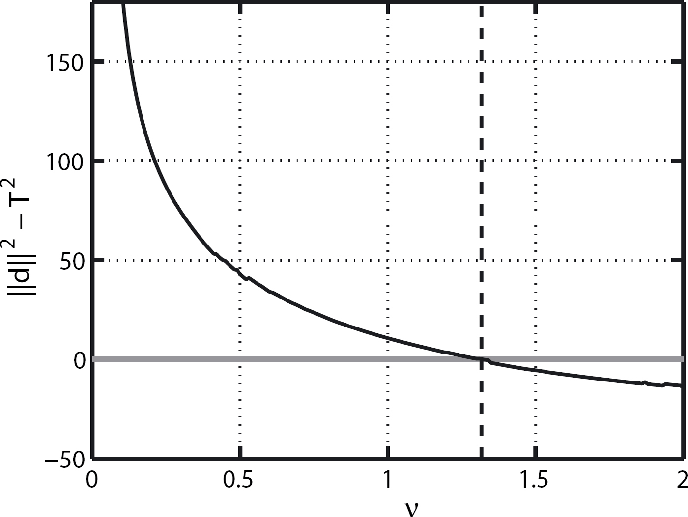
(section 4), shows how the data mismatch ‖ d‖2 typically varies with trade-off parameter v. When v is small, minimizing Ip with respect to the parameters (Equation (13)) overemphasizes model smoothness at the expense of a large data misfit ‖ d ‖ . When v is large, minimizing Ip overemphasizes data fit, making ‖ d‖2 very small at the expense of model smoothness, and (‖d‖ – T2) becomes negative; the data vector d (or the noise in the data) has been fit more closely than the data uncertainties can justify. This high degree of fit is achieved by the presence of extraneous structure in the solution vector p. For Taylor Mouth data, as shown in Figure 1, the model fits the data at the expected level T 2 for v =1.3, and the model-parameter vector p found when using this value of v is the preferred solution.
4. Taylor Mouth
To illustrate the solution of an inverse problem with this approach, we have found the spatial accumulation-rate pattern at Taylor Mouth, a site in Antarctica at the head of Taylor Valley (Fig. 2). Taylor Mouth is approximately 30 km northeast of the Taylor Dome ice-core site, where an ice core to bedrock was collected in 1994 (Reference Grootes and SteigGrootes and others, 1994). That core has provided a 150 kyr stable-isotope paleoclimate record (Reference SteigSteig and others, 2000; Reference Grootes, Steig, Stuiver, Waddington and MorseGrootes and others, 2001) and an atmospheric CO2 record for the past 60 kyr (Reference Indermuhle, Monnin, Stauffer and StockerIndermuhle and others, 2000). Several short (100 m) firn cores were also collected, in order to assess the spatial variability of climate, and climate-signal preservation in the area. One of these cores was collected from Taylor Mouth (Reference Neumann, Waddington and SteigNeumann and others, 2005).
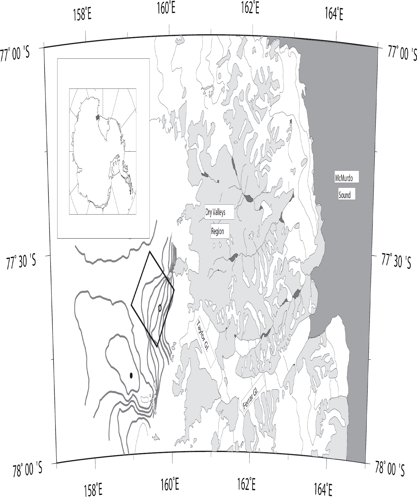
Fig. 2. Location of Taylor Dome. Solid dot marks location of 554 m Taylor Dome ice core. Surface-elevation contours were measured by airborne radar survey (Reference MenkeMorse, 1997). Box denotes Taylor Mouth study site, shown in Figure 3. Open circle marks 100 m core.
4.1. Observations and flowband
The ice at the Taylor Mouth core site (TM in Fig. 3) originates along a flowline from a saddle approximately 12 km to the northwest (Figs 2 and 3). Strong internal layers are visible in the radar profile (Fig. 4). The strain network shown in Figure 3 provided surface ice-velocity data. We surveyed the flow markers by optical methods tied to a local bedrock monument (on the nunatak near [49 km, 10 km] in Fig. 3), which had been tied to a reference GPS base station at

Fig. 3. Surface topography and ice flow of Taylor Mouth area. Local coordinate system is as described by Reference Morse and WaddingtonMorse and others (2007). Dots represent poles in strain grid used to infer surface ice-flow velocities and the flowband through the core site at TM. Stars denote locations of gross-ð accumulation and 10m firn-temperature measurements. Black area in lower right is a nunatak, to which velocity surveys were referenced.

Fig. 4. Ice-penetrating radar profile along Taylor Mouth flowband. Vertical bar marks the 100 m core hole. Bold solid curve marks the internal layer used as data in the inverse problem. (Apparent surface-parallel features in upper 50 m are an artifact.)
McMurdo Station, Antarctica, as described by Reference Morse and WaddingtonMorse and others (2007). We estimated the standard error of these velocity data to be ![]() . To find the flowline shown in Figure 3, we interpolated the velocity field between these measured markers. Starting at the core site and working both upstream and downstream, we tracked the locus of points that was everywhere parallel to the local velocity field. To find the relative flowband width W(x) shown in Figure 5d, we repeated the flowline calculation, starting from two points near the core site but offset several hundred meters in opposite directions transverse to the flow. The relative flowband width W(x) is the separation between these two flowlines, normalized by their separation at the core site.
. To find the flowline shown in Figure 3, we interpolated the velocity field between these measured markers. Starting at the core site and working both upstream and downstream, we tracked the locus of points that was everywhere parallel to the local velocity field. To find the relative flowband width W(x) shown in Figure 5d, we repeated the flowline calculation, starting from two points near the core site but offset several hundred meters in opposite directions transverse to the flow. The relative flowband width W(x) is the separation between these two flowlines, normalized by their separation at the core site.
We measured ice thickness along that central flowline with the University of Washington ice-penetrating radar system described by Reference WeertmanWeertman (1993) and Reference GadesGades (1998). This profile also includes internal layers (Fig. 4); we attribute a standard error of ![]() to the depth of the layer indicated by the dashed curve. We converted the radar travel times to depths using the known source–receiver separation, and wave speeds of 300 m µs∼1 in air for the direct wave, and 168 m µs∼1 in ice. After accounting for the two-way travel time through the ice and approximately 15 m of air in the firn, we recovered ice-equivalent depths.
to the depth of the layer indicated by the dashed curve. We converted the radar travel times to depths using the known source–receiver separation, and wave speeds of 300 m µs∼1 in air for the direct wave, and 168 m µs∼1 in ice. After accounting for the two-way travel time through the ice and approximately 15 m of air in the firn, we recovered ice-equivalent depths.

Fig. 5. (a) Accumulation-rate solution ![]() Gray band spans range of solutions associated with uncertainties in data as described in section 5.2. (b) Narrow triangles show locations and widths of a series of perturbations (amplitudes not to scale) that were added to individual nodes of the preferred accumulation-rate solution in (a). Each corresponding bold curve is a model-resolving function, which shows the ability of the inverse procedure to recover that perturbation. (c) Vertical section along flowband. End points of dotted particle paths define 1662 year layer (bold solid curve). Other modelled layers, at 500 year intervals, are shown by dashed and dotted subhorizontal curves. Other particle paths (solid curves) provide model ages for the ice core (bold vertical line). (d) Non-dimensional flow-band width W(x), inferred from surface topography and surface-velocity measurements (Fig. 3). (e) Positive surface curvature (concave topography) correlates with high accumulation rate, probably due to deceleration of both upslope and downslope winds.
Gray band spans range of solutions associated with uncertainties in data as described in section 5.2. (b) Narrow triangles show locations and widths of a series of perturbations (amplitudes not to scale) that were added to individual nodes of the preferred accumulation-rate solution in (a). Each corresponding bold curve is a model-resolving function, which shows the ability of the inverse procedure to recover that perturbation. (c) Vertical section along flowband. End points of dotted particle paths define 1662 year layer (bold solid curve). Other modelled layers, at 500 year intervals, are shown by dashed and dotted subhorizontal curves. Other particle paths (solid curves) provide model ages for the ice core (bold vertical line). (d) Non-dimensional flow-band width W(x), inferred from surface topography and surface-velocity measurements (Fig. 3). (e) Positive surface curvature (concave topography) correlates with high accumulation rate, probably due to deceleration of both upslope and downslope winds.
Surface elevations in Figure 3 were measured along 5 km gridlines as part of an airborne ice-penetrating radar survey with GPS control (Reference MenkeMorse, 1997). We also measured the surface-elevation profile shown in Figure 5c, with a ground-based continuous GPS survey along the flowline. The surface elevations are known to within ![]()
Reference Morse and WaddingtonMorse and others (1999) detected the radioactive horizons from above-ground bomb testing in the 1950s and 1960s (Reference Picciotto, Wilgain and snowPicciotto and Wilgain, 1963) using gross–β measurements on a shallow core. As a result of the low net accumulation rate at the Taylor Mouth core site (Fig. 5), these horizons are not well preserved, resulting in relatively low confidence (high uncertainty) in the accumulation-rate measurement. The average accumulation rate at the core site was b = 0.023 m a∼1, with ![]() over the four decades between 1955 and 1994.
over the four decades between 1955 and 1994.
4.2. Data for inverse problem
We used our inverse procedure to determine the accumulation rate at 60 nodes ![]() spaced at 200 m along the flowband through the Taylor Mouth core site. Our data comprised: the ice-surface profile (Fig. 5c); the uppermost continuous
spaced at 200 m along the flowband through the Taylor Mouth core site. Our data comprised: the ice-surface profile (Fig. 5c); the uppermost continuous
internal layer (highlighted in Fig. 4); the ice velocity measured at the core site and at three other sites along the flow-band (see Fig. 3); and the accumulation rate measured at the core site (TM in Fig. 3). The ice-surface data comprised elevations at the NS = 60 nodes x(n) spaced at 200 m, and the internal-layer data comprised measured depths at the ending x positions of 70 particle paths in the forward model (e.g. see Fig. 5c).
4.3. Site-specific simplifications
In section 3, we described the inversion procedure in very general form. We now select an appropriate thermomechanical ice-flow model for the Taylor Mouth flowband. This flow model should be as sophisticated as necessary to accurately represent the flow field as it impacts the targeted layer along this flowband, while being as simple as possible to facilitate the inversion procedure.
Thermomechanical calculations
At Taylor Mouth, we use horizontal-velocity shape functions ![]() based on the SIA (e.g. Reference PatersonPaterson, 1994, p.262), incorporating depth-varying temperature. Measured accumulation rates are only a few centimeters (ice equivalent) per year, so vertical velocities are small and advective heat transfer is unimportant. We calculate a 1-D vertical temperature profile θ(x, z) at each node
based on the SIA (e.g. Reference PatersonPaterson, 1994, p.262), incorporating depth-varying temperature. Measured accumulation rates are only a few centimeters (ice equivalent) per year, so vertical velocities are small and advective heat transfer is unimportant. We calculate a 1-D vertical temperature profile θ(x, z) at each node ![]() using the 1-D steady-state temperature model of Reference Firestone and WaddingtonFirestone and others (1990). By using the Taylor Dome value of geothermal flux (Table 1), in which we have high confidence, we decouple qgeo from the other model parameters. Since the basal temperature is below the melting point everywhere along the flowband, we set basal sliding u(x, 0) = 0 and basal melting
using the 1-D steady-state temperature model of Reference Firestone and WaddingtonFirestone and others (1990). By using the Taylor Dome value of geothermal flux (Table 1), in which we have high confidence, we decouple qgeo from the other model parameters. Since the basal temperature is below the melting point everywhere along the flowband, we set basal sliding u(x, 0) = 0 and basal melting ![]() =0 further simplifying the inverse problem. Details of our thermomechanical ice-flow calculations are provided in Appendix B.
=0 further simplifying the inverse problem. Details of our thermomechanical ice-flow calculations are provided in Appendix B.
Table 1. Expected values and solution characteristics for model parameters p j and trade-off parameter v. Ice flux q in is reported in m3 a− 1 per m width of flowband at the boundary. H 0 is the ice-equivalent thickness at the core site. Standard deviations of the solution were calculated from 100 parameter solutions derived from randomly perturbed datasets

Jacobian matrices
The matrices J
c
and J
r
of partial derivatives ∂ci/∂pj and ∂ri/∂pj in Equation (22) are straightforward to construct numerically, by perturbing each parameter pj in turn, and recalculating all the model residuals ci
and data residuals ri
with the forward thermomechanical model. However, this procedure is computationally intensive. Instead, we first note that the expressions for ci in Equations (15) and (16) can be differentiated directly. Then, noting that the residuals ri (Equation (18)) depend on the parameters pj only through the observables ![]() , we express each observable quantity
, we express each observable quantity ![]() as a function of the model parameters p so that we can find analytical expressions for these derivatives wherever possible. For example, the accumulation rate
as a function of the model parameters p so that we can find analytical expressions for these derivatives wherever possible. For example, the accumulation rate ![]() at any x can be interpolated from the bi model parameters. Ice flux q(x) can be related to p through Equation (2). Velocity u(x, S(x)) at the ice surface S(x) at any position x can be expressed in terms of the parameters by first expressing velocity in terms of flux q(x) using Equations (3) and (4).
at any x can be interpolated from the bi model parameters. Ice flux q(x) can be related to p through Equation (2). Velocity u(x, S(x)) at the ice surface S(x) at any position x can be expressed in terms of the parameters by first expressing velocity in terms of flux q(x) using Equations (3) and (4).
Surface-profile data
The modelled ice-surface profile S(m)(x) cannot be written readily as an analytical function of the model parameters, and as a result, the partial derivatives ∂S(m)(x(n))/∂pj need to be evaluated numerically. We avoided this computational cost by decoupling the ice-surface residuals from the other data, and at the same time decoupling the enhancement factor, E, from the other model parameters. E appears only in Equation (B8) (see Appendix B), where it is used to find the steady-state surface profile, S(m)(x), with a dynamic calculation. We chose to use the observed surface, S(d)(x), while finding values for all the other parameters, p, in the inversion process. After solving the inverse problem, we incorporated those solution parameters in Equation (B8), and adjusted E to minimize the mismatch between the modelled surface, S(m)(x), and the observed surface, S(d)(x). For our Taylor Mouth dataset, we were able to match the surface to within observational error, using E = 0.75. This internal consistency after the calculations were completed justifies decoupling E from the other model parameters.
For some other datasets, it may be more important to include E as a coupled model parameter throughout the inversion, and to include the observed surface topography, S(d)(x), as data to be matched at each iteration.
Model-parameter considerations
For this inverse solution, we assigned a characteristic length scale, L(c) = 700 m, which is comparable to the ice thickness, and a characteristic accumulation rate, ![]() which is comparable to the value at the core site. These values were used in Equation (15). We initially estimated the input flux, qin
, by extrapolating the flowband upstream to the ice divide, and applying
which is comparable to the value at the core site. These values were used in Equation (15). We initially estimated the input flux, qin
, by extrapolating the flowband upstream to the ice divide, and applying ![]() in that area. We initially estimated the layer age with the LLA, using the measured depth of the layer at the core site, and the average of
in that area. We initially estimated the layer age with the LLA, using the measured depth of the layer at the core site, and the average of ![]() and the measured accumulation rate at the core site. We attributed large acceptable deviations,
and the measured accumulation rate at the core site. We attributed large acceptable deviations, ![]() to these model parameters (see Equation (16), and Table 1). As a result, our preconceptions had only a small impact on the solution for q
in
, and A. In Table 1 we show expected values,
to these model parameters (see Equation (16), and Table 1). As a result, our preconceptions had only a small impact on the solution for q
in
, and A. In Table 1 we show expected values, ![]() and acceptable deviations,
and acceptable deviations, ![]() from those expectations for the model parameters q
in
, A, H
0
, E and q
geo
. Our site-specific simplifications allowed us to decouple H0, E and q
geo
from the main inverse problem, and thereby to significantly reduce computational time. In section 5.1, we show why this simplification was justified.
from those expectations for the model parameters q
in
, A, H
0
, E and q
geo
. Our site-specific simplifications allowed us to decouple H0, E and q
geo
from the main inverse problem, and thereby to significantly reduce computational time. In section 5.1, we show why this simplification was justified.
5. Results
5.1. Model parameters and predicted observables
We solved the non-linear system of Equation (13) for the range of values of v shown in Figure 1. The mismatch criterion Equation (11) is satisfied by v = 1.3; we accepted the accumulation-rate profile and other model parameters associated with v = 1.3.
Using the preferred value for the trade-off parameter, v = 1.3, we inferred the accumulation-rate profile in Figure 6a, shown before and after it evolved through successive iterations. The corresponding modelled internal-layer shapes are shown in Figure 6b. The final modelled layer agrees closely (but not too closely) with the observed layer. Table 2 shows how well the modelled observables match the data. In spite of the large observational uncertainty, the modelled accumulation rate at the core site exceeds the measured value from bomb fallout by more than ![]() Three of the four modeled surface velocities matched the measured velocities to within
Three of the four modeled surface velocities matched the measured velocities to within ![]() To estimate the standard deviations of the modelled observables in Table 2, we created 100 predictions of all observables using 100 realizations of the parameter solution, as described in section 5.2.
To estimate the standard deviations of the modelled observables in Table 2, we created 100 predictions of all observables using 100 realizations of the parameter solution, as described in section 5.2.

Fig. 6. (a) Model estimates of ![]() start from the LLA (thin solid curve), and converge to bold solid curve. (b) Corresponding modelled internal-layer shapes. Initial estimate (thin solid curve), found by using LLA-derived accumulation in (a) in forward algorithm, is a poor match to the observed layer (solid gray curve). Final modelled layer is shown by bold solid curve. (c) Distribution of nondimensional mismatches (Equation (18)) between observations and model, normalized to have unit integral. Resemblance to normal probability-density distribution (solid curve) confirms that Equation (20) defines appropriate tolerance level T.
start from the LLA (thin solid curve), and converge to bold solid curve. (b) Corresponding modelled internal-layer shapes. Initial estimate (thin solid curve), found by using LLA-derived accumulation in (a) in forward algorithm, is a poor match to the observed layer (solid gray curve). Final modelled layer is shown by bold solid curve. (c) Distribution of nondimensional mismatches (Equation (18)) between observations and model, normalized to have unit integral. Resemblance to normal probability-density distribution (solid curve) confirms that Equation (20) defines appropriate tolerance level T.
Figure 6c shows a histogram of the mismatches (70 points in the layer-depth profile, four surface velocity points, and accumulation at the core site), non-dimensionalized with the standard errors of the data. The histogram amplitudes are also normalized so that they integrate to unity. Because we incorporated the mismatch criterion Equation (11), the mismatches do approximate a set of samples from a probability-density distribution with zero mean and unit variance (thin solid curve in Fig. 6c), i.e. the model solution is a reasonable fit to the data.
The solution of the inverse problem also returned the age of the layer, A = 1662 years, and the ice flux entering the upstream end of the flowband, q
in
= 17.8 m3 a−1 per meter width of flowband. To assess the appropriateness of decoupling H0 and E from the other model parameters, we ran a series of dynamic steady-state forward models as described by Equation (B8) in Appendix B, and driven by our preferred solution for boundary flux, q
in
, and accumulation-rate profile, ![]() We varied the ice thickness, H0, at the core site and enhancement factor, E, in Equation (1), and for each pair we calculated the root-mean-square (rms) mismatch between the surface-profile data and the surface predicted by the forward calculation. Figure 7 shows that the surface profile from the dynamic flow model agreed with the measured surface to within 1 m (rms) for H0 = 647 m and E = 0.75. This finding confirms that if we had included H0 and E as model parameters in the general inverse procedure, we would have obtained E ≈ 1, in agreement with our expectations, and the other model parameters, p, would have been very similar to those that we actually obtained. Therefore, decoupling the surface topography calculation and the enhancement factor from the inverse problem was appropriate at Taylor Mouth.
We varied the ice thickness, H0, at the core site and enhancement factor, E, in Equation (1), and for each pair we calculated the root-mean-square (rms) mismatch between the surface-profile data and the surface predicted by the forward calculation. Figure 7 shows that the surface profile from the dynamic flow model agreed with the measured surface to within 1 m (rms) for H0 = 647 m and E = 0.75. This finding confirms that if we had included H0 and E as model parameters in the general inverse procedure, we would have obtained E ≈ 1, in agreement with our expectations, and the other model parameters, p, would have been very similar to those that we actually obtained. Therefore, decoupling the surface topography calculation and the enhancement factor from the inverse problem was appropriate at Taylor Mouth.

Fig. 7. Root-mean-square mismatch between observed surface topography and topography calculated with forward model (see Equation (B8) in Appendix B), for a range of ice thickness H0 at core site, and enhancement factor E, using qi
n
and ![]() parameters from preferred solution of the inverse problem in all cases. Minimum at H0 = 646 m and E = 0.75 suggests that if H0 and E had not been decoupled from the other parameters to simplify this particular inverse problem, values similar to these would have been obtained.
parameters from preferred solution of the inverse problem in all cases. Minimum at H0 = 646 m and E = 0.75 suggests that if H0 and E had not been decoupled from the other parameters to simplify this particular inverse problem, values similar to these would have been obtained.
5.2. Confidence limits on solution
Because of the standard errors associated with each observation, our dataset is just one realization out of an infinite number of possible realizations of the same set of observable quantities. In order to estimate uncertainties in the derived model-parameter vector p, we created 100 synthetic datasets, and derived a corresponding set of model parameters from each. We assumed that each observation ![]() of accumulation rate or velocity was independent of the other data. In each synthetic dataset, we replaced the accumulation-rate measurement and each velocity observation by a value selected at random from our estimate of its underlying normal probability-density distribution, defined by its mean (assumed to be its observed value
of accumulation rate or velocity was independent of the other data. In each synthetic dataset, we replaced the accumulation-rate measurement and each velocity observation by a value selected at random from our estimate of its underlying normal probability-density distribution, defined by its mean (assumed to be its observed value ![]() ) and its observational uncertainty
) and its observational uncertainty ![]() . We assumed that the observations of layer depth
. We assumed that the observations of layer depth ![]() were cross-correlated. We represented correlated noise among the layer-depth data using a red-noise process. A red-noise series f (x) can be generated by
were cross-correlated. We represented correlated noise among the layer-depth data using a red-noise process. A red-noise series f (x) can be generated by
where α describes the cross-correlation of the noise series at lag Δx, and σ is an amplitude scaling a random-noise series n(x), with zero mean and unit variance. To create each synthetic dataset, we added red noise to the observed layer-depth profile h(d)(x). We generated 100 red-noise series with Equation (23), using Δx = 200 m (the node separation) and a = 0.9866, which creates cross-correlation ‘memory’ over distances of several kilometers. We used σ = 5 m, which is also the uncertainty ![]() in the layer-depth measurements. After solving the inverse problem for each of these 100 synthetic datasets, we constructed a statistical representation of the solution, by finding the mean and standard deviation of each parameter pj
.
in the layer-depth measurements. After solving the inverse problem for each of these 100 synthetic datasets, we constructed a statistical representation of the solution, by finding the mean and standard deviation of each parameter pj
.
The gray band in Figure 5a shows our estimate of the uncertainty in our accumulation-rate solution, based on the spread of results from this suite of experiments with synthetic datasets. Clearly, the peak in accumulation rate near x = 4 km is a robust feature. The associated standard deviations in layer ages A and incoming ice flux q in are shown in Table 1.
5.3. Topography and accumulation rate
Reference King, Anderson, Vaughan, Mann and MobbsKing and others (2004) related accumulation-rate variations (at the scale of 1 km) to modelled wind speed and snow transport associated with subtle slope changes at Lyddan ice rise, Antarctica. Reference Vaughan, Corr and DoakeVaughan and others (1999) found a strong
correlation between accumulation rate and surface slope dS/dx on Fletcher Promontory, Antarctica, and Reference FrezzottiFrezzotti and others (2004, Reference Frezzotti, Urbini, Proposito and Scarchilli2007) also found a correlation between net accumulation rate and surface slope in East Antarctica. At Taylor Mouth, accumulation is also related to topography; however, we find a better correlation with surface curvature d2S/dx2. Highest accumulation occurs where the surface is concave (near x = 4 km in Fig. 5e). There, upslope winds encounter steepening slopes, and downslope winds encounter lessening slopes. In both cases, wind speed tends to decrease, and suspended and saltating snow tends to be deposited. This effect is probably widespread; Reference Leonard, Bell and StudingerLeonard and others (2004) found a region of high accumulation rate along the western shore of Subglacial Vostok Lake, Antarctica, where the surface is also concave upward.
5.4. Depth-age scale
Since the Taylor Mouth core is 100 m long, it is composed primarily of firn rather than ice. Because theflowband model uses ice-equivalent thickness, we converted the measured thickness along the flowband to ice-equivalent thickness H(x) using the density-depth profile θ(z) (Fig. 8), measured on the Taylor Mouth ice core. Near-surface density at the core site was also measured by M. Duval (personal communication) in a 2 m deep snow pit.

Fig. 8. Density variation with depth in the Taylor Mouth core, based on mass and volume measurements of core sections (data from P.M. Grootes and E.J. Steig).
We then used our accumulation-rate solution (Fig. 5a), together with the particle-tracking module described in section 2, to calculate the steady-state depth-age relationship (in ice equivalent) of the Taylor Mouth ice core. This depth-age estimate takes into account spatial variations in accumulation rate, ice thickness, and strain associated with flow upstream from the core site. Finally, we converted this depth– age relation back to true depth, using θ(z). This depth–age scale is shown by the solid white curve in Figure 9. The gray band shows the range of depth–age curves resulting from the range of solutions, p, that generated the gray band in Figure 5a.

Fig. 9. Estimates of Taylor Mouth depth-age scale. Bold dashed curve produced by 1-D flow algorithm (Equation (35)), using measured density of the core (Fig. 8), and measured accumulation rate (b = 0.023 ± 0.010 ma−1 ) at the core site (x = 11.2 km in Fig. 5). Gray region reflects uncertainty in measured b. Solid black curve and hatched area result from 1-D flow algorithm (section 6.6) using long-term accumulation rate at the core site (0.036 ± 0.009 ma−1) inferred from flowband inverse problem. Solid white curve is derived from accumulation-rate solution and particle paths in Figure 5. Gray band around it spans age predictions from the same 100 accumulation-rate profiles used to generate gray band in Figure 5a.
6. Discussion
6.1. Steady-state assumption
We assumed that ice flow at Taylor Mouth is in steady state. We used a time-dependent flowband model (not described here) to verify this assumption. Following a climate perturbation, ice flux in our time-dependent flow model relaxed with an e-folding time of approximately 5000 years. The climate at Taylor Dome has probably been relatively stable over the past 6000 years (Reference MorseMorse and others, 1998; Reference Steig, Hart, White, Cunningham and DavisSteig and others, 1998; Reference MorseMonnin and others, 2004), so ice-age transients have largely run their course, and therefore ice flow at Taylor Mouth is approximately in steady state.
Our steady-state forward ice-flow model, when run with the accumulation-rate solution (Fig. 5a), also matches the shapes of deeper layers, although, as might be expected, with a somewhat higher standard deviation (^10 m) than we find for the layer that we used in the inverse problem. We also obtained solutions for (assumed) steady accumulation-rate profiles by repeating the inversion process, using several successively deeper layers with ages up to 2700 years in the solutions. These accumulation-rate solutions had magnitudes and structure similar to the solution in Figure 5a. These results suggest that our assumption of steady-state thickness and flow is reasonable, over millennial timescales.
6.2. Millennial accumulation patterns
Accumulation rates derived from near-surface internal layers by the SLA are necessarily short-term averages (e.g. ∼10– 100 year averages). Since accumulation rates in the polar regions are influenced by multi-annual (El Niño-Southern Oscillation (ENSO), e.g. Reference Bromwich and MonaghanBromwich and others, 2004) to multi-decadal atmospheric cycles (Arctic/Antarctic Oscillations, e.g. Reference Appenzeller and StockerAppenzeller and others, 1998; Reference Noone and SimmondsNoone and Simmonds, 2002), short-term accumulation rates may not be applicable over longer timescales, and should be used with caution in ice-flow studies. Our formal inverse-problem approach allows deeper (and therefore older) internal layers to be used to determine longer-term average accumulation rates.
Our geophysical-inverse approach assumes that accumulation rate is constant in time, and that ice flow is steady. For deep layers that pre-date the relative stability of the late Holocene, these may be questionable assumptions. It should be possible to relax these two model assumptions independently. We could determine the accumulation-rate pattern at different times in the past by using multiple layers in the inverse procedure. In addition, replacing Equation (B8) with a transient continuity equation (e.g. Reference PatersonPaterson, 1994, p. 322) would also allow for changes in ice thickness along the flow-band as a function of time.
6.3. Response to incompatible data
The inversion procedure assumes steady-state accumulation and flow, and expects the data to represent long-term average values of the observable quantities. Ice-sheet thickness and velocity change slowly, and are insensitive to decadal or centennial fluctuations in accumulation rate, because of the 5000 year response time. It takes a long time for accumulation variations to build up thicker ice or steeper slopes, and these slow changes control velocity changes. Although we obtained our velocity and ice-thickness data over a period of only a few years, we can expect those data to be representative of behavior on a millennial timescale.
In contrast, accumulation rate can change rapidly (Reference Van der VeenVan der Veen, 1993; Reference McConnellMcConnell and others, 2000). The inversion procedure can inform us how well observations represent long-term averages. One of the larger mismatches (w1.5σ) among all our data points (see Table 2) occurred for the measured accumulation rate at the Taylor Mouth core site. The measured value (0.023 ± 0.01 ma−1), using bomb radioactivity, represents an average over approximately 40 years. This value is less than two-thirds of the solution of 0.036 ± 0.009 m a−1 in Figure 5a, which provides an average value over 1662 years.
Table 2. Data and modelled observables. Standard deviations of modelled observables were calculated from 100 sets of data predictions using 100 parameter solutions derived from randomly perturbed datasets

This large mismatch suggests that the accumulation rate between 1955 and 1995 was significantly lower than the millennial average. Reference Morse and WaddingtonMorse and others (1999) used gross-,0 activity in bomb layers to measure accumulation rate at a second site (607 in Fig. 3). Because site 607 lies 2 km from the flowline, we did not use its accumulation-rate data (0.051 ± 0.005 ma−1) when solving the inverse problem. However, the ‘bowl’ shape of the Taylor Mouth catchment (Fig. 3) tends to funnel katabatic flow, so it is reasonable to expect that accumulation rate at any given time varies primarily in the downslope direction, and is relatively uniform along the contours over short distances where the slopes do not vary significantly. Site 607 projects along the 2250 m contour onto the flowband at x = 5.5 km, where our solution (Fig. 5a) finds a larger accumulation rate of 0.070 ± 0.006 m a−1.
At both site 607 and the core site, the millennial value of accumulation rate is approximately 50% larger than the measurements from 1955 to 1994, indicating that the late 20th century was probably relatively dry throughout the Taylor Mouth area.
Measurements of cosmogenic 10Be also suggest that the accumulation rate derived from bomb layers was lower than the long-term average. Over timescales longer than the 11 year sunspot cycle, 10Be is often assumed to fall out at a constant rate. Because snow dilutes the 10Be, the concentration of 10Be should be inversely proportional to the accumulation rate. Reference SteigSteig (1996) measured the average concentration of 10Be at Taylor Mouth in the upper 5 m, which spans approximately 80 years. On the basis of those measurements, Reference Morse and WaddingtonMorse and others (1999) reported an average accumulation rate of 0.0395 m a−1 at the Taylor Mouth core site. This value is indistinguishable from our millennial average of 0.036 ± 0.004 m a−1, suggesting that, if the late 20th century was dry in the Taylor Mouth basin, then the early 20th century had compensating above-average snowfall.
While technically reliable, the gross-0 measurement of accumulation rate at the Taylor Mouth core site was not a good measure of the quantity that the inversion procedure expected it to represent, i.e. an accumulation rate over the past 1662 years. Because of our steady-state assumption and the inherent short-term variability of accumulation, this data point was incompatible with the other data, which better represented conditions averaged over a millennium. As a result of this incompatibility, the inversion procedure was unable to fit this data point closely. Reference Baldwin, Bamber and PayneBaldwin and others (2003) also noted systematic differences between short-term surface measurements of accumulation rate, and long-term values inferred from internal layers in Greenland.
6.4. Resolving power
Before making physical inferences from our preferred solution, it is important to assess the resolving power of the model. The model size is defined in section 3.3 through a smoothness condition on the accumulation-rate profile (Equation (15)). As outlined in section 3.1, this smoothness condition regularizes the model, and prevents spurious detailed structures from appearing in the model solution. It can also limit our ability to resolve real structures at fine spatial scales. Reference ParkerParker (1994) showed that, in a regularized model,
the true solution has been smoothed by a set of narrowly peaked resolving functions. These model-resolving functions indicate how closely the preferred solution is able to reproduce detailed structure in the underlying ‘true’ solution.
Following Reference ParkerParker (1994) and Reference TrufferTruffer (2004), we can calculate the model-resolving function for each model parameter in our preferred solution, which we will call p0. Using p0 in the forward algorithm produces a synthetic dataset ![]() . Because the solution procedure does not fit the data exactly (see Equation (11)), this dataset
. Because the solution procedure does not fit the data exactly (see Equation (11)), this dataset ![]() and the actual measured dataset o(d) can be viewed as two equivalent realizations of the same underlying observables, and their differences r (see Equation (18)) are distributed across all dimensions of the data space. If we then solve the inverse problem using
and the actual measured dataset o(d) can be viewed as two equivalent realizations of the same underlying observables, and their differences r (see Equation (18)) are distributed across all dimensions of the data space. If we then solve the inverse problem using ![]() as the data, we recover a new set of model parameters
as the data, we recover a new set of model parameters ![]() (‘rec’ for recovered). Because p0 and
(‘rec’ for recovered). Because p0 and ![]() are recovered from equivalent realizations of the data, their difference (
are recovered from equivalent realizations of the data, their difference (![]() – p0) should be small, and distributed across all the model parameters. Their rms difference shows the level of uncertainty that we can expect in general in the solution.
– p0) should be small, and distributed across all the model parameters. Their rms difference shows the level of uncertainty that we can expect in general in the solution.
Next we perturb in turn each model parameter pj
in the preferred solution p0, producing a perturbed vector of model parameters that we call p(j)). We then run the forward model using each pj to generate a perturbed set of observables ![]() . Using these calculated observables as new data
. Using these calculated observables as new data ![]() we then solve the new inverse problem to recover a new vector of parameters
we then solve the new inverse problem to recover a new vector of parameters ![]() , using the trade-off parameter v from the preferred model solution. The question of interest is how well we were able to recover the original perturbation to parameter pj.
, using the trade-off parameter v from the preferred model solution. The question of interest is how well we were able to recover the original perturbation to parameter pj.
We cannot just subtract each new solution ![]() from our original preferred (and unperturbed) solution p0, because the small random differences (
from our original preferred (and unperturbed) solution p0, because the small random differences (![]() −po would confound the quest to isolate the recovered image of the perturbation. We eliminate that confounding effect by forming the difference
−po would confound the quest to isolate the recovered image of the perturbation. We eliminate that confounding effect by forming the difference ![]() −
− ![]() to produce an image of the original impulsive perturbation to the corresponding model parameter pj. This image is the model-resolving function for that model parameter. We would like to be able to recover that impulsive perturbation exactly; invariably, however, some information is lost. In general, the resolving functions also have non-zero amplitudes at other parameters. When the parameter pj is part of a spatial sequence (e.g. accumulation-rate parameters
to produce an image of the original impulsive perturbation to the corresponding model parameter pj. This image is the model-resolving function for that model parameter. We would like to be able to recover that impulsive perturbation exactly; invariably, however, some information is lost. In general, the resolving functions also have non-zero amplitudes at other parameters. When the parameter pj is part of a spatial sequence (e.g. accumulation-rate parameters ![]() ), its resolving function tends to display a broadened peak involving other nearby model parameters. The width of each resolving function gives a physical scale of meaningful structure that can be resolved in the inverse problem. Steep gradients in true accumulation rates will appear as spread-out gentler gradients if they are limited to length scales shorter than the width of the resolving function.
), its resolving function tends to display a broadened peak involving other nearby model parameters. The width of each resolving function gives a physical scale of meaningful structure that can be resolved in the inverse problem. Steep gradients in true accumulation rates will appear as spread-out gentler gradients if they are limited to length scales shorter than the width of the resolving function.
Narrow triangles in Figure 5b show perturbations added to individual nodes of the preferred accumulation-rate solution in Figure 5a. The corresponding bold curves are the model-resolving functions, which demonstrate the ability of the inverse procedure to recover details about accumulation rate at a single node. The width of the resolving function increases with distance along the flowband, because ice velocity increases with distance from the divide, and ice particles that comprise the target layer travel longer distances and can experience larger ranges of accumulation rate and strain. This indicates that further from the divide a layer retains less information about short-scale spatial variability in accumulation; therefore our ability to discern such spatial variability decreases with distance from the divide. However, our preferred accumulation-rate solution shows major variations on spatial scales larger than the half-width spread of the resolving functions (of 1–2 km). Although only weighted mean values of accumulation rate can be resolved on length scales shorter than the resolving functions, the variations in our solution accurately reflect real trends over length scales of several kilometers.
Similarly, we can create data-resolving functions, by perturbing each data value in o(d) in turn, to create new datasets ![]() . Then we solve the inverse problem using each new dataset
. Then we solve the inverse problem using each new dataset ![]() in turn to find new model-parameter solutions p. Finally, we run the forward model with each new parameter set p in turn, to generate associated sets of observables o(m). Subtracting each new set of observables o(m) from our original (and unperturbed) dataset o(d) produces an image of the impulsive perturbation to the corresponding data value; this image is the data-resolving function for that observation. Each data-resolving function represents the degree to which that individual observable (data value) contributes unique information to the inverse procedure. Our data-resolution functions have widths comparable to those of the model-resolution functions. They also broaden in the downstream direction, indicating that useful information for the inverse problem is provided by progressively broader weighted averages of layer depth.
in turn to find new model-parameter solutions p. Finally, we run the forward model with each new parameter set p in turn, to generate associated sets of observables o(m). Subtracting each new set of observables o(m) from our original (and unperturbed) dataset o(d) produces an image of the impulsive perturbation to the corresponding data value; this image is the data-resolving function for that observation. Each data-resolving function represents the degree to which that individual observable (data value) contributes unique information to the inverse procedure. Our data-resolution functions have widths comparable to those of the model-resolution functions. They also broaden in the downstream direction, indicating that useful information for the inverse problem is provided by progressively broader weighted averages of layer depth.
6.5. Strain regimes and choice of forward algorithm
Before attempting to extract accumulation-rate information from a particular layer, we must determine the appropriate level of complexity required in the thermomechanical forward algorithm. For any layer, we can distinguish three situations, based on the impact of vertical strain on the depth of the layer, and on the impact of gradients of strain and accumulation rate along particle paths that reach the layer.
Shallow-layer approximation (SLA)
For accumulation rate ![]() and ice thickness H, a characteristic vertical strain rate is given by
and ice thickness H, a characteristic vertical strain rate is given by ![]() After we accountforfirn compaction, very shallow layers with depth h and age A have experienced almost no cumulative dynamic strain e associated with ice flow, if
After we accountforfirn compaction, very shallow layers with depth h and age A have experienced almost no cumulative dynamic strain e associated with ice flow, if
Consequently, accumulation can be estimated locally from layer depth and age, through
Combining Equations (24) and (25) shows that this approximation is valid only when h/H ≪1 (e.g. in the upper few meters of a valley glacier, or in the upper 10–20 m (ice equivalent) of a thick ice sheet). The largest contributor to uncertainty can be imperfect knowledge of the density variation with depth. Reference Pinglot, Hagen, Melvold and EikenPinglot and others (2001) used this approach for very shallow layers.
Local-layer approximation (LLA)
Where layers from several decameters depth or deeper are observed, the SLA (Equation (25)) cannot be used, because significant dynamic vertical strain has accumulated. Corrections based on a 1-D flow model are often applied at each site to account for vertical strain, i.e. the local vertical strain is used to approximate the strain encountered along an actual particle path. For example, if, following Reference Morse and WaddingtonMorse and others (1999), we assume that the vertical velocity w(z) is approximately linear with depth, such that the characteristic vertical strain rate e c h ar applies at all depths, then
which leads to the improved approximation

When a local 1-D or sandwich model (Reference ReehReeh, 1989) is used to make a strain correction, we call that process the LLA. For example, the LLA was used by Reference Morse and WaddingtonMorse and others (1999), Reference Fahnestock, Abdalati and LuoFahnestock and others (2001), Reference Kanagaratnam, Gogineni and GundestrupKanagaratnam and others (2001) and Reference Leysinger Vieli, Siegert and PayneLeysinger Vieli and others (2004).
Deep layers
We consider a layer to be ‘deep’ when the LLA is no longer applicable. For near-surface layers, the LLA may be as effective as the full inverse procedure that we have presented here, and less computationally intensive. For deeper layers, however, two effects warrant the use of a higher-dimensional inverse model.
First, in steady state, the downward ice velocity depends strongly on the local accumulation rate. Therefore, the depth of the layer at a particular point is a function of the average accumulation rate along the particle path, from its point of origin on the surface to the point where it intersects the measured layer (Fig. 5c). As the depth to an internal layer increases, a particle path is more likely to traverse regions of higher or lower accumulation rate, where the downward velocity pushes the path to a deeper or shallower trajectory, when compared with a path through a region of uniform accumulation rate. If the accumulation rate varies slowly with position, ice can follow a very long particle path, while still reaching a depth consistent with the LLA, based on the local accumulation rate at the end point. On the other hand, if the accumulation-rate gradient is large (as at Taylor Mouth), even moderate ice-flow velocities will cause internal-layer depths to differ significantly from the depth predicted with the LLA.
Second, as the depth of an internal layer increases to a larger fraction of the total ice thickness, the ice above that layer can be subjected to a greater total strain as a result of ice flow. Spatial variations of total vertical strain alter the depth of a layer, independent of the local accumulation rate, as demonstrated by Reference Hindmarsh, Siegert and GudmundssonHindmarsh and others (2002). Variations in strain are commonly associated with spatial gradients in ice thickness. Large thickness gradients along a particle path can have a strong influence on layer depth at the end point of that path.
To decide whether horizontal gradients are important, we compare the total length L path of a particle path, to characteristic lengths, L b· and LH , associated with accumulation-rate and ice-thickness gradients, respectively. We express the particle-path length as
where Ū is the temporally averaged horizontal velocity of a particle as it follows a particle path, and A is the age of the layer. A characteristic length Lb, associated with the accumulation-rate gradient, is the length over which b changes by an appreciable fraction:
Similarly, a characteristic length LH associated with the ice-thickness gradient is the length over which ice thickness changes by an appreciable fraction:
When several processes act simultaneously or sequentially to modify a quantity of interest such as layer depth, we also want to characterize their combined effects. One way to do this is to combine characteristic numbers that represent each process individually, in ways that reflect the nature of those interactions. If the characteristic numbers describe difficulty in achieving an effect, or resistance to a process, they can be combined as serial and parallel resistors in a network, the total resistance of which is the characteristic value that we seek. This approach is used to study rates of aerosol deposition to environmental surfaces such as snow (e.g. Reference DavidsonDavidson, 1989). Reference Waddington and SteigWaddington and others (2002) used this approach to explore the stability of stable-isotope ratios in polar snow. For our current question, a large characteristic length suggests that the depth to the internal layer varies slowly, so these characteristic lengths can be viewed as resistances to layer-depth variations. Because accumulation gradients and ice-thickness gradients act simultaneously, we can combine resistances ![]() and L
H in parallel to create a characteristic length scale Lδh
, which represents total resistance to layer-depth variations from the combined effects of accumulation gradients and ice-thickness gradients:
and L
H in parallel to create a characteristic length scale Lδh
, which represents total resistance to layer-depth variations from the combined effects of accumulation gradients and ice-thickness gradients:
We now compare L path to Lδh , to generate a non-dimensional number D:
If D ≪1, then spatial gradients in ![]() and H do not significantly impact layer depth, and the LLA can be used. However, if D > 1, then layer depth at a point is not necessarily directly related to accumulation rate at that point, and a more sophisticated approach should be used. At Taylor Mouth, both
and H do not significantly impact layer depth, and the LLA can be used. However, if D > 1, then layer depth at a point is not necessarily directly related to accumulation rate at that point, and a more sophisticated approach should be used. At Taylor Mouth, both ![]() and LH are important, and D ∼ 1 for the layer that we used. This conclusion is confirmed by the differences between the initial and final accumulation rate and modelled layer (Fig. 6). Clearly the initial guess, which was the LLA, was inadequate, and a deep-layer treatment is required.
and LH are important, and D ∼ 1 for the layer that we used. This conclusion is confirmed by the differences between the initial and final accumulation rate and modelled layer (Fig. 6). Clearly the initial guess, which was the LLA, was inadequate, and a deep-layer treatment is required.
6.6. Application to depth-age scales
Whenever the LLA is inadequate to infer accumulation rate from a layer, use of a 1-D modelling approach to produce a depth-age scale for a core to similar depth is also questionable. We illustrate this point by comparing two depth-age scales for the Taylor Mouth core. The first is produced by our flowband model, while the second is produced by the following 1-D flow model.
A 1-D flow model
The depth-age relationship A(z) for a firn core can be estimated from the measured density profile p(z) in the core if we make simplifying assumptions:
1. Firn compaction is a steady-state process that follows Sorge’s law (Reference PatersonPaterson, 1994, p. 14):
2. The downward velocity w(S) at the surface is equal to the net accumulation rate of snow at the site.
3. The accumulation rate is constant and uniform, i.e. independent of t, x and y.
Then conservation of mass, ∇ (pv) = 0, yields
where ![]() = (∂u/∂x) + (∂v/∂y) is the horizontal strain rate, which we assume is independent of depth over the length of the core, because horizontal velocity generally changes very little in the upper 20% of the ice column. Equation (34) can be integrated numerically from the surface, where w(S) is known, to yield the vertical-velocity profile w(z).
= (∂u/∂x) + (∂v/∂y) is the horizontal strain rate, which we assume is independent of depth over the length of the core, because horizontal velocity generally changes very little in the upper 20% of the ice column. Equation (34) can be integrated numerically from the surface, where w(S) is known, to yield the vertical-velocity profile w(z).
A second vertical integration,
produces an estimate of the depth-age scale A(z) for the core. This analysis assumes that the area around the Taylor Mouth core site is horizontal. An identical analysis can be carried out for a sloping surface and a surface-normal core by rotating the coordinate system accordingly. Because the surface slope at Taylor Mouth is small (∼0.02), accountingfor non-orthogonality of the surface and the core hole changed our calculated vertical velocity by <0.1%.
From repeated position measurements of the network of poles shown in Figure 3, the horizontal strain rate, ![]() , at the core site was determined to be 1.2 x 10⁻⁴a−1. The depth-age scale derived from the 1-D compaction model with the measured accumulation rate at the core site (0.023± 0.010 m a−1) is shown by the bold dashed black curve and the broad gray zone in Figure 9. This 1-D model can provide ages only down to the depth (60 m) at which the density of the core reaches the density of ice; the predicted age at 60 m is 2700 ± 900 years. When we repeated the calculation with
, at the core site was determined to be 1.2 x 10⁻⁴a−1. The depth-age scale derived from the 1-D compaction model with the measured accumulation rate at the core site (0.023± 0.010 m a−1) is shown by the bold dashed black curve and the broad gray zone in Figure 9. This 1-D model can provide ages only down to the depth (60 m) at which the density of the core reaches the density of ice; the predicted age at 60 m is 2700 ± 900 years. When we repeated the calculation with ![]() varied by ±10%, the calculated age varied by ±75 years at 60 m depth. Clearly, uncertainty in the accumulation measurement is the major contributor to uncertainty in depth-age, when using this 1-D model.
varied by ±10%, the calculated age varied by ±75 years at 60 m depth. Clearly, uncertainty in the accumulation measurement is the major contributor to uncertainty in depth-age, when using this 1-D model.
Comparison with flowband model These results would form our best estimate of the depth-age scale, if we had no additional information from other locations along the flowline. However, the bold solid black curve and the associated hatched zone show the range of depth-age scales from the 1-D compaction model when we used this 1-D model together with our new estimate of 0.036 ± 0.009 ma−1 (from Fig. 5a) for the 1662 year average accumulation rate at the core site. This calculation produced an age of 1610 (+620, -350) years at 60 m depth.
The 1-D model in Equation (35) is attractive in its simplicity. However, it cannot recognize the incompatibility of the measured (short-term) accumulation rate at the core site with respect to our (long-term) problem formulation (see section 6.3). As a result, it produced an error in age of 1090 years, or 68%, at 60 m depth, when using the measured accumulation rate, rather than the inferred long-term accumulation rate at the site. In addition, the 1-D model took into account environmental conditions only at the core site. This model may yield reasonable estimates for short cores from environments with low spatial gradients of accumulation rate. Longer cores contain ice that originated some distance upstream, and this ice may have experienced different climate and flow conditions. The same criterion D ≪ 1 (see Equation (32)) with which we assessed the validity of the LLA can also be used to assess the validity of a 1-D flow model applied to ice-core dating.
We also calculated a depth-age relationship (solid white curve in Fig. 9) for the core using the inferred accumulation-rate profile (Fig. 5a) in our forward Taylor Mouth flowband model, and finding travel times of particles on paths that terminated at the core. As expected, both 1 –D and 2-D models predict the same slope of the depth-age scale A(z) near the surface when both models use accumulation rates from Figure 5a. However, the two estimates diverge with depth, since A(z) from the flowband model incorporates upstream variations in accumulation rate and vertical strain. Since the accumulation rate increases upstream from the core site, the flowband model puts thicker layers in the upper 60 m and therefore puts younger ice at 60 m depth, where the two depth-age scales differ by 300 years, or approximately 18%.
Because the flowband model can exploit all data contained in the layer geometry to constrain accumulation rate, its error limits on depth-age are smaller than those for the 1-D model. This analysis confirms our expectation, based on the non-dimensional analysis in section 6.5, that the depth-age scale from the flowband model must be used for the Taylor Mouth ice core. More generally, the analysis confirms our expectation that non-dimensional analysis can determine whether a 1 -D approach to calculation of a depth-age scale is valid or not for ice at any desired depth at any ice-core site.
7. Conclusions
Internal layers in polar ice sheets contain the only remaining detailed record of past accumulation rates; however, recovering that information requires integrated application of a thermomechanical ice-flow algorithm and formal inverse methods. The depths of near-surface layers in an ice sheet can provide a direct measurement of accumulation rate using the SLA, because they require neither complicated strain corrections nor knowledge of the total ice thickness. However, shallow layers can provide average accumulation rate only over short timescales in the recent past. For deeper, older layers for which vertical strain is appreciable, a local strain correction can be applied to derive an accumulation-rate profile using the LLA. When internal-layer depths have been affected significantly by spatially variable ice strain and accumulation rate along particle trajectories, the LLA can be inadequate. The non-dimensional number, D, in Equation (32) determines when the LLA can be used, and when the full flowband particle-path treatment for deep layers is required. The same non-dimensional analysis can determine when a depth-age scale for an ice core can be derived with a 1-D analysis, and when spatial gradients of accumulation rate and ice thickness necessitate a full deep-layer treatment, with a 2-D or 3-D thermomechanical ice-flow algorithm.
When a deep-layer treatment is required, recovering the spatial pattern of accumulation rate should be posed as an inverse problem. We describe a general and versatile framework that incorporates a thermomechanical ice-flow algorithm to solve the forward problem, and uses radar data from a deep layer, together with other available data, including surface velocity, or accumulation-rate measurements in order to find a smooth accumulation-rate profile. Our procedure achieves an objective trade-off between solution smoothness and data fit, to avoid over-fitting the data.
To solve an inverse problem, we must solve the associated forward problem hundreds to thousands of times. To reduce computational time, the procedure used to solve the inverse problem should have the flexibility to make simplifications as necessary, while still capturing the essential physics of flow at each site. By describing ice velocities and particle paths in kinematic terms (see section 2.4), our approach offers the flexibility to choose the simplest thermomechanical ice-flow model for each problem. Simplifications can include force-balance approximations such as the SIA; decoupling of the thermal and mechanical forward calculations; isolation of model parameters that are not strongly coupled to the other model parameters, or that are independently well known; and isolation of datasets that can be matched readily using the partial model-parameter solution for other model parameters.
Although it spans less than the upper 20% of the ice depth, the depth-age scale for the Taylor Mouth ice core is significantly affected by regions of relatively high accumulation rate upstream from the core site. That region of high accumulation correlates with a region of concave surface topography, in which both upslope and downslope wind speeds might be expected to decrease, dropping suspended and saltating snow.
In future work, the next step is to simultaneously infer both ice-sheet surface evolution and changing accumulation-rate patterns over time, by assimilating a series of both deep and shallow layers, using an objective trade-off criterion (Equation (11)). There is much still to be learned about our ability to resolve model parameters, and to assess the utility of the various data, as described in section 6.4, for the long-term transient case.
Acknowledgements
We thank Antarctic Support Associates for field logistical support; J. Dibb, for gross-β, accumulation-rate measurements; M. Duval, for density measurements in snow pits; and P.M. Grootes and E.J. Steig, for density measurements on the Taylor Mouth core. H.C. Steen-Larsen contributed valuable insights on inverse problems. Reviewers F. Parrenin and D. MacAyeal, and Scientific Editor J. Meyssonnier provided many helpful comments and suggestions. This work was supported by US National Science Foundation grants OPP-8915924, OPP-9421644 and OPP-0440666.
Appendix A: Least-Squares Solution Procedure
Using Equations (17) and (19), the performance index in Equation (12) can be written as

where Np is the number of model parameters, and ![]() is the total number of data, comprising the layer-depth profile, surface-elevation profile, and any available measurements of accumulation rate and surface velocity. The positive weights
is the total number of data, comprising the layer-depth profile, surface-elevation profile, and any available measurements of accumulation rate and surface velocity. The positive weights ![]() are all equal to the trade-off parameter ν The goal is to find a vector of parameters pj that minimize Ip
for a given value of ν. The model residuals ci depend on the model parameters pj
, through Equations (15) and (16), and the data residuals ri depend on the model parameters pj, through the model predictions
are all equal to the trade-off parameter ν The goal is to find a vector of parameters pj that minimize Ip
for a given value of ν. The model residuals ci depend on the model parameters pj
, through Equations (15) and (16), and the data residuals ri depend on the model parameters pj, through the model predictions ![]() of observable quantities in Equation (18). Starting from estimates
of observable quantities in Equation (18). Starting from estimates ![]() of the parameters, we calculate trial values
of the parameters, we calculate trial values ![]() of the model residuals and
of the model residuals and ![]() of the data residuals. These values, when substituted into Equation (A1) along with an estimate ν(0) of the trade-off parameter, are unlikely to produce a minimum in Ip
. However, we can approximate the unknown values of the model residuals ci
and data residuals ri
that would minimize Ip
with ν = ν(0) by expanding ci and ri in the vicinity of their current estimates,
of the data residuals. These values, when substituted into Equation (A1) along with an estimate ν(0) of the trade-off parameter, are unlikely to produce a minimum in Ip
. However, we can approximate the unknown values of the model residuals ci
and data residuals ri
that would minimize Ip
with ν = ν(0) by expanding ci and ri in the vicinity of their current estimates, ![]() and
and ![]() :
:

Substituting Equation (A2) into Equation (A1) produces

Because model residuals ci and data residuals ri appear in similar forms, we can simplify the notation by combining them into a single column vector e
We also introduce the Np × Np
diagonal weight matrix W
c
, whose ith diagonal element is ![]() , and the N
d
× N
d
diagonal weight matrix W
r
, whose ith diagonal element is
, and the N
d
× N
d
diagonal weight matrix W
r
, whose ith diagonal element is ![]() =v1/2
. We can then form a (N
p
+ N
d
) × (N
p
+ N
d
) diagonal weight matrix
=v1/2
. We can then form a (N
p
+ N
d
) × (N
p
+ N
d
) diagonal weight matrix
Finally, we form a Np ×Np Jacobian matrix J c , whose element in row i and column j is the partial derivative ∂ci/∂pj, and a Nd × Np Jacobian matrix J r , whose element in row i and column j is the partial derivative ∂ri/∂pj. From these two matrices we form a global (N p + N d ) × N p Jacobian matrix, J:
The minimization Equation (13) becomes:
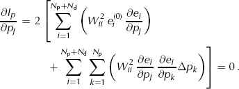
We can now express the complete set of these Np so-called normal equations for the least-squares solution in the matrix form
the solution of which is
Defining a (N p + N d ) × Np matrix A = WJ, and a column vector b = We, of length (Np + Nd), we can express Equation (A8) as
which has the standard form of the normal equations of the least-squares problem of finding the vector Δp that minimizes the quadratic form |AΔp — b|2 (e.g. Reference Press, Flannery and TeukolskyPress and others, 1986, p. 512).
However, the solution expressed in the form of Equation (A9) can be unstable or non-existent, if the matrix AT A = JTWT WJ is near-singular or singular. To avoid this problem, we use the singular value decomposition (SVD; e.g. Reference Press, Flannery and TeukolskyPress and others, 1986, p. 52) of matrix A, which in its reduced form is
where V is a N p × N p matrix whose columns V( ij ) (i = 1,…, N p ), are orthonormal basis vectors that span the N p -dimensional parameter space of all possible vectors Δp. The vector b exists in a (N p + N d )-dimensional space of residuals. However, the matrix A, by multiplying any vector Δp, can produce only vectors b that lie within an Np-dimensional sub-space known as the range of A. The columns U( i ), (i = 1,…, N p ) of the non-square (N p + N d ) × N p matrix U are orthonormal basis vectors that span the range of A within that (Np + Nd )-dimensional residuals space. Finally, Λ is a N p × N p diagonal matrix whose diagonal elements Xu are called the singular values, which are also the square roots of the eigenvalues of AT A.
Because columns of U and V are orthonormal, UT U and VT V produce identity matrices, and because Λ is diagonal, ΛT = Λ, and its inverse Λ−1 is also a N p × N p diagonal matrix, with 1/Λ ii as the ith diagonal element. With these simplifications, Equation (A8) reduces to
and the solution Equation (A9) reduces to
The N p × (N p + N d ) matrix [VΛ−1 UT ] is known as the generalized inverse of the (N p + N d) × N p matrix A = WJ.
SVD helps us to find a solution when ATA is ill-conditioned. Equation (A12) defining the problem can also be written in terms of the basis vectors U(i) and V(i) as

When the vector e (representing the known model residuals and data residuals) is written as a linear combination of the basis vectors U(i) spanning the range of A in the residuals space, the coefficient of each U(i) is given by the projection v(i) · Δp of the parameter-correction vector onto the corresponding ith basis vector in the parameter space, weighted by the ith singular value. If any parameter-change vector Δp lies entirely along a particular V(I), then the residual vector that it produces lies entirely along ui in the residuals space. If the weight Xii is small, then the component of Δp aligned with the corresponding basis vector V(i) has very little influence on the residual vector e, in the sense that the matrix A maps it onto some very small vector b. When the physical processes in the forward algorithm (represented by A) are integrative or diffusive, the basis vectors V(i) associated with small Λii tend to be highly oscillatory, and the oscillations tend to cancel when VI is mapped to the residuals space by A.
The solution vector Δp in Equation (A13) can also be written as a linear combination of the basis vectors v(j) in the parameter space (Reference Press, Flannery and TeukolskyPress and others, 1986, p.516),

and the coefficient of each basis vector V(i) is the projection of the residuals vector b onto the corresponding basis vector U(i) in the range of A, weighted by the inverse of the corresponding singular value Λ ii. Near-zero or zero singular values Λi produce large or infinite weights 1/Λ ii Any component of the residual vector that lies along U(i) will make a very large (or infinite) contribution to the solution Δp, through its corresponding (and often highly oscillatory) unit vector v(j) in the parameter space.
The standard remedy (e.g. Reference Press, Flannery and TeukolskyPress and others, 1986, p.56) is to set to zero each large diagonal element 1 /Λii in A−1 that may have been corrupted by round-off errors. This prevents the solution procedure from attempting to ‘explain’ the component of the residuals vector e that is aligned with the corresponding residuals basis vector U(i) by adding a very large multiple of the possibly oscillatory corresponding basis vector V(j) to the solution Δp. Leaving a part of the residuals ‘unexplained’ is generally preferable to polluting the solution with a large and generally meaningless component. In practice, our regularization through the smoothness criterion (Equations (15) and (17)), tends to keep A well conditioned, and singular values are only occasionally too small.
Appendix B: Flow Model for Taylor Mouth
Velocity and temperature calculations
We assume that ice deformation follows a temperature-dependent Glen-type flow law (Reference GlenGlen, 1958). In the Taylor Mouth flowband, we use the SIA (e.g. Reference PatersonPaterson, 1994, p. 262), in which the dominant deviatoric-stress component in Equation (1 ) is surface-parallel shear stress r xz , so that Equation (1) reduces to
where θ is ice density, g is gravitational acceleration, n = 3 is the flow-law exponent, and θ is temperature. A(θ) is a temperature-dependent softness or fluidity parameter, as described in section 2.2. While longitudinal stresses may be comparable in some places along the flowband, particularly in the deep ice near the steep bedrock slope at x = 3.5 km, their impact on particle paths in the upper 20% of the ice depth should be small.
In our flowband model for Taylor Mouth, the rheological behavior of ice is fully determined by two model parameters, the enhancement factor E and the geothermal flux qgeo . We decouple E, H 0 (ice thickness at the core site) and qgeo from the other model parameters, and treat E as a spatially uniform adjustable parameter (Fig. 7). We treat q geo as a constant, using the value determined nearby at Taylor Dome (Table 1 ).
At each x, we then calculate the velocity u(x, ![]() ) as a function of non-dimensional height
) as a function of non-dimensional height ![]() using Equation (5) to replace z by
using Equation (5) to replace z by ![]() , and integrating Equation (B1) from the bed at
, and integrating Equation (B1) from the bed at ![]() = 0, to elevation
= 0, to elevation ![]() :
:

Equation (B2) can be written in the form of Equation (4), with

and the horizontal-velocity shape function given by:
For the special case of an isothermal vertical column of ice with temperature θo
, no sliding (ϕ(x, 0) = 0), no melting (![]() =0) and uniform E:
=0) and uniform E:
Finally, to evaluate ![]() with vertical temperature gradients, we calculate the temperature profile θ(x, z) at each node
with vertical temperature gradients, we calculate the temperature profile θ(x, z) at each node ![]() with the 1-D steady-state temperature model of Reference Firestone and WaddingtonFirestone and others (1990), using estimated mean annual surface temperatures (interpolated from measured 10m firn temperatures on the flowline), and estimated regional geothermal flux measured in the Taylor Dome borehole 20 km away (personal communication from G.D. Clow, 1999; see Table 1) as boundary conditions. Measured accumulation rates are only a few cm (ice equivalent) annually, so vertical velocities are also small. With characteristic ice thickness of 700 m, and thermal diffusivity κ ≈ 10−6m2 s−1, the Péclet number (e.g. Reference Morse and FeshbachNereson and Waddington, 2002) is
with the 1-D steady-state temperature model of Reference Firestone and WaddingtonFirestone and others (1990), using estimated mean annual surface temperatures (interpolated from measured 10m firn temperatures on the flowline), and estimated regional geothermal flux measured in the Taylor Dome borehole 20 km away (personal communication from G.D. Clow, 1999; see Table 1) as boundary conditions. Measured accumulation rates are only a few cm (ice equivalent) annually, so vertical velocities are also small. With characteristic ice thickness of 700 m, and thermal diffusivity κ ≈ 10−6m2 s−1, the Péclet number (e.g. Reference Morse and FeshbachNereson and Waddington, 2002) is ![]() at Taylor Mouth, implying that neither horizontal advection nor errors in calculated vertical advection have an appreciable impact on the near-linear vertical temperature profiles. At sites with larger Péclet numbers, a more extensive treatment of temperature may be necessary. The bedrock is cold, so we can assume no melting and no sliding.
at Taylor Mouth, implying that neither horizontal advection nor errors in calculated vertical advection have an appreciable impact on the near-linear vertical temperature profiles. At sites with larger Péclet numbers, a more extensive treatment of temperature may be necessary. The bedrock is cold, so we can assume no melting and no sliding.
Surface topography
When the flowband width W(x) and the bedrock height B(x) are known and the temperature field has been estimated as above, we can calculate a modelled ice-sheet surface elevation S(x) in two additional steps. First, we equate the depth-averaged ice velocity (Equation (B3)) using a temperature-dependent softness parameter, to the depth-averaged velocity (Equation (B5)) calculated for an isothermal column with temperature θo (x), and we solve for the effective isothermal softness parameter A(θo (x)) at each position x:
Second, using Equation (3) to replace ū(x) by q(x)/ [H(x)W (x)], and recalling that H (x) = S (x)-B(x), we rewrite Equation (B5) as an ordinary differential equation for the ice-surface elevation, S(x), along the flowband:

This equation can be solved numerically using Runge-Kutta methods (e.g. Reference Press, Flannery and TeukolskyPress and others, 1986, p. 550) for the ice-surface elevation S(x) when the ice flux q(x) along the flow-band is known from Equation (2). A known ice thickness at a single point along the flowband provides the necessary boundary condition. For example, the measured elevation at the core site allows us to integrate Equation (B8) both upstream and downstream.


