


Preface
The articles of this special issue focus on some of the major scientific questions that a future IR observatory will be able to address. We adopt the SPace Infrared telescope for Cosmology and Astrophysics (SPICA) design (Roelfsema et al. Reference Roelfsema2018) as a baseline to demonstrate how to achieve the major scientific goals in the fields of galaxy evolution, galactic star formation, and protoplanetary disks formation and evolution. The studies developed for the SPICA mission serve as a reference for future work in the field, even though the mission proposal has been cancelled by European Space Agency (ESA) from its M5 competition.
The mission concept of SPICA employs a 2.5-m telescope, actively cooled to below
 $\sim\!8\,\mathrm{K}$
, and a suite of mid- to far-IR spectrometers and photometric cameras, equipped with state-of-the-art detectors (Roelfsema et al. Reference Roelfsema2018). In particular, the SPICA Far-infrared Instrument (SAFARI) is a grating spectrograph with low (
$\sim\!8\,\mathrm{K}$
, and a suite of mid- to far-IR spectrometers and photometric cameras, equipped with state-of-the-art detectors (Roelfsema et al. Reference Roelfsema2018). In particular, the SPICA Far-infrared Instrument (SAFARI) is a grating spectrograph with low (
 $R \sim 200{-}300$
) and medium (
$R \sim 200{-}300$
) and medium (
 $R \sim 3\,000{-}11\,000$
) resolution observing modes instantaneously covering the 35–
$R \sim 3\,000{-}11\,000$
) resolution observing modes instantaneously covering the 35–
 $210\,\mu\mathrm{m}$
wavelength range. The SPICA Mid-infrared Instrument (SMI) has three operating modes: a large field of view (
$210\,\mu\mathrm{m}$
wavelength range. The SPICA Mid-infrared Instrument (SMI) has three operating modes: a large field of view (
 $10' \times 12'$
) low-resolution
$10' \times 12'$
) low-resolution
 $17{-}36\,\mu\mathrm{m}$
imaging spectroscopic (
$17{-}36\,\mu\mathrm{m}$
imaging spectroscopic (
 $R \sim 50{-}120$
) mode and photometric camera at
$R \sim 50{-}120$
) mode and photometric camera at
 $34\,\mu\mathrm{m}$
(SMI-LR), a medium-resolution (
$34\,\mu\mathrm{m}$
(SMI-LR), a medium-resolution (
 $R \sim 1\,300{-}2\,300$
) grating spectrometer covering wavelengths of
$R \sim 1\,300{-}2\,300$
) grating spectrometer covering wavelengths of
 $18{-}36\,\mu\mathrm{m}$
(SMI-MR), and a high-resolution echelle module (
$18{-}36\,\mu\mathrm{m}$
(SMI-MR), and a high-resolution echelle module (
 $R \sim 29\,000$
) for the
$R \sim 29\,000$
) for the
 $10{-}18\,\mu\mathrm{m}$
domain (SMI-HR). Finally, B-BOP, a large field-of-view (
$10{-}18\,\mu\mathrm{m}$
domain (SMI-HR). Finally, B-BOP, a large field-of-view (
 $2'.6 \times 2'.6$
), three-channel (70, 200, and
$2'.6 \times 2'.6$
), three-channel (70, 200, and
 $350\,\mu\mathrm{m}$
) polarimetric camera complements the science payload.
$350\,\mu\mathrm{m}$
) polarimetric camera complements the science payload.
1. Introduction
A key challenge to understanding planet formation is that we must explain both our own Solar System, with all its planets and minor bodies, as well as extrasolar planetary systems, which appear to differ vastly from our own. In the past 5 yr, high spatial resolution imaging of planet-forming disks with Atacama Large Millimeter Array (ALMA), Very Large Telescope (VLT)/Spectro-Polarimetric High-contrast Exoplanet REsearch (SPHERE), and/or Keck/Gemini Planet Imager (GPI) (e.g., Pérez et al. Reference Pérez, Isella, Carpenter and Chandler2014; ALMA Partnership et al. Reference Partnership2015; Benisty et al. Reference Benisty2015; Rapson et al. Reference Rapson, Kastner, Andrews, Hines, Macintosh, Millar-Blanchaer and Tamura2015) has revolutionised our view and our understanding of how disks evolve into planetary systems. These instruments reveal a wealth of substructures within disks, for both targeted (e.g., Andrews et al. Reference Andrews2018; Huang et al. Reference Huang2018) and unbiased surveys (Long et al. Reference Long2018), as well as in the case of protoplanetary disk candidates (e.g., Ginski et al. Reference Ginski2018; Keppler et al. Reference Keppler2018; Pinte et al. Reference Pinte2018) which likely indicate that planet formation is not only starting well before the disks appear as isolated objects (class II phase without strong envelope/jet components), but furthermore that planet formation must also be a very efficient process. Indeed, the Kepler mission has found that the probability of a low-mass star hosting at least one planet is close to 100% (e.g., Tuomi et al. Reference Tuomi, Jones, Barnes, Anglada-Escudé and Jenkins2014).
In this era of spatially resolved observations of planet-forming disks, we still lack statistically relevant information on the quantity and composition of the material that is building the planets and how it evolves during and beyond the era of planet formation. Key open questions are:
-
1. How does the disk gas reservoir which is driving planet formation evolve?—Sections 2,3
-
2. When does the transition from primordial to secondary gas occur?—Sections 2,3
-
3. Are the extrasolar planetesimals similar to our Solar System comets/asteroids?—Section 4
-
4. How do water and ice abundances within the disk evolve during the planet-forming era and beyond?—Section 5
-
5. How does mineral/ice mixing proceed in planet-forming disks?—Section 6
In order to answer these questions, we need measurements that can only be done using very sensitive infrared (IR) spectral observations due to the unique diagnostic lines and features that trace the planet building material and its evolution (HD and
 $\mathrm{H}_2\mathrm{O}$
lines, emission bands from water ice, and large dust grains with a wide range of mineral composition). Available spatially resolved data capture only a single tracer at once (e.g., mm-sized dust, micron-sized dust, and CO) and lack crucial calibration measurements to quantify the total gas reservoir. For example, dust grains grow from submicron particles into km-sized planetesimals in a gas-rich disk (e.g., Birnstiel et al. Reference Birnstiel, Fang and Johansen2016); during these steps, the solid material composition (mineralogy, ices) is altered, transported, and mixed through the disk. Our Solar System comets show the presence of highly processed dust, a strong indication for large-scale mixing from the inner Solar System (Nittler & Ciesla Reference Nittler and Ciesla2016). While ALMA clearly shows dust concentrations (e.g., van der Marel et al. Reference van der Marel2013; Casassus et al. Reference Casassus2013), we cannot test our understanding of radial migration, settling, and grain growth without quantifying the gas reservoir in which this happens and the relevant dispersal timescales (see Ercolano & Pascucci Reference Ercolano and Pascucci2017, for a recent review). Evidence from hydrodynamical simulations (e.g., Paardekooper & Mellema Reference Paardekooper and Mellema2006; Dipierro et al. Reference Dipierro, Pinilla, Lodato and Testi2015; Zhang et al. Reference Zhang2018) suggest that the gas surface density, in tandem with forming proto-planets, shapes the remaining dust in the disk into intricate substructures such as rings, spirals, and vortices. Thus, the quantitative interpretation of the wealth of observed dust disk substructures requires firm knowledge of gas surface densities and hence gas masses in disks.
$\mathrm{H}_2\mathrm{O}$
lines, emission bands from water ice, and large dust grains with a wide range of mineral composition). Available spatially resolved data capture only a single tracer at once (e.g., mm-sized dust, micron-sized dust, and CO) and lack crucial calibration measurements to quantify the total gas reservoir. For example, dust grains grow from submicron particles into km-sized planetesimals in a gas-rich disk (e.g., Birnstiel et al. Reference Birnstiel, Fang and Johansen2016); during these steps, the solid material composition (mineralogy, ices) is altered, transported, and mixed through the disk. Our Solar System comets show the presence of highly processed dust, a strong indication for large-scale mixing from the inner Solar System (Nittler & Ciesla Reference Nittler and Ciesla2016). While ALMA clearly shows dust concentrations (e.g., van der Marel et al. Reference van der Marel2013; Casassus et al. Reference Casassus2013), we cannot test our understanding of radial migration, settling, and grain growth without quantifying the gas reservoir in which this happens and the relevant dispersal timescales (see Ercolano & Pascucci Reference Ercolano and Pascucci2017, for a recent review). Evidence from hydrodynamical simulations (e.g., Paardekooper & Mellema Reference Paardekooper and Mellema2006; Dipierro et al. Reference Dipierro, Pinilla, Lodato and Testi2015; Zhang et al. Reference Zhang2018) suggest that the gas surface density, in tandem with forming proto-planets, shapes the remaining dust in the disk into intricate substructures such as rings, spirals, and vortices. Thus, the quantitative interpretation of the wealth of observed dust disk substructures requires firm knowledge of gas surface densities and hence gas masses in disks.
The snowline, where water condenses onto the refractory dust, plays a crucial role in planet formation since the solid mass reservoir available to build planets is significantly enhanced beyond it (Hayashi Reference Hayashi1981) and the sticking properties of icy dust could be conducive to planet formation (Okuzumi et al. Reference Okuzumi, Tanaka, Kobayashi and Wada2012). Several planet formation scenarios consider the water snowline as the prime location for material to overcome growth barriers in planet formation, enabling the formation of planetary cores (e.g., Schoonenberg & Ormel Reference Schoonenberg and Ormel2017). Also at the snowline, the C/O ratio of the gas changes, with direct implications for planet formation (e.g., Öberg et al. Reference Öberg, Murray-Clay and Bergin2011; Helling et al. Reference Helling, Woitke, Rimmer, Kamp, Thi and Meijerink2014; Eistrup et al. Reference Eistrup, Walsh and van Dishoeck2016; Notsu et al. Reference Notsu, Eistrup, Walsh and Nomura2020). None of the present facilities providing spatial resolution, however, has the sensitivity or diagnostic power to measure the snowline location across large samples of disks.
The manner in which planetary cores subsequently grow into planets, both rocky and gas/ice giants, depends again on the total gas reservoir of the disk: the total gas mass controls processes such as migration of planetary cores (Baruteau et al. Reference Baruteau, Beuther, Klessen, Dullemond and Henning2014), growth of gaseous envelopes and atmospheres (Lissauer & Stevenson Reference Lissauer and Stevenson2007; Lammer & Blanc Reference Lammer and Blanc2018), and the circularisation of planetary orbits (Muto et al. Reference Muto, Takeuchi and Ida2011; Kikuchi, Higuchi, & Ida et al. Reference Kikuchi, Higuchi and Ida2014). The specific water vapour/ice content of the disk is crucial to quantify the degree of hydration of refractory dust (D’Angelo et al. Reference D’Angelo, Cazaux, Kamp, Thi and Woitke2019; Thi et al. Reference Thi, Hocuk, Kamp, Woitke, Rab, Cazaux, Caselli and D’Angelo2020), the aqueous alteration of larger km-sized bodies (Beck et al. Reference Beck, Garenne, Quirico, Bonal, Montes-Hernandez, Moynier and Schmitt2014), and the delivery of water to planets at late stages for the build-up of oceans as well as primary/secondary atmospheres (e.g., Massol et al. Reference Massol2016; Kral et al. Reference Kral, Wyatt, Triaud, Marino, Thébault and Shorttle2018). Eventually, the water content is key to assess the origin of life and habitability of the rocky planets forming in these disks.
During the process of planet formation, the primordial gas mass is decreasing as it is accreted onto the star (building it up to its final mass), incorporated into planets (gas giants), and dispersed through winds and jets (magnetically driven or photoevaporative). Late evolutionary stages of young stars (class III) have disks with very low dust masses
 $(\!{<}0.3\,M_{\rm Earth}$
, Hardy et al. Reference Hardy2015), potentially they already formed planetesimals and planetary cores. Regular planetesimal collisions will replenish small dust grains and produce a secondary gas component that reflects the volatile content (ices) of the parent planetsimals (Wyatt et al. Reference Wyatt, Panić, Kennedy and Matrà2015; Lovell et al. Reference Lovell2020). Once a planet-forming disk has lost its primordial gas, giant planet formation will come to a halt and also the primordial atmospheres of rocky planets will be lost (Lammer et al. Reference Lammer2014; Massol et al. Reference Massol2016).
$(\!{<}0.3\,M_{\rm Earth}$
, Hardy et al. Reference Hardy2015), potentially they already formed planetesimals and planetary cores. Regular planetesimal collisions will replenish small dust grains and produce a secondary gas component that reflects the volatile content (ices) of the parent planetsimals (Wyatt et al. Reference Wyatt, Panić, Kennedy and Matrà2015; Lovell et al. Reference Lovell2020). Once a planet-forming disk has lost its primordial gas, giant planet formation will come to a halt and also the primordial atmospheres of rocky planets will be lost (Lammer et al. Reference Lammer2014; Massol et al. Reference Massol2016).
A missing link within the wealth of data characterising the composition of exoplanets and their atmospheres is the evolution of dust with time, from young (
 $1{-}10\,\mathrm{Myr}$
) planet-forming disks to debris disks with planetesimals (tens of Myr). Existing and upcoming instruments operate in the near- to mid-IR (e.g., VLT MATISSE/VISIR/CRIRES, James Webb Space Telescope (JWST), and ELT METIS) and therefore will not be able to trace dust grains larger than a few micron, which emit at longer far-IR wavelengths. In addition, thermal emission from water vapour and ices are uniquely observed at far-IR wavelengths, revealing a needed window into the evolution of water, the key element for life (as we know it), during the planet build-up.
$1{-}10\,\mathrm{Myr}$
) planet-forming disks to debris disks with planetesimals (tens of Myr). Existing and upcoming instruments operate in the near- to mid-IR (e.g., VLT MATISSE/VISIR/CRIRES, James Webb Space Telescope (JWST), and ELT METIS) and therefore will not be able to trace dust grains larger than a few micron, which emit at longer far-IR wavelengths. In addition, thermal emission from water vapour and ices are uniquely observed at far-IR wavelengths, revealing a needed window into the evolution of water, the key element for life (as we know it), during the planet build-up.
This overview paper on the formation of planetary systems argues for the uniqueness of a cooled infrared space mission such as SPICA in order to
-
establish an absolute calibration of disk gas mass estimates using HD,
-
measure the gas dissipation timescale,
-
determine when the transition from ‘primordial’ to ‘secondary’ gas occurs,
-
quantify the evolution of the water vapour and ice reservoirs,
-
characterise the evolving mineralogy as dust grains grow into planetesimals,
-
characterise the volatile content in planetesimals in late stages of planetary system formation.
These important results will require large statistical surveys of many thousands of systems throughout the planet formation phase (1–500 Myr). Figure 1 shows that SPICA’s wide spectral coverage
 $10{-}220\,\mu\mathrm{m}$
, high line detection sensitivity of
$10{-}220\,\mu\mathrm{m}$
, high line detection sensitivity of
 $(1{-}2) \times 10^{-19}\,\mathrm{W\,m}^{-2}$
with
$(1{-}2) \times 10^{-19}\,\mathrm{W\,m}^{-2}$
with
 $R \sim 2\,000{-}5\,000$
in the far-IR (SAFARI) and
$R \sim 2\,000{-}5\,000$
in the far-IR (SAFARI) and
 $10^{-20}\,\mathrm{W\,m}^{-2}$
with
$10^{-20}\,\mathrm{W\,m}^{-2}$
with
 $R \sim 29\,000$
in the mid-IR (SMI, spectrally resolving line profiles), and high far-IR continuum sensitivity of 0.45 mJy (SAFARI) are keys to achieve the above-outlined scientific goals.
$R \sim 29\,000$
in the mid-IR (SMI, spectrally resolving line profiles), and high far-IR continuum sensitivity of 0.45 mJy (SAFARI) are keys to achieve the above-outlined scientific goals.
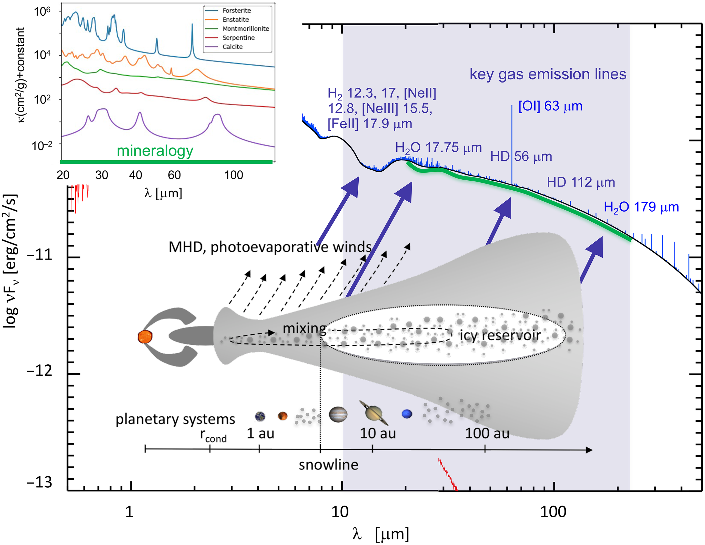
Figure 1. Sketch summarising where SPICA provides unique insight into how planetary systems form.
2. Disk gas masses
Over the past three decades, many different observational techniques have been employed to measure disk masses (roughly ordered in time): mm-continuum fluxes, CO line fluxes, mm-continuum and sub-mm line interferometry, CO isotopologue line ratios, [O I]
 $63\,\mu\mathrm{m}$
+ CO sub-mm lines, HD line(s), and wavelength-dependent dust outer radii. Important steps in the disk mass determination were (1) the use of disk models in the interpretation of interferometric data, (2) the recent revision of dust opacities, and (3) the combined interpretation of multi-wavelength datasets. We discuss below the most recently employed techniques to estimate disk masses as well as the advantages and disadvantages of each method.
$63\,\mu\mathrm{m}$
+ CO sub-mm lines, HD line(s), and wavelength-dependent dust outer radii. Important steps in the disk mass determination were (1) the use of disk models in the interpretation of interferometric data, (2) the recent revision of dust opacities, and (3) the combined interpretation of multi-wavelength datasets. We discuss below the most recently employed techniques to estimate disk masses as well as the advantages and disadvantages of each method.
Continuum mm/sub-mm fluxes: Thermal continuum emission can be used to determine the dust mass within a disk under the assumption of a dust opacity (typically uncertain by at least a factor of 2) and a dust temperature (better modelled as varying with radial location in the disk). Reliable estimates of the dust mass also require attention to the optical depth (Beckwith et al. Reference Beckwith, Sargent, Chini and Guesten1990). Recent ALMA observations raise again the possibility that the inner parts of planet-forming disks are optically thick (Ballering & Eisner Reference Ballering and Eisner2019; Zhu et al. Reference Zhu2019). Woitke et al. (Reference Woitke2016) show how the assumptions of a single-representative dust temperature and an optically thick contribution to the emission affect the dust mass derivation. Once the dust mass is determined, conversion to gas mass requires an estimate of the dust to gas ratio which is usually assumed to be 100 (based on the canonical interstellar medium value).
CO sub-mm and [O I]
 $\boldsymbol{63\,\mu}\textbf{m}$
: Herschel was able to detect the strongest gas cooling line from planet-forming disks, the [O I]
$\boldsymbol{63\,\mu}\textbf{m}$
: Herschel was able to detect the strongest gas cooling line from planet-forming disks, the [O I]
 $63\,\mu\mathrm{m}$
line, in a large fraction of young planet-forming disks (Dent et al. Reference Dent2013; Riviere-Marichalar et al. Reference Riviere-Marichalar, Merín, Kamp, Eiroa and Montesinos2016). The [O I] 63-
$63\,\mu\mathrm{m}$
line, in a large fraction of young planet-forming disks (Dent et al. Reference Dent2013; Riviere-Marichalar et al. Reference Riviere-Marichalar, Merín, Kamp, Eiroa and Montesinos2016). The [O I] 63-
 $\mu\mathrm{m}$
line-emitting region shifts, radially and vertically, with disk mass, making it an indirect tracer in combination with a temperature indicator. Hence, in combination with a CO sub-mm line, these fine structure line fluxes can be used to estimate disk masses within a factor of 3 (Kamp et al. Reference Kamp, Woitke, Pinte, Tilling, Thi, Menard, Duchene and Augereau2011; Meeus et al. Reference Meeus2012). However, for disks with gas masses above
$\mu\mathrm{m}$
line-emitting region shifts, radially and vertically, with disk mass, making it an indirect tracer in combination with a temperature indicator. Hence, in combination with a CO sub-mm line, these fine structure line fluxes can be used to estimate disk masses within a factor of 3 (Kamp et al. Reference Kamp, Woitke, Pinte, Tilling, Thi, Menard, Duchene and Augereau2011; Meeus et al. Reference Meeus2012). However, for disks with gas masses above
 $\sim\!10^{-3}\,\mathrm{M}_\odot$
, or for disks with non-solar carbon and/or oxygen abundances, this method becomes highly uncertain.
$\sim\!10^{-3}\,\mathrm{M}_\odot$
, or for disks with non-solar carbon and/or oxygen abundances, this method becomes highly uncertain.
CO isotopologue sub-mm lines: A more direct estimate of disk gas mass comes from the observations of the rotational lines of CO and its rarer isotopologuesFootnote a (
 $^{13}\mathrm{CO}$
,
$^{13}\mathrm{CO}$
,
 $\mathrm{C}^{18}\mathrm{O}$
,
$\mathrm{C}^{18}\mathrm{O}$
,
 $^{13}\mathrm{C}^{18}\mathrm{O}$
, and
$^{13}\mathrm{C}^{18}\mathrm{O}$
, and
 $^{13}\mathrm{C}^{17}\mathrm{O}$
) using (sub)-millimetre telescopes. The rarer isotopologues are optically thinner and hence trace disk regions down to the CO iceline. The uncertainty in the gas-phase abundances of these species relative to
$^{13}\mathrm{C}^{17}\mathrm{O}$
) using (sub)-millimetre telescopes. The rarer isotopologues are optically thinner and hence trace disk regions down to the CO iceline. The uncertainty in the gas-phase abundances of these species relative to
 $\mathrm{H}_2$
molecules, however, limits the measurement reliability. In addition, CO rotational lines predominantly measure the cold gas mass, typically residing beyond 50 au. Processes such as CO freeze-out (Panić & Hogerheijde Reference Panić and Hogerheijde2009) and CO isotope selective photodissociation, by stellar and interstellar photons (Miotello, Bruderer, & van Dishoeck Reference Miotello, Bruderer and van Dishoeck2014; Reference Miotello, van Dishoeck, Kama and Bruderer2016), as well as the gas phase carbon and oxygen abundances (Bruderer et al. Reference Bruderer, van Dishoeck, Doty and Herczeg2012; Miotello et al. Reference Miotello2017) affect these gas mass estimates. Williams & Best (Reference Williams and Best2014) consider use of the fluxes of the two rarer isotopologues
$\mathrm{H}_2$
molecules, however, limits the measurement reliability. In addition, CO rotational lines predominantly measure the cold gas mass, typically residing beyond 50 au. Processes such as CO freeze-out (Panić & Hogerheijde Reference Panić and Hogerheijde2009) and CO isotope selective photodissociation, by stellar and interstellar photons (Miotello, Bruderer, & van Dishoeck Reference Miotello, Bruderer and van Dishoeck2014; Reference Miotello, van Dishoeck, Kama and Bruderer2016), as well as the gas phase carbon and oxygen abundances (Bruderer et al. Reference Bruderer, van Dishoeck, Doty and Herczeg2012; Miotello et al. Reference Miotello2017) affect these gas mass estimates. Williams & Best (Reference Williams and Best2014) consider use of the fluxes of the two rarer isotopologues
 $^{13}\mathrm{CO}$
and
$^{13}\mathrm{CO}$
and
 $\mathrm{C}^{18}\mathrm{O}$
to derive disk gas mass estimates. The method was refined by Miotello et al. (Reference Miotello, van Dishoeck, Kama and Bruderer2016), accounting self-consistently for isotope selective dissociation. Both grids of models, however, neglect the gas-to-dust mass ratio as a confounding parameter in their study; Woitke et al. (Reference Woitke2016) show that the gas-to-dust parameter can strongly affect the CO isotopologue line fluxes; the local gas-to-dust mass ratio determines the disk temperature and affects the location of the CO iceline as well as the gas temperature of the emitting CO isotopologues. Thus, we require an iterative approach, relying on successive dust and the gas mass determinations. And again, chemical effects changing the canonical CO-to-
$\mathrm{C}^{18}\mathrm{O}$
to derive disk gas mass estimates. The method was refined by Miotello et al. (Reference Miotello, van Dishoeck, Kama and Bruderer2016), accounting self-consistently for isotope selective dissociation. Both grids of models, however, neglect the gas-to-dust mass ratio as a confounding parameter in their study; Woitke et al. (Reference Woitke2016) show that the gas-to-dust parameter can strongly affect the CO isotopologue line fluxes; the local gas-to-dust mass ratio determines the disk temperature and affects the location of the CO iceline as well as the gas temperature of the emitting CO isotopologues. Thus, we require an iterative approach, relying on successive dust and the gas mass determinations. And again, chemical effects changing the canonical CO-to-
 $\mathrm{H}_2$
conversion factor continue to present a significant source of uncertainty (Yu et al. Reference Yu, Evans Neal, Dodson-Robinson, Willacy and Turner2017; Molyarova et al. Reference Molyarova, Akimkin, Semenov, Henning, Vasyunin and Wiebe2017).
$\mathrm{H}_2$
conversion factor continue to present a significant source of uncertainty (Yu et al. Reference Yu, Evans Neal, Dodson-Robinson, Willacy and Turner2017; Molyarova et al. Reference Molyarova, Akimkin, Semenov, Henning, Vasyunin and Wiebe2017).
HD: The major constituent of the disk gas is molecular hydrogen,
 $\mathrm{H}_2$
, but its rotational lines are not sensitive to main disk temperature conditions, that is, these lines are not effective disk mass tracers. The deuterated variant, HD, has a very simple chemistry and is expected to have a constant abundance of
$\mathrm{H}_2$
, but its rotational lines are not sensitive to main disk temperature conditions, that is, these lines are not effective disk mass tracers. The deuterated variant, HD, has a very simple chemistry and is expected to have a constant abundance of
 $2 \pm 0.1 \times 10^{-5}$
(the average local ISM value, Prodanović et al. Reference Prodanović, Steigman and Fields2010) throughout the disk. This constancy makes the lowest two HD rotational lines—
$2 \pm 0.1 \times 10^{-5}$
(the average local ISM value, Prodanović et al. Reference Prodanović, Steigman and Fields2010) throughout the disk. This constancy makes the lowest two HD rotational lines—
 $J=1{-}0$
at
$J=1{-}0$
at
 $112\,\mu\mathrm{m}$
(
$112\,\mu\mathrm{m}$
(
 $E_{\rm up}=128.5\,\mathrm{K}$
) and HD
$E_{\rm up}=128.5\,\mathrm{K}$
) and HD
 $J=2{-}1$
at 56
$J=2{-}1$
at 56
 $\mu\mathrm{m}$
(
$\mu\mathrm{m}$
(
 $E_{\rm up}=384.6\,\mathrm{K}$
)—reliable tracers of the warm gas mass in the inner disk (inside
$E_{\rm up}=384.6\,\mathrm{K}$
)—reliable tracers of the warm gas mass in the inner disk (inside
 $\sim\!100\,\mathrm{au}$
). These inner disk regions are of prime importance since the majority of planets are thought to be formed there, rather than in the cold outer disk beyond
$\sim\!100\,\mathrm{au}$
). These inner disk regions are of prime importance since the majority of planets are thought to be formed there, rather than in the cold outer disk beyond
 $\sim\!100\,\mathrm{au}$
where CO sub-mm lines become good tracers of mass. Bergin et al. (Reference Bergin2013) and McClure et al. (Reference McClure2016) detected the lower excitation HD line in three planet-forming disks with Herschel/PACS and Kama et al. (Reference Kama2020) derived upper limits to the gas masses for disks around 15 objects from Herschel upper limits on both HD lines.
$\sim\!100\,\mathrm{au}$
where CO sub-mm lines become good tracers of mass. Bergin et al. (Reference Bergin2013) and McClure et al. (Reference McClure2016) detected the lower excitation HD line in three planet-forming disks with Herschel/PACS and Kama et al. (Reference Kama2020) derived upper limits to the gas masses for disks around 15 objects from Herschel upper limits on both HD lines.
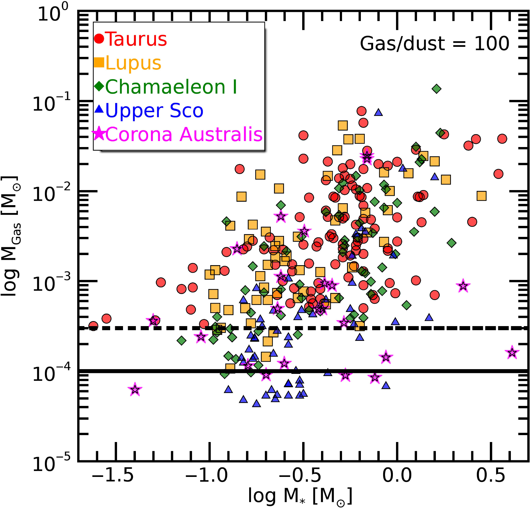
Figure 2. Distribution of disk masses as a function of the stellar mass for nearby star-forming regions, based on recent millimetre dust continuum observations with the SMA and ALMA (Andrews et al. Reference Andrews, Rosenfeld, Kraus and Wilner2013; Ansdell et al. Reference Ansdell2016; Barenfeld et al. Reference Barenfeld, Carpenter, Ricci and Isella2016; Pascucci et al. Reference Pascucci2016; Cieza et al. Reference Cieza2019; Cazzoletti et al. Reference Cazzoletti2019) and assuming a global gas-to-dust mass ratio of 100. The two horizontal lines indicate the detection limits that will be achieved with SAFARI observations of the HD
 $J=1{-}0$
line fluxes in the case of the shallow (1 h on-source, dashed line) and deep (10 h on-source, dotted) surveys, following the HD line flux predictions from Trapman et al. (Reference Trapman, Miotello, Kama, van Dishoeck and Bruderer2017).
$J=1{-}0$
line fluxes in the case of the shallow (1 h on-source, dashed line) and deep (10 h on-source, dotted) surveys, following the HD line flux predictions from Trapman et al. (Reference Trapman, Miotello, Kama, van Dishoeck and Bruderer2017).
2.1. Disk gas masses from HD lines with SPICA
Over the next decade, we anticipate ALMA to have undertaken complete disk surveys (dust and CO isotopologues) in all relevant nearby star-forming regions (within
 $500\,\mathrm{pc}$
). For large,
$500\,\mathrm{pc}$
). For large,
 $>\!100\,\mathrm{au}$
, disks in low-mass star-forming regions, most of the disk gas mass is expected to be well below 50 K; with ALMA, we will thus have a good understanding of the cold outer disk component. Planet formation similar to our Solar System, however, happens in the inner regions of the disk, inside 100 au, and Trapman et al. (Reference Trapman, Miotello, Kama, van Dishoeck and Bruderer2017) showed that most of the HD emission is originating along the inner warm disk surfaces (
$>\!100\,\mathrm{au}$
, disks in low-mass star-forming regions, most of the disk gas mass is expected to be well below 50 K; with ALMA, we will thus have a good understanding of the cold outer disk component. Planet formation similar to our Solar System, however, happens in the inner regions of the disk, inside 100 au, and Trapman et al. (Reference Trapman, Miotello, Kama, van Dishoeck and Bruderer2017) showed that most of the HD emission is originating along the inner warm disk surfaces (
 $50{-}200\,\mathrm{K}$
). Furthermore, ALMA surveys have shown recently that the majority of disks are likely smaller than 100 au (Ansdell et al. Reference Ansdell2018; Long et al. Reference Long2019), making HD a direct tracer of the bulk gas mass for those objects. On the other hand, in high-mass star-forming regions, the external radiation field of nearby O/B stars could warm the entire disk surface well above 50 K, enhancing the importance of HD measurements.
$50{-}200\,\mathrm{K}$
). Furthermore, ALMA surveys have shown recently that the majority of disks are likely smaller than 100 au (Ansdell et al. Reference Ansdell2018; Long et al. Reference Long2019), making HD a direct tracer of the bulk gas mass for those objects. On the other hand, in high-mass star-forming regions, the external radiation field of nearby O/B stars could warm the entire disk surface well above 50 K, enhancing the importance of HD measurements.
Both HD lines (
 $J=1{-}0$
and
$J=1{-}0$
and
 $J=2{-}1$
at 112 and
$J=2{-}1$
at 112 and
 $56\,\mu\mathrm{m}$
, respectively) are only accessible from space/stratosphere and SAFARI is uniquely equipped in terms of spectral coverage and sensitivity to measure them across statistical samples of disks. For an observational estimate of the gas mass in the planet-forming region, within 100 au, the HD line ratio will be a proxy of the ‘disk gas temperature’ and the line fluxes will be used to derive disk mass estimates using model grids, similar to what has been done with ALMA for the CO isotopologues (Miotello et al. Reference Miotello2017; Long et al. Reference Long2018). These model grids can be easily refined, taking the disk substructure known from the ALMA surveys into account. Since the HD abundance is not affected by element abundances/chemistry/freeze-out, this remains the most robust technique to estimate disk gas masses.
$56\,\mu\mathrm{m}$
, respectively) are only accessible from space/stratosphere and SAFARI is uniquely equipped in terms of spectral coverage and sensitivity to measure them across statistical samples of disks. For an observational estimate of the gas mass in the planet-forming region, within 100 au, the HD line ratio will be a proxy of the ‘disk gas temperature’ and the line fluxes will be used to derive disk mass estimates using model grids, similar to what has been done with ALMA for the CO isotopologues (Miotello et al. Reference Miotello2017; Long et al. Reference Long2018). These model grids can be easily refined, taking the disk substructure known from the ALMA surveys into account. Since the HD abundance is not affected by element abundances/chemistry/freeze-out, this remains the most robust technique to estimate disk gas masses.
Figure 2 shows the ALMA disk samples for which dust masses have been measured in five star-forming regions (Taurus, Lupus, Chameleon I, Upper Sco, and Corona Australis, from Andrews et al. Reference Andrews, Rosenfeld, Kraus and Wilner2013; Ansdell et al. Reference Ansdell2016; Barenfeld et al. Reference Barenfeld, Carpenter, Ricci and Isella2016; Pascucci et al. Reference Pascucci2016; Cieza et al. Reference Cieza2019; Cazzoletti et al. Reference Cazzoletti2019). We assume here a gas-to-dust mass ratio of 100 and indicate the SAFARI sensitivity limits based on a 1 and 10 h per source deep survey. If all the disks in these surveys are T Tauri disks with disk/stellar properties similar to those modelled by Trapman et al. (Reference Trapman, Miotello, Kama, van Dishoeck and Bruderer2017), the HD line flux predictions reveal that we can detect the gaseous counterpart from all ALMA dust-detected disks. Both HD lines are optically thin for disks as massive as a few
 $10^{-2}\,M_{\odot}$
(i.e., a few times the value of the minimum mass Solar Nebula, Trapman et al. Reference Trapman, Miotello, Kama, van Dishoeck and Bruderer2017). The vast majority of the ALMA-surveyed disk population has a total gas mass below this limit, utilising a gas-to-dust ratio of 100. Therefore, HD line flux measurements, together with the constant HD abundance, provide a temperature and gas column density estimate which can be converted into a precise mass estimate of the gas. Figure 3 demonstrates the feasibility of this approach across a grid of T Tauri disk models (Trapman et al. Reference Trapman, Miotello, Kama, van Dishoeck and Bruderer2017). Combined with ALMA dust continuum fluxes, the SAFARI measurements of the two HD lines will provide the most complete survey for bulk gas mass estimates and gas-to-dust mass ratios for disk planet-forming regions at a sensitivity comparable to that of the current ALMA dust surveys (Ansdell et al. Reference Ansdell2016; Barenfeld et al. Reference Barenfeld, Carpenter, Ricci and Isella2016; Pascucci et al. Reference Pascucci2016; Long et al. Reference Long2018; Cieza et al. Reference Cieza2019; Cazzoletti et al. Reference Cazzoletti2019). Having HD gas masses for statistically relevant disk samples allows also to calibrate and understand the issues around the CO isotopologue mass estimate.
$10^{-2}\,M_{\odot}$
(i.e., a few times the value of the minimum mass Solar Nebula, Trapman et al. Reference Trapman, Miotello, Kama, van Dishoeck and Bruderer2017). The vast majority of the ALMA-surveyed disk population has a total gas mass below this limit, utilising a gas-to-dust ratio of 100. Therefore, HD line flux measurements, together with the constant HD abundance, provide a temperature and gas column density estimate which can be converted into a precise mass estimate of the gas. Figure 3 demonstrates the feasibility of this approach across a grid of T Tauri disk models (Trapman et al. Reference Trapman, Miotello, Kama, van Dishoeck and Bruderer2017). Combined with ALMA dust continuum fluxes, the SAFARI measurements of the two HD lines will provide the most complete survey for bulk gas mass estimates and gas-to-dust mass ratios for disk planet-forming regions at a sensitivity comparable to that of the current ALMA dust surveys (Ansdell et al. Reference Ansdell2016; Barenfeld et al. Reference Barenfeld, Carpenter, Ricci and Isella2016; Pascucci et al. Reference Pascucci2016; Long et al. Reference Long2018; Cieza et al. Reference Cieza2019; Cazzoletti et al. Reference Cazzoletti2019). Having HD gas masses for statistically relevant disk samples allows also to calibrate and understand the issues around the CO isotopologue mass estimate.
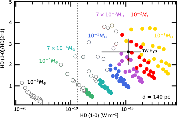
Figure 3. HD diagnostic diagram: Disk gas masses can be derived from a combination of the two HD lines, based on a grid of T Tauri disk models from Trapman et al. (Reference Trapman, Miotello, Kama, van Dishoeck and Bruderer2017). Open symbols denote disk model predictions for a distance of 140 pc (e.g., the Taurus star-forming region), where SPICA will not be able to detect both HD lines in a SAFARI/HR 1 h integration
 $(\!<\!5\,\sigma$
) due to the lower sensitivity at
$(\!<\!5\,\sigma$
) due to the lower sensitivity at
 $56\,\mu\mathrm{m}$
(the higher continuum lowers the line sensitivity). The black dot with error bars shows the only object, TW Hya (
$56\,\mu\mathrm{m}$
(the higher continuum lowers the line sensitivity). The black dot with error bars shows the only object, TW Hya (
 $60.1\,\mathrm{pc}$
, put here at a distance of 140 pc), for which both HD lines have been measured with Herschel/PACS. The vertical dotted line indicates the 1 h sensitivity limit (
$60.1\,\mathrm{pc}$
, put here at a distance of 140 pc), for which both HD lines have been measured with Herschel/PACS. The vertical dotted line indicates the 1 h sensitivity limit (
 $5\,\sigma$
) for the HD
$5\,\sigma$
) for the HD
 $J=1{-}0$
line.
$J=1{-}0$
line.
To mitigate the temperature dependence of the HD gas mass estimates, we will use the
 $^{12}\mathrm{CO}$
and
$^{12}\mathrm{CO}$
and
 $^{13}\mathrm{CO}$
rotational ladders to derive the 2D temperature structure (see Section 2.2), providing an improvement over the simple HD line ratio ‘disk gas temperature’ estimate. We will thus measure the total gas mass from a simultaneous fit of the two HD line fluxes and the
$^{13}\mathrm{CO}$
rotational ladders to derive the 2D temperature structure (see Section 2.2), providing an improvement over the simple HD line ratio ‘disk gas temperature’ estimate. We will thus measure the total gas mass from a simultaneous fit of the two HD line fluxes and the
 $^{12}\mathrm{CO}$
and
$^{12}\mathrm{CO}$
and
 $^{13}\mathrm{CO}$
rotational ladders (e.g., Fedele et al. Reference Fedele, van Dishoeck, Kama, Bruderer and Hogerheijde2016).
$^{13}\mathrm{CO}$
rotational ladders (e.g., Fedele et al. Reference Fedele, van Dishoeck, Kama, Bruderer and Hogerheijde2016).
Disk flaring is key for the gas heating and disk temperature structure (Kamp et al. Reference Kamp, Woitke, Pinte, Tilling, Thi, Menard, Duchene and Augereau2011, e.g.). Hence, to further refine the disk gas mass estimates, the [O I] fine structure lines have been shown to be sensitive tracers of disk flaring out to
 $\sim\!100\,\mathrm{au}$
(regions where HD is also predicted to emit, Reference Trapman, Miotello, Kama, van Dishoeck and BrudererTrapman et al. 2017) and good probes of disk gas temperature (Woitke et al. Reference Woitke, Pinte, Tilling, Ménard, Kamp, Thi, Duchêne and Augereau2010; Kamp et al. Reference Kamp, Woitke, Pinte, Tilling, Thi, Menard, Duchene and Augereau2011); the [O I]
$\sim\!100\,\mathrm{au}$
(regions where HD is also predicted to emit, Reference Trapman, Miotello, Kama, van Dishoeck and BrudererTrapman et al. 2017) and good probes of disk gas temperature (Woitke et al. Reference Woitke, Pinte, Tilling, Ménard, Kamp, Thi, Duchêne and Augereau2010; Kamp et al. Reference Kamp, Woitke, Pinte, Tilling, Thi, Menard, Duchene and Augereau2011); the [O I]
 $63\,\mu\mathrm{m}$
line is the brightest cooling line in disks, regularly detected with Herschel, and hence will be detected routinely with SPICA.
$63\,\mu\mathrm{m}$
line is the brightest cooling line in disks, regularly detected with Herschel, and hence will be detected routinely with SPICA.
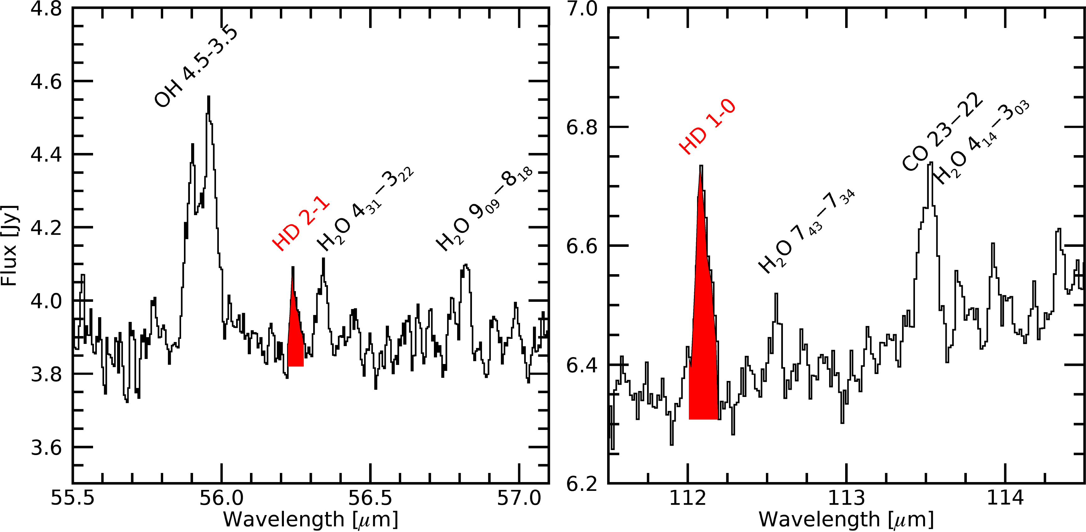
Figure 4. Herschel/PACS spectrum of TW Hya showing the detection of the lowest two HD rotational lines at
 $56\,\mu\mathrm{m}$
and
$56\,\mu\mathrm{m}$
and
 $112\,\mu\mathrm{m}$
(spectra re-reduced by D. Fedele).
$112\,\mu\mathrm{m}$
(spectra re-reduced by D. Fedele).
ALMA CO surveys can provide radial surface gas density profiles. The combination of ALMA CO and far-IR [O i] together with modelling lines can break degeneracies in the determination of disk masses. Ancillary and routine detection of the [O I]
 ${63, 145}\,\mu\textrm{m}$
and [C II]
${63, 145}\,\mu\textrm{m}$
and [C II]
 ${158}\,\mu\textrm{m}$
lines with SAFARI, can also address the frequently discussed question of the disk C/O abundances being different from typical ISM values, possibly due to planet-forming processes, migration of icy planetesimals, and filtering of sizes due to dust traps (see e.g., Cleeves et al. Reference Cleeves, Öberg, Wilner, Huang, Loomis, Andrews and Guzman2018; Miotello et al. Reference Miotello2019).
${158}\,\mu\textrm{m}$
lines with SAFARI, can also address the frequently discussed question of the disk C/O abundances being different from typical ISM values, possibly due to planet-forming processes, migration of icy planetesimals, and filtering of sizes due to dust traps (see e.g., Cleeves et al. Reference Cleeves, Öberg, Wilner, Huang, Loomis, Andrews and Guzman2018; Miotello et al. Reference Miotello2019).
The HD lines do not need to be spectrally resolved in the SAFARI wavelength range. However, since molecular lines have a very low line-to-continuum ratio
 $({\lesssim}0.05$
), that is, weak narrow gas lines (unresolved) on a strong continuum, we require a spectral resolution of at least a few 1 000 to maximise the line detection rate (see Trapman et al. Reference Trapman, Miotello, Kama, van Dishoeck and Bruderer2017, for a detailed discussion). The low excitation HD lines,
$({\lesssim}0.05$
), that is, weak narrow gas lines (unresolved) on a strong continuum, we require a spectral resolution of at least a few 1 000 to maximise the line detection rate (see Trapman et al. Reference Trapman, Miotello, Kama, van Dishoeck and Bruderer2017, for a detailed discussion). The low excitation HD lines,
 $J=1{-}0$
,
$J=1{-}0$
,
 $J=2{-}1$
, are expected to have typical widths of
$J=2{-}1$
, are expected to have typical widths of
 $5{-}20\ \mathrm{km\ s}^{-1}$
, dependent also on inclination. Figure 4 shows that even with the Herschel/PACS resolution of
$5{-}20\ \mathrm{km\ s}^{-1}$
, dependent also on inclination. Figure 4 shows that even with the Herschel/PACS resolution of
 $R \sim 1500$
, the HD lines were not blended. Given the higher spectral resolution of SAFARI/Fourier Tranform Spectrometer (FTS) (
$R \sim 1500$
, the HD lines were not blended. Given the higher spectral resolution of SAFARI/Fourier Tranform Spectrometer (FTS) (
 $R \sim 7\,300$
and
$R \sim 7\,300$
and
 $3\,700$
at 56 and 112
$3\,700$
at 56 and 112
 $\mu\mathrm{m}$
respectively) line fluxes can be extracted in a straightforward manner.
$\mu\mathrm{m}$
respectively) line fluxes can be extracted in a straightforward manner.
From thermo-chemical disk models by Trapman et al. (Reference Trapman, Miotello, Kama, van Dishoeck and Bruderer2017) for T Tauri disks spanning a typical range of disk properties (flaring, disk size, and scale heights), we find HD
 $J=1{-}0$
line fluxes ranging from
$J=1{-}0$
line fluxes ranging from
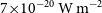 $7\!\times\!10^{-20}\,\mathrm{W\,m}^{-2}$
for
$7\!\times\!10^{-20}\,\mathrm{W\,m}^{-2}$
for
 $10^{-4}\,\mathrm{M}_\odot$
disks (low mass, optically thin) to
$10^{-4}\,\mathrm{M}_\odot$
disks (low mass, optically thin) to
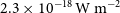 $2.3 \times 10^{-18}\,\mathrm{W\,m}^{-2}$
for
$2.3 \times 10^{-18}\,\mathrm{W\,m}^{-2}$
for
 $10^{-1}\,\mathrm{M}_\odot$
disks (massive, optically thick). The HD
$10^{-1}\,\mathrm{M}_\odot$
disks (massive, optically thick). The HD
 $J=2{-}1$
line is stronger for low-mass optically thin disks (
$J=2{-}1$
line is stronger for low-mass optically thin disks (
 $10^{-19}\,\mathrm{W\,m}^{-2}$
) and fainter for optically thick massive disks (
$10^{-19}\,\mathrm{W\,m}^{-2}$
) and fainter for optically thick massive disks (
 $10^{-18}\,\mathrm{W\,m}^{-2}$
).
$10^{-18}\,\mathrm{W\,m}^{-2}$
).
Since the line fluxes scale with the continuum (see Figure 19 in Appendix A.1), we propose a survey based on the continuum brightness of the sources. The HD
 $J=1{-}0$
and
$J=1{-}0$
and
 $J=2{-}1$
lines fall into the long (LW) and medium wavelength band (MW) with a spectral resolution of
$J=2{-}1$
lines fall into the long (LW) and medium wavelength band (MW) with a spectral resolution of
 $R \sim 3\,700$
and
$R \sim 3\,700$
and
 $R \sim 7\,300$
, respectively. For sources with a continuum flux
$R \sim 7\,300$
, respectively. For sources with a continuum flux
 $<\!0.1\,\mathrm{Jy}$
(MW) and
$<\!0.1\,\mathrm{Jy}$
(MW) and
 $<\!1\,\mathrm{Jy}$
(LW), respectively, SAFARI/HR reaches a line sensitivity of
$<\!1\,\mathrm{Jy}$
(LW), respectively, SAFARI/HR reaches a line sensitivity of
 $\sim\!1.3 \times 10^{-19}\,\mathrm{W\,m}^{-2}$
in 1 h (
$\sim\!1.3 \times 10^{-19}\,\mathrm{W\,m}^{-2}$
in 1 h (
 $5\,\sigma$
); this corresponds to disk gas masses down to
$5\,\sigma$
); this corresponds to disk gas masses down to
 $\sim\!10^{-3}\,\mathrm{M}_\odot$
. We will set our integration times in the HD disk gas mass survey such that we can push down to
$\sim\!10^{-3}\,\mathrm{M}_\odot$
. We will set our integration times in the HD disk gas mass survey such that we can push down to
 $2 \times 10^{-4}\,\mathrm{M}_\odot$
while still detecting both HD lines. Figure 2 shows that we would be able to provide, in a survey with
$2 \times 10^{-4}\,\mathrm{M}_\odot$
while still detecting both HD lines. Figure 2 shows that we would be able to provide, in a survey with
 $1{-}10$
h integration times, reliable gas mass estimates for all disks that are currently detected in dust surveys of star-forming regions with ALMA. The sensitivity limit also overlaps with the upper end of the gas masses detected via CO in debris disks (Moór et al. Reference Moór2019, see Section 4). Should those disks harbour remnant primordial gas from the younger phase (instead of secondary
$1{-}10$
h integration times, reliable gas mass estimates for all disks that are currently detected in dust surveys of star-forming regions with ALMA. The sensitivity limit also overlaps with the upper end of the gas masses detected via CO in debris disks (Moór et al. Reference Moór2019, see Section 4). Should those disks harbour remnant primordial gas from the younger phase (instead of secondary
 $\mathrm{H}_2$
-poor gas), we would detect that gas in the HD lines. Including in the survey a statistically significant number of class III disks, potentially young debris disks, we will be able to determine for the first time the transition from primordial to secondary gas.
$\mathrm{H}_2$
-poor gas), we would detect that gas in the HD lines. Including in the survey a statistically significant number of class III disks, potentially young debris disks, we will be able to determine for the first time the transition from primordial to secondary gas.
2.2. Radial temperature profiles—The co-ladder
Disks are not isothermal structures. Rather, they are characterised by a large gradient in the gas temperature, which can go from nearly
 $10^3\,\mathrm{K}$
in the proximity of the star down to
$10^3\,\mathrm{K}$
in the proximity of the star down to
 $\sim\!10\,\mathrm{K}$
(or even lower) in the outer part of the disk midplane. Knowledge of the gas temperature gradient is important for the interpretation of both molecular and atomic spectra, as
$\sim\!10\,\mathrm{K}$
(or even lower) in the outer part of the disk midplane. Knowledge of the gas temperature gradient is important for the interpretation of both molecular and atomic spectra, as
 $T_{\rm gas}$
regulates line intensities. The vertical gas temperature gradient is, for example, key to understanding the emission from CO isotopologues which probe successively deeper layers in the disk (Dartois et al. Reference Dartois, Dutrey and Guilloteau2003). Moreover, the local gas temperature also controls the gas chemistry, hence the formation of molecules and the resultant chemical enrichment. For example, at warm temperatures (
$T_{\rm gas}$
regulates line intensities. The vertical gas temperature gradient is, for example, key to understanding the emission from CO isotopologues which probe successively deeper layers in the disk (Dartois et al. Reference Dartois, Dutrey and Guilloteau2003). Moreover, the local gas temperature also controls the gas chemistry, hence the formation of molecules and the resultant chemical enrichment. For example, at warm temperatures (
 $>\!200\,\mathrm{K}$
), neutral-neutral chemistry can proceed to efficiently form water via the radiative association H + OH (Glassgold et al. Reference Glassgold, Meijerink and Najita2009; Kamp et al. Reference Kamp2013).
$>\!200\,\mathrm{K}$
), neutral-neutral chemistry can proceed to efficiently form water via the radiative association H + OH (Glassgold et al. Reference Glassgold, Meijerink and Najita2009; Kamp et al. Reference Kamp2013).
An ideal thermometer of disk surface layers is the CO rotational ladder: the CO rotational transitions are optically thick and, due to their low critical density, are quickly thermalised in disks. Moreover, the CO transitions span a large range of upper energy levels, from 5.5 K (
 $J=1{-}0$
) up to a few 1 000 K (for
$J=1{-}0$
) up to a few 1 000 K (for
 $J_{\rm up} > 20$
), see Table 1. Rotational lines up to
$J_{\rm up} > 20$
), see Table 1. Rotational lines up to
 $J=10{-}9$
can be obtained from the ground, but the higher rotational lines are uniquely measured from space. As such the CO rotational ladder provides direct information about the kinetic temperature throughout the entire disk surface. In particular, a simultaneous model fit to the various CO transitions allows us to constrain the 2D temperature structure, not only the radial gradient but also the vertical gradient in the surface. Additional constraints to the vertical gradient reaching deeper into the disk are provided by the
$J=10{-}9$
can be obtained from the ground, but the higher rotational lines are uniquely measured from space. As such the CO rotational ladder provides direct information about the kinetic temperature throughout the entire disk surface. In particular, a simultaneous model fit to the various CO transitions allows us to constrain the 2D temperature structure, not only the radial gradient but also the vertical gradient in the surface. Additional constraints to the vertical gradient reaching deeper into the disk are provided by the
 $^{13}\mathrm{CO}$
ladder. Due to the lower optical depth with respect to the main isotopologue, the
$^{13}\mathrm{CO}$
ladder. Due to the lower optical depth with respect to the main isotopologue, the
 $^{13}\mathrm{CO}$
transitions probe different density and temperature regions inside the disk. Figure 5 shows that we can routinely detect the CO ladder in our HD survey (
$^{13}\mathrm{CO}$
transitions probe different density and temperature regions inside the disk. Figure 5 shows that we can routinely detect the CO ladder in our HD survey (
 $1{-}10\,\mathrm{h}$
exposure times) toward the warm disks around Herbig stars, and typically up to
$1{-}10\,\mathrm{h}$
exposure times) toward the warm disks around Herbig stars, and typically up to
 $J=17{-}16$
for the colder T Tauri disks.
$J=17{-}16$
for the colder T Tauri disks.
Table 1. Wavelengths and upper level energies (
 $E_{\rm up}$
) of CO lines to be observed with SAFARI to constrain the 2D gas temperature structure.
$E_{\rm up}$
) of CO lines to be observed with SAFARI to constrain the 2D gas temperature structure.
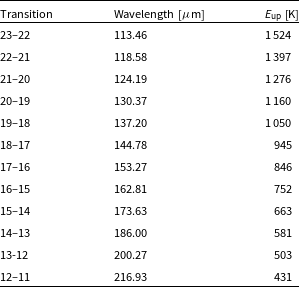
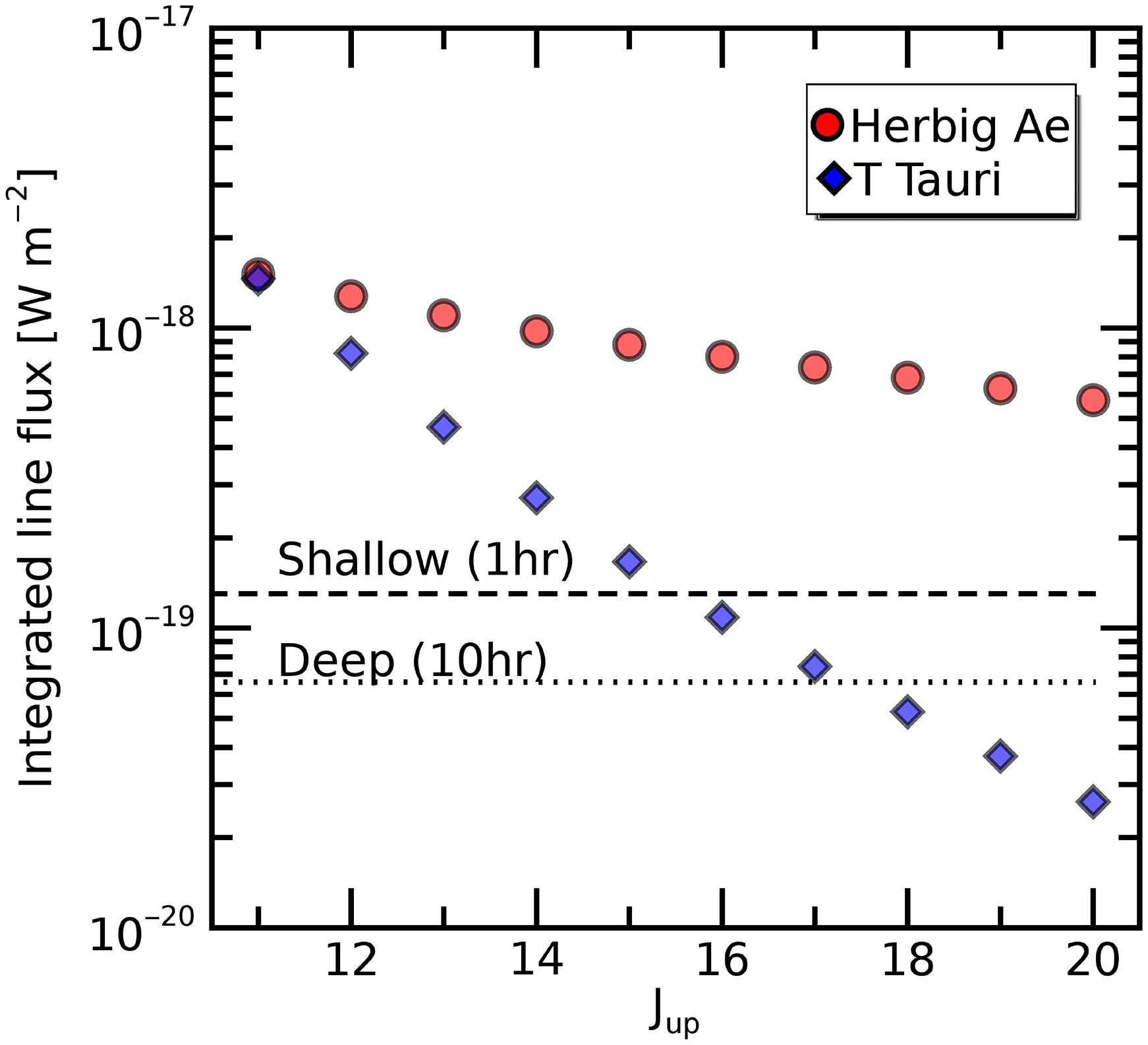
Figure 5. Predicted line flux of high-J CO rotational transitions in protoplanetary disks to be measured with SAFARI. The two models refer to the case of a flat disk with low scale height around a Herbig Ae star (spectral type A0,
 $20\,L_{\odot}$
) and to a cold T Tauri disk (K5,
$20\,L_{\odot}$
) and to a cold T Tauri disk (K5,
 $1.5\,L_{\odot}$
), both located at a distance of 140 pc from the Sun (DALI models, Reference Bruderer, van Dishoeck, Doty and Herczeg
Bruderer et al. 2012; Reference Bruderer
Bruderer 2013
). The two horizontal lines indicate the limiting line flux (
$1.5\,L_{\odot}$
), both located at a distance of 140 pc from the Sun (DALI models, Reference Bruderer, van Dishoeck, Doty and Herczeg
Bruderer et al. 2012; Reference Bruderer
Bruderer 2013
). The two horizontal lines indicate the limiting line flux (
 $5\,\sigma$
detection limit) for a shallow and deep survey, respectively.
$5\,\sigma$
detection limit) for a shallow and deep survey, respectively.
2.3. Disentangling disk and shock origin for HD
Often disks and shocks produce the same spectral lines in star-forming regions. In the absence of spatial resolution, spectral resolution can be used to disentangle these components. However, SPICA has only limited spectral resolution. We can overcome this by using diagnostic line ratios for disentangling disk and shocks. This is demonstrated in Figure 6, where we show the line ratio of CO (18-17)/CO (12–11) versus the line ratio of
 $\mathrm{H}_2\mathrm{O}\,4_{23}{-}3_{12}$
 $(78.74\,\mu\mathrm{m})/2_{12}{-}1_{01}(179.53\,\mu\mathrm{m}$
) for the disk models explored by the DENT (Disk Evolution with Neat Theory) grid (Woitke et al. Reference Woitke, Pinte, Tilling, Ménard, Kamp, Thi, Duchêne and Augereau2010; Kamp et al. Reference Kamp, Woitke, Pinte, Tilling, Thi, Menard, Duchene and Augereau2011) and for a non-dissociative shock models grid by Flower & Pineau des Forêts (Reference Flower and Pineau des Forêts2015). The figure shows that shocks and disks populate relatively separated areas of the line ratio plane. A larger contamination occurs only for dissociative shock models at the highest pre-shock density of
$(78.74\,\mu\mathrm{m})/2_{12}{-}1_{01}(179.53\,\mu\mathrm{m}$
) for the disk models explored by the DENT (Disk Evolution with Neat Theory) grid (Woitke et al. Reference Woitke, Pinte, Tilling, Ménard, Kamp, Thi, Duchêne and Augereau2010; Kamp et al. Reference Kamp, Woitke, Pinte, Tilling, Thi, Menard, Duchene and Augereau2011) and for a non-dissociative shock models grid by Flower & Pineau des Forêts (Reference Flower and Pineau des Forêts2015). The figure shows that shocks and disks populate relatively separated areas of the line ratio plane. A larger contamination occurs only for dissociative shock models at the highest pre-shock density of
 $10^4\,\mathrm{cm}^{-3}$
.
$10^4\,\mathrm{cm}^{-3}$
.
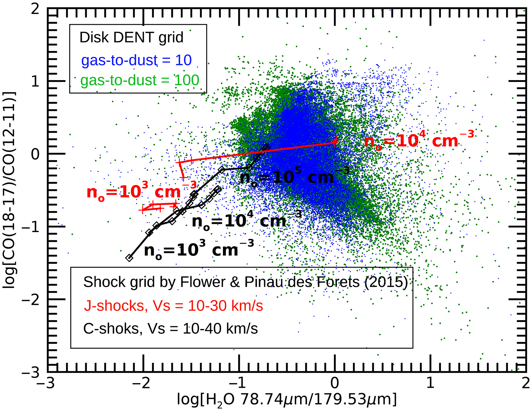
Figure 6. Line intensity ratio of CO(18-17)/CO(12-11) versus
 $\mathrm{H}_2\mathrm{O}\, 78\,\mu\mathrm{m}/179\,\mu\mathrm{m}$
line ratios predicted by the DENT grid of disk models compared with the predictions of J- and C-type shock models of Flower & Pineau des Forets (Reference Flower and Pineau des Forêts2015) for different pre-shock densities and pre-shock velocities.
$\mathrm{H}_2\mathrm{O}\, 78\,\mu\mathrm{m}/179\,\mu\mathrm{m}$
line ratios predicted by the DENT grid of disk models compared with the predictions of J- and C-type shock models of Flower & Pineau des Forets (Reference Flower and Pineau des Forêts2015) for different pre-shock densities and pre-shock velocities.
3. Disk dispersal—Setting the clock for planet formation
One important aspect of star and planet formation is the timescale for the dispersal of the protoplanetary disk. Indeed, it is crucial to determine how fast gas evaporates or gets accreted onto the central star, as the amount of gas available in the disk will set the clock for planet formation (see Alexander, McKeegan, and Altwegg Reference Alexander, Pascucci, Andrews, Armitage, Cieza, Beuther, Klessen, Dullemond and Henning2014). ALMA provides now increasing evidence that class ii disks may already host giant protoplanets (e.g., Reference AndrewsAndrews et al. 2018; Reference PintePinte et al. 2018). However, the gas dispersal timescale ends the runaway gas accretion onto giant protoplanets and halts their migration.
Broad-band near- to mid-IR excess (optically thick continuum emission from the dust) above the photospheric emission is an easy means to determine if an inner dust disk exists. The mean dispersal time is estimated from the fraction of such disks still observed as a function of the region’s age (e.g., Haisch Karl, Lada, & Lada Reference Helling, Woitke, Rimmer, Kamp, Thi and Meijerink2001; Hernández et al. Reference Hernández, Hartmann, Calvet, Jeffries, Gutermuth, Muzerolle and Stauffer2008; Mamajek Reference Mamajek, Usuda, Tamura and Ishii2009; Richert et al. Reference Richert, Getman, Feigelson, Kuhn, Broos, Povich, Bate and Garmire2018). Studies across many star-forming regions have allowed for the determination of a mean disk dispersal timescale of a few Myr; however, this method only traces the optically thick inner dust disk component, which comprises about 1% of the disk mass, and not the gas disk component, which drives the dynamics. Ohsawa et al. (Reference Ohsawa, Onaka and Yasui2015) showed that this method also leads to a bias in the estimate of the disk dissipation timescale if the disk mass function is not properly taken into account. Alternative studies using
 $\mathrm{H}\alpha$
emission, as a tracer for ongoing mass accretion and thus of the continued presence of gas in the disk, provide a similar, albeit possibly slightly shorter, timescale (Fedele et al. Reference Fedele, van den Ancker, Henning, Jayawardhana and Oliveira2010), suggesting a coevolving dust and gas disk with a somewhat longer-lived dust component. The few Myr timescale is comparable to the timescale expected for planet formation via the core accretion process, as well as to the timescale for giant planets to migrate (see Ercolano & Pascucci Reference Ercolano and Pascucci2017 for a detailed review). The exact mechanism of disk dispersal—photoevaporation and/or magneto-hydrodynamic (MHD) winds—and the amount of mass loss through these processes will therefore have important implications for gas giant planet formation, helping to constrain the available time for orbital migration or circularisation (Tanaka & Ward Reference Tanaka and Ward2004; Kikuchi et al. Reference Kikuchi, Higuchi and Ida2014). Inner disk evolution and dispersal, thus, play a crucial role in the final configuration of planetary systems, and there is a clear need for unbiased gas disk dispersal timescale studies.
$\mathrm{H}\alpha$
emission, as a tracer for ongoing mass accretion and thus of the continued presence of gas in the disk, provide a similar, albeit possibly slightly shorter, timescale (Fedele et al. Reference Fedele, van den Ancker, Henning, Jayawardhana and Oliveira2010), suggesting a coevolving dust and gas disk with a somewhat longer-lived dust component. The few Myr timescale is comparable to the timescale expected for planet formation via the core accretion process, as well as to the timescale for giant planets to migrate (see Ercolano & Pascucci Reference Ercolano and Pascucci2017 for a detailed review). The exact mechanism of disk dispersal—photoevaporation and/or magneto-hydrodynamic (MHD) winds—and the amount of mass loss through these processes will therefore have important implications for gas giant planet formation, helping to constrain the available time for orbital migration or circularisation (Tanaka & Ward Reference Tanaka and Ward2004; Kikuchi et al. Reference Kikuchi, Higuchi and Ida2014). Inner disk evolution and dispersal, thus, play a crucial role in the final configuration of planetary systems, and there is a clear need for unbiased gas disk dispersal timescale studies.
One of the challenges of gas dispersal studies is the difficulty to spatially resolve the inner gas disks. ALMA can measure the gas content in the outer disk regions, however, most planets form in the inner disk, that is, inner 50 au. Therefore, we need to directly quantify the dissipation processes in the inner region of the disk. Spectrally resolved molecular line profiles can provide an ideal substitute for the lack of spatial resolution. These gas line profiles reveal both the spatial and physical components contributing to disk gas dispersal, namely fast jets and photoevaporative, or MHD, slow disk winds.
Disk winds can be generated by MHD processes that can also explain jets and outflows, or they can be launched due to photoevaporation (e.g., Shu et al. Reference Shu, Johnstone and Hollenbach1993; Yorke & Welz Reference Yorke and Welz1996; Font et al. Reference Font, McCarthy, Johnstone and Ballantyne2004). Hydrodynamical simulations show that Extreme Ultraviolet (EUV) radiation can result in photoevaporative mass loss rates of order
 $10^{-10}\,\mathrm{M}_\odot/\mathrm{yr}$
(see Alexander et al. Reference Alexander, Pascucci, Andrews, Armitage, Cieza, Beuther, Klessen, Dullemond and Henning2014, for a review), while including X-rays can increase the mass loss by a factor of 100, assuming common X-ray luminosities. The mass loss rate in the photoevaporative case is directly proportional to
$10^{-10}\,\mathrm{M}_\odot/\mathrm{yr}$
(see Alexander et al. Reference Alexander, Pascucci, Andrews, Armitage, Cieza, Beuther, Klessen, Dullemond and Henning2014, for a review), while including X-rays can increase the mass loss by a factor of 100, assuming common X-ray luminosities. The mass loss rate in the photoevaporative case is directly proportional to
 $L_\mathrm{x}$
(the power found in simulations is 1.14). Though observations show a wide scatter for young stars, there exists a strong correlation with the bolometric luminosity, or stellar mass. Line profiles produced by X-ray-induced winds are more extended than those produced by EUV radiation.
$L_\mathrm{x}$
(the power found in simulations is 1.14). Though observations show a wide scatter for young stars, there exists a strong correlation with the bolometric luminosity, or stellar mass. Line profiles produced by X-ray-induced winds are more extended than those produced by EUV radiation.
Disk winds around T Tauri stars have been extensively studied from the ground via high-resolution optical/IR spectroscopy. In particular, observations of the [O I] 630-nm line profile have shown that components at different velocities likely trace distinct types of winds. In particular, the high-velocity component at
 $>\!30\,\mathrm{km\ s}^{-1}$
testifies to the presence of a collimated jet, while components at lower velocity originate in disk winds (e.g., Hartigan, Edwards, & Ghandour Reference Hartigan, Edwards and Ghandour1995; Natta et al. Reference Natta, Testi, Alcalá, Rigliaco, Covino, Stelzer and D’Elia2014; Nisini et al. Reference Nisini, Antoniucci, Alcalá, Giannini, Manara, Natta, Fedele and Biazzo2018). The low-velocity component further reveals a broad, blueshifted, component due to emission within the inner 0.5 au of the disk, and associated with MHD winds. In addition, there is also a low-velocity narrower component that has been suggested to trace winds from more distant gas at 0.5–5 au, indicating winds that might be photoevaporative or MHD in nature (Rigliaco et al. Reference Rigliaco, Pascucci, Gorti, Edwards and Hollenbach2013; Simon et al. Reference Simon, Pascucci, Edwards, Feng, Gorti, Hollenbach, Rigliaco and Keane2016; Banzatti et al. Reference Banzatti, Pascucci, Edwards, Fang, Gorti and Flock2019).
$>\!30\,\mathrm{km\ s}^{-1}$
testifies to the presence of a collimated jet, while components at lower velocity originate in disk winds (e.g., Hartigan, Edwards, & Ghandour Reference Hartigan, Edwards and Ghandour1995; Natta et al. Reference Natta, Testi, Alcalá, Rigliaco, Covino, Stelzer and D’Elia2014; Nisini et al. Reference Nisini, Antoniucci, Alcalá, Giannini, Manara, Natta, Fedele and Biazzo2018). The low-velocity component further reveals a broad, blueshifted, component due to emission within the inner 0.5 au of the disk, and associated with MHD winds. In addition, there is also a low-velocity narrower component that has been suggested to trace winds from more distant gas at 0.5–5 au, indicating winds that might be photoevaporative or MHD in nature (Rigliaco et al. Reference Rigliaco, Pascucci, Gorti, Edwards and Hollenbach2013; Simon et al. Reference Simon, Pascucci, Edwards, Feng, Gorti, Hollenbach, Rigliaco and Keane2016; Banzatti et al. Reference Banzatti, Pascucci, Edwards, Fang, Gorti and Flock2019).
The information that can be obtained from the [O I] emission is, however, limited since [O I], and other optical lines, are (1) excited at very high temperatures (
 $>\!5000\,\mathrm{K}$
) and therefore unable to probe colder disk winds (lower than 2 000 K) that might significantly contribute to the mass loss and (2) modelled wind mechanisms do not lead to different [O I] profiles so that the interpretation of those lines is often limited.
$>\!5000\,\mathrm{K}$
) and therefore unable to probe colder disk winds (lower than 2 000 K) that might significantly contribute to the mass loss and (2) modelled wind mechanisms do not lead to different [O I] profiles so that the interpretation of those lines is often limited.
Fundamental information necessary to clarify this picture will come from observations in the mid-IR. In particular, over the range covered by SMI/HR many gas tracers are found, that is, molecular emission, such as
 $\mathrm{H}_2$
rotational lines at 12.3 and
$\mathrm{H}_2$
rotational lines at 12.3 and
 $17\,\mu\mathrm{m}$
, HD,
$17\,\mu\mathrm{m}$
, HD,
 $\mathrm{H}_2\mathrm{O}$
, and OH lines, together with diagnostic atomic lines, such as [Ne II] 12.8, [Ne III] 15.6, [Fe II] 17.9, and [S I]
$\mathrm{H}_2\mathrm{O}$
, and OH lines, together with diagnostic atomic lines, such as [Ne II] 12.8, [Ne III] 15.6, [Fe II] 17.9, and [S I]
 $17.43\,\mu\mathrm{m}$
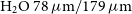
tracing atomic and ionised material at lower excitation temperatures (i.e., below 2 000 K) than probed by optical forbidden lines. SMI, with its high spectral resolution and sensitivity, will break new ground in the study of gas dispersal in protoplanetary disks. Figure 7 shows that SMI/HR can spectrally resolve the the expected photoevaporative wind line profiles as well as detect shifts in the peak and line asymmetries.
$17.43\,\mu\mathrm{m}$
tracing atomic and ionised material at lower excitation temperatures (i.e., below 2 000 K) than probed by optical forbidden lines. SMI, with its high spectral resolution and sensitivity, will break new ground in the study of gas dispersal in protoplanetary disks. Figure 7 shows that SMI/HR can spectrally resolve the the expected photoevaporative wind line profiles as well as detect shifts in the peak and line asymmetries.
Figure 7. Expected profiles of the [Ne II]
 $12.8\mu\mathrm{m}$
(red), [Ne III]
$12.8\mu\mathrm{m}$
(red), [Ne III]
 $15.5\mu\mathrm{m}$
(blue), and [Fe II]
$15.5\mu\mathrm{m}$
(blue), and [Fe II]
 $17.9\mu\mathrm{m}$
(green) lines excited in a X-ray-induced photoevaporative wind, based on the models of Picogna et al. (Reference Picogna, Ercolano, Owen and Weber2019) and the calculations of Weber et al. (Reference Weber, Ercolano, Picogna, Hartmann and Rodenkirch2020). Histograms show how the lines are seen by the SMI instrument. An iron abundance 10 times smaller than solar has been assumed, taking into account the expected Fe depletion onto dust grains.
$17.9\mu\mathrm{m}$
(green) lines excited in a X-ray-induced photoevaporative wind, based on the models of Picogna et al. (Reference Picogna, Ercolano, Owen and Weber2019) and the calculations of Weber et al. (Reference Weber, Ercolano, Picogna, Hartmann and Rodenkirch2020). Histograms show how the lines are seen by the SMI instrument. An iron abundance 10 times smaller than solar has been assumed, taking into account the expected Fe depletion onto dust grains.
Pioneering studies with ground observations at high (
 $R=17\,000$
) resolution with VLT/VISIR have revealed the potential of [Ne II], at
$R=17\,000$
) resolution with VLT/VISIR have revealed the potential of [Ne II], at
 $12.8\,\mu\mathrm{m}$
, as a key diagnostic tracer of photoevaporative winds, where Ne ionisation occurs by the action of both X-ray and UV photons from the central star and the accretion shocks (e.g., Pascucci et al. Reference Pascucci2007; Reference Pascucci2011; Baldovin-Saavedra et al. Reference Baldovin-Saavedra, Audard, Carmona, Güdel, Briggs, Rebull, Skinner and Ercolano2012). The limited observations performed with VISIR have shown that this line usually comes as a single component, and that high-resolution (
$12.8\,\mu\mathrm{m}$
, as a key diagnostic tracer of photoevaporative winds, where Ne ionisation occurs by the action of both X-ray and UV photons from the central star and the accretion shocks (e.g., Pascucci et al. Reference Pascucci2007; Reference Pascucci2011; Baldovin-Saavedra et al. Reference Baldovin-Saavedra, Audard, Carmona, Güdel, Briggs, Rebull, Skinner and Ercolano2012). The limited observations performed with VISIR have shown that this line usually comes as a single component, and that high-resolution (
 $R > 20\,000$
) is needed to discriminate its origin in slow disk winds (
$R > 20\,000$
) is needed to discriminate its origin in slow disk winds (
 $v \sim 5{-}10\,\mathrm{km\ s}^{-1}$
), in the high-velocity jet (
$v \sim 5{-}10\,\mathrm{km\ s}^{-1}$
), in the high-velocity jet (
 $v > 20{-}50\,\mathrm{km\ s}^{-1}$
), or in the inner gaseous disk.
$v > 20{-}50\,\mathrm{km\ s}^{-1}$
), or in the inner gaseous disk.
Molecular line diagnostics originate from regions located at greater distances from the star, that is,
 $1{-}10\,\mathrm{au}$
. Near-IR ro-vibrational lines trace gas temperatures
$1{-}10\,\mathrm{au}$
. Near-IR ro-vibrational lines trace gas temperatures
 $>\!1\,000\,\mathrm{K}$
and probe regions in the disk
$>\!1\,000\,\mathrm{K}$
and probe regions in the disk
 $\sim\!0.5{-}5\,\mathrm{au}$
(gas and dust can thermally de-couple where these lines originate). Spectrally and spatially resolved observations of
$\sim\!0.5{-}5\,\mathrm{au}$
(gas and dust can thermally de-couple where these lines originate). Spectrally and spatially resolved observations of
 $\mathrm{H}_2$
in the near-IR have shown that the emission most often comes from wide-angle low-velocity winds; however, evidence for emission from bound gas in the inner disk has been also found (e.g., Bary et al. Reference Bary, Weintraub and Kastner2003; Beck et al. Reference Beck, Bary, Dutrey, Piétu, Guilloteau, Lubow and Simon2012).
$\mathrm{H}_2$
in the near-IR have shown that the emission most often comes from wide-angle low-velocity winds; however, evidence for emission from bound gas in the inner disk has been also found (e.g., Bary et al. Reference Bary, Weintraub and Kastner2003; Beck et al. Reference Beck, Bary, Dutrey, Piétu, Guilloteau, Lubow and Simon2012).
 $\mathrm{H}_2$
mid-IR lines originate from a region further out, of the order of
$\mathrm{H}_2$
mid-IR lines originate from a region further out, of the order of
 $5{-}10\,\mathrm{au}$
, at
$5{-}10\,\mathrm{au}$
, at
 $T=150{-}1\,000\,\mathrm{K}$
at the disk surface and thus have the unique potential of tracing the gas within the giant planet formation region. Emissions from
$T=150{-}1\,000\,\mathrm{K}$
at the disk surface and thus have the unique potential of tracing the gas within the giant planet formation region. Emissions from
 $\mathrm{H}_2$
mid-IR rotational lines have been searched for in many T Tauri and Herbig sources (from ground-based telescopes and from space); however, positive detections have been obtained only for an handful of objects, mostly via the space-based Spitzer-IRS instrument at low spectral resolution (e.g., Lahuis et al. Reference Lahuis, van Dishoeck, Blake, Evans Neal, Kessler-Silacci and Pontoppidan2007) and thus without the possibility to separate the disk wind contribution from the overall emission. Indeed, models of
$\mathrm{H}_2$
mid-IR rotational lines have been searched for in many T Tauri and Herbig sources (from ground-based telescopes and from space); however, positive detections have been obtained only for an handful of objects, mostly via the space-based Spitzer-IRS instrument at low spectral resolution (e.g., Lahuis et al. Reference Lahuis, van Dishoeck, Blake, Evans Neal, Kessler-Silacci and Pontoppidan2007) and thus without the possibility to separate the disk wind contribution from the overall emission. Indeed, models of
 $\mathrm{H}_2$
emission from disks (e.g., Nomura et al. Reference Nomura, Aikawa, Tsujimoto, Nakagawa and Millar2007) predict flux levels below the detection limit of present instrumentation, but well above the sensitivity limit of SMI. Significantly, a detailed modelling of theses molecular lines using a thermo-chemical treatment for optically thin disk winds is still lacking. Combined, spectrally resolved observations of both near-IR and mid-IR molecular lines should have the potential of tracing the gas temperature stratification of the inner disk.
$\mathrm{H}_2$
emission from disks (e.g., Nomura et al. Reference Nomura, Aikawa, Tsujimoto, Nakagawa and Millar2007) predict flux levels below the detection limit of present instrumentation, but well above the sensitivity limit of SMI. Significantly, a detailed modelling of theses molecular lines using a thermo-chemical treatment for optically thin disk winds is still lacking. Combined, spectrally resolved observations of both near-IR and mid-IR molecular lines should have the potential of tracing the gas temperature stratification of the inner disk.
In the infrared, high-resolution spectra (e.g., VLT/VISIR and CRIRES+, and in the future E-ELT/METIS and TMT/MICHI) can provide very high spectral resolution, but with poorer flux sensitivity than SMI, mainly due to water vapour in the Earth atmosphere and the high thermal background due to the Earth’s atmosphere. Thus, SMI/HR fills a niche ideal to probe, at high spectral resolution, both molecular and atomic lines that trace the disk wind. Furthermore, SMI will probe disk winds across a very large sample of many hundred planet-forming disks, Ideally, the same sample will be observed as undertaken by the disk gas mass survey with SAFARI, providing a census of both the disk conditions and the disk wind properties that cannot be obtained with ground-based observations.
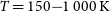
4. Tracing the gas in Debris disks—Volatile content of planetesimals
Gas that is found in debris disk systems is generally thought to be secondary, released from the debris produced in collisions between planetesimals, rather than a direct remnant from the initial star-forming nebula (e.g., Roberge et al. Reference Roberge, Feldman, Weinberger, Deleuil and Bouret2006; Matrà et al. Reference Matrà, Panić and Wyatt2015; Kral Reference Kral2016). As such, this secondary gas provides a unique opportunity to study indirectly the composition of the debris (i.e., the volatile/ice content), and hence the planetesimals, the building blocks of planets. In our Solar System, meteorites (carbonaceous chondrites) contain up to 15 weight% waterFootnote b and water dominates the volatile content in comets (
 $>\!50$
%, Alexander et al. Reference Alexander, McKeegan and Altwegg2018). Hydrous silicates have also been confirmed in C-complex asteroids by AKARI (Usui et al. Reference Usui, Hasegawa, Ootsubo and Onaka2019) and by the sample return missions for Ryugu (Kitazato et al. Reference Kitazato2019) and Bennu (Hamilton et al. Reference Hamilton2019), both of which are C-type asteroids. It is unclear whether extrasolar systems contain similar levels of water and volatiles or whether they are generally drier than the Solar System.
$>\!50$
%, Alexander et al. Reference Alexander, McKeegan and Altwegg2018). Hydrous silicates have also been confirmed in C-complex asteroids by AKARI (Usui et al. Reference Usui, Hasegawa, Ootsubo and Onaka2019) and by the sample return missions for Ryugu (Kitazato et al. Reference Kitazato2019) and Bennu (Hamilton et al. Reference Hamilton2019), both of which are C-type asteroids. It is unclear whether extrasolar systems contain similar levels of water and volatiles or whether they are generally drier than the Solar System.
Planetesimals that were formed far enough from the star, in regions of the protoplanetary disk that are sufficiently cold, are expected to have a significant volatile component. For example, comets in the Solar System are made up by mass of
 $\sim\!50$
%
$\sim\!50$
%
 $\mathrm{H}_2\mathrm{O}$
and
$\mathrm{H}_2\mathrm{O}$
and
 $3{-}10$
% CO (Bockelée-Morvan & Biver Reference Bockelée-Morvan and Biver2017). The volatiles locked inside planetesimals may play a key role in the development of life on exoplanets, since these volatiles can be released from the planetesimals and then migrate to the planets and be captured into their atmospheres (Kral et al. Reference Kral, Davoult and Charnay2020a) or be released upon direct impact with the planet, potentially delivering water, a key ingredient in the origin of life as we know it, and replenishing a secondary atmosphere (Chyba et al. Reference Chyba, Thomas, Brookshaw and Sagan1990; Kral et al. Reference Kral, Wyatt, Triaud, Marino, Thébault and Shorttle2018; Wyatt et al. Reference Wyatt, Kral and Sinclair2020). Understanding this volatile content can also help inform how and where in planet-forming disks planetesimals are able to form; it is for example suggested that planetesimal belts form preferentially at ice lines (Matrà et al. Reference Matrà, Wilner, Öberg, Andrews, Loomis, Wyatt and Dent2018) which should be reflected in a relatively high volatile content in that localised region. Of particular interest is the C/O abundance ratio (Öberg et al. Reference Öberg, Murray-Clay and Bergin2011; Helling et al. Reference Helling, Woitke, Rimmer, Kamp, Thi and Meijerink2014; Moriarty, Madhusudhan, & Fischer Reference Moriarty, Madhusudhan and Fischer2014), since the formation of solids and ultimately planets is believed to be sensitively dependent on this ratio. This is directly due to the fact that the condensation sequence forming solids changes dramatically at
$3{-}10$
% CO (Bockelée-Morvan & Biver Reference Bockelée-Morvan and Biver2017). The volatiles locked inside planetesimals may play a key role in the development of life on exoplanets, since these volatiles can be released from the planetesimals and then migrate to the planets and be captured into their atmospheres (Kral et al. Reference Kral, Davoult and Charnay2020a) or be released upon direct impact with the planet, potentially delivering water, a key ingredient in the origin of life as we know it, and replenishing a secondary atmosphere (Chyba et al. Reference Chyba, Thomas, Brookshaw and Sagan1990; Kral et al. Reference Kral, Wyatt, Triaud, Marino, Thébault and Shorttle2018; Wyatt et al. Reference Wyatt, Kral and Sinclair2020). Understanding this volatile content can also help inform how and where in planet-forming disks planetesimals are able to form; it is for example suggested that planetesimal belts form preferentially at ice lines (Matrà et al. Reference Matrà, Wilner, Öberg, Andrews, Loomis, Wyatt and Dent2018) which should be reflected in a relatively high volatile content in that localised region. Of particular interest is the C/O abundance ratio (Öberg et al. Reference Öberg, Murray-Clay and Bergin2011; Helling et al. Reference Helling, Woitke, Rimmer, Kamp, Thi and Meijerink2014; Moriarty, Madhusudhan, & Fischer Reference Moriarty, Madhusudhan and Fischer2014), since the formation of solids and ultimately planets is believed to be sensitively dependent on this ratio. This is directly due to the fact that the condensation sequence forming solids changes dramatically at
 $\mathrm{C/O}\,\sim\!0.98$
(Larimer Reference Larimer1975). Also, this ratio determines the C/O in primary atmospheres which originate from the accretion of remnant disk material (Massol et al. Reference Massol2016). The C/O ratio also has an impact on secondary atmospheres, as these depend on the bulk planet composition.
$\mathrm{C/O}\,\sim\!0.98$
(Larimer Reference Larimer1975). Also, this ratio determines the C/O in primary atmospheres which originate from the accretion of remnant disk material (Massol et al. Reference Massol2016). The C/O ratio also has an impact on secondary atmospheres, as these depend on the bulk planet composition.
A new technique for probing the volatile content of planetesimals has recently been developed by studying gas in the debris disks found around nearby stars (these are the exo-Kuiper belts found around
 $\sim\!20$
% of stars). The planetesimals collide and are ground down into dust, observable through infrared emission from the dust itself. This process has been studied extensively over the last few decades (e.g., Wyatt Reference Wyatt2008). In this process, the volatiles are also released as gas. The [C I]
$\sim\!20$
% of stars). The planetesimals collide and are ground down into dust, observable through infrared emission from the dust itself. This process has been studied extensively over the last few decades (e.g., Wyatt Reference Wyatt2008). In this process, the volatiles are also released as gas. The [C I]
 $610\,\mu\mathrm{m}$
fine structure line and the CO sub-mm lines have been detected by ALMA from debris disks, revealing the spatial distribution of the gas (e.g., Cataldi et al. Reference Cataldi2018; Moór et al. Reference Moór2019) and in some cases strong asymmetries possibly attributed to recent collisions (e.g., Dent et al. Reference Dent2014, for the case of
$610\,\mu\mathrm{m}$
fine structure line and the CO sub-mm lines have been detected by ALMA from debris disks, revealing the spatial distribution of the gas (e.g., Cataldi et al. Reference Cataldi2018; Moór et al. Reference Moór2019) and in some cases strong asymmetries possibly attributed to recent collisions (e.g., Dent et al. Reference Dent2014, for the case of
 $\beta\,\mathrm{Pic}$
).
$\beta\,\mathrm{Pic}$
).
Assuming the gas is released in a steady-state process, the production rates of CO and dust can then provide their relative quantities in the planetesimals. The systems studied to date, for example, HD 181327 and Fomalhaut, have CO-to-dust compositions that are comparable with Solar System comets (e.g., Marino et al. Reference Marino2016; Matrà et al. Reference Matrà2017). However, Kral et al. (Reference Kral, Matrà, Kennedy, Marino and Wyatt2020b) report two systems that may have less CO than Solar System comets. While the CO content of the planetesimals can be probed in the above way with ALMA, this technique relies on an assumption that the gas is produced in steady state and that the lifetime of CO is set by photodissociation via the interstellar radiation field with, in some cases, CO self-shielding (Visser, van Dishoeck, & Black Reference Visser, van Dishoeck and Black2009; Heays, Bosman, & van Dishoeck Reference Heays, Bosman and van Dishoeck2017). Yet we expect that once CO is destroyed, the C and O atoms will accumulate until they spread through viscous processes to eventually accrete onto the star. Observations of [C I] with ALMA show that in some cases there is sufficient carbon to shield the CO from photodissociating (see Figure 8, Kral et al. Reference Kral, Marino, Wyatt, Kama and Matrà2019). Moreover, the ALMA [C I] observations call into question the steady-state nature of the gas production (Cataldi et al. Reference Cataldi2020) and probably do not probe the bulk of the carbon which is likely to be predominantly ionised, at least for the disks that are not shielded. Cataldi et al. (Reference Cataldi2020) show that a complete knowledge of the gas composition (e.g.,
 $\mathrm{C}^+$
, C, CO) in connection with a detailed photodissociation and ionisation model allows us to time potential large collision events and determine the time since a collisional cascade was initiated. In addition to CO, there may be other volatiles released, in particular
$\mathrm{C}^+$
, C, CO) in connection with a detailed photodissociation and ionisation model allows us to time potential large collision events and determine the time since a collisional cascade was initiated. In addition to CO, there may be other volatiles released, in particular
 $\mathrm{H}_2\mathrm{O}$
which photodissociation turns into OH, H, and O (Kral et al. Reference Kral, Wyatt, Carswell, Pringle, Matrà and Juhász2016). Also here, ALMA observations alone cannot constrain the
$\mathrm{H}_2\mathrm{O}$
which photodissociation turns into OH, H, and O (Kral et al. Reference Kral, Wyatt, Carswell, Pringle, Matrà and Juhász2016). Also here, ALMA observations alone cannot constrain the
 $\mathrm{H}_2\mathrm{O}$
content of the planetesimals since the ‘daughter’ products are only detectable in the far-IR with, for example, SPICA.
$\mathrm{H}_2\mathrm{O}$
content of the planetesimals since the ‘daughter’ products are only detectable in the far-IR with, for example, SPICA.
Figure 8. Sketch of gas distribution in a debris disk based on a detailed dissociation/ionisation model including an interstellar radiation field (IRF). This illustrates the complementarity of ALMA and SPICA gas observations in debris disks. Figure modified from Kral et al. (Reference Kral, Marino, Wyatt, Kama and Matrà2019).
Even though it lacks spectral and spatial resolution, SAFARI is the only instrument that will be able to detect the [O I] lines at 63 and
 $145\,\mu\mathrm{m}$
and use them to measure the atomic oxygen abundance. Another unique line, [C II]
$145\,\mu\mathrm{m}$
and use them to measure the atomic oxygen abundance. Another unique line, [C II]
 $158\,\mu\mathrm{m}$
, is crucial to measure the carbon budget together with ALMA [C I]
$158\,\mu\mathrm{m}$
, is crucial to measure the carbon budget together with ALMA [C I]
 $610\,\mu\mathrm{m}$
and CO sub-mm line measurements. This information is not only relevant for debris disks, but also for planet-forming disks (see Section 2.1). The [C II] line, in conjunction with CO and [C I] observations with ALMA, will allow measurement of the carbon mass, the carbon ionisation fraction, and the electron density in debris disks, all of which constrain both the CO content of the planetesimals and the steady-state versus stochastic production process (as well as the mechanism controlling the viscous evolution, e.g., MRI, Kral & Latter Reference Kral and Latter2016). With this information, the [O I]
$610\,\mu\mathrm{m}$
and CO sub-mm line measurements. This information is not only relevant for debris disks, but also for planet-forming disks (see Section 2.1). The [C II] line, in conjunction with CO and [C I] observations with ALMA, will allow measurement of the carbon mass, the carbon ionisation fraction, and the electron density in debris disks, all of which constrain both the CO content of the planetesimals and the steady-state versus stochastic production process (as well as the mechanism controlling the viscous evolution, e.g., MRI, Kral & Latter Reference Kral and Latter2016). With this information, the [O I]
 $63\,\mu\mathrm{m}$
line flux can be used to determine the
$63\,\mu\mathrm{m}$
line flux can be used to determine the
 $\mathrm{H}_2\mathrm{O}$
content of the planetesimals (see Kral et al. Reference Kral, Wyatt, Carswell, Pringle, Matrà and Juhász2016). In addition, the
$\mathrm{H}_2\mathrm{O}$
content of the planetesimals (see Kral et al. Reference Kral, Wyatt, Carswell, Pringle, Matrà and Juhász2016). In addition, the
 $\mathrm{H}_2\mathrm{O}$
(
$\mathrm{H}_2\mathrm{O}$
(
 $179.7\,\mu\mathrm{m}$
) and OH (
$179.7\,\mu\mathrm{m}$
) and OH (
 $119.3+119.5\,\mu\mathrm{m}$
) lines can be used to probe the water content directly, though detection requires a high production rate due to the short photodissociation time for these molecules (Matrà et al. Reference Matrà, Wilner, Öberg, Andrews, Loomis, Wyatt and Dent2018).
$119.3+119.5\,\mu\mathrm{m}$
) lines can be used to probe the water content directly, though detection requires a high production rate due to the short photodissociation time for these molecules (Matrà et al. Reference Matrà, Wilner, Öberg, Andrews, Loomis, Wyatt and Dent2018).
Previous observations with Herschel (Riviere-Marichalar et al. Reference Riviere-Marichalar2014) only had the sensitivity to detect [O I] and [C II] for a few debris disks, indicated in Figure 9. SAFARI (yellow line) improves significantly on Herschel/PACSFootnote c (red line) and opens the possibility to detect the gas component in a statistically significant sample of debris disks (about 100 potential detections), thereby measuring the volatile content of planetesimals. In addition, these observations characterise the nature of the gas production process, steady versus stochastic, thus informing how the late stages of planet assembly and atmosphere build-up proceed in extrasolar systems (Kral et al. Reference Kral, Davoult and Charnay2020a).
With SAFARI, a
 $\beta$
Pic-equivalent will be detectable with
$\beta$
Pic-equivalent will be detectable with
 $5\,\sigma$
in 1 h out to 150 pc in [O I]
$5\,\sigma$
in 1 h out to 150 pc in [O I]
 $63\,\mu\mathrm{m}$
and 400 pc in [C II]
$63\,\mu\mathrm{m}$
and 400 pc in [C II]
 $158\,\mu\mathrm{m}$
. This increases the volume in which
$158\,\mu\mathrm{m}$
. This increases the volume in which
 $\beta$
Pic-like gas-rich debris disks can be detected 400- to 1200-fold, compared to Herschel/PACS. In this volume, there are hundreds to thousands of debris systems already known (Cotten & Song Reference Cotten, Song, Kastner, Stelzer and Metchev2016), so a careful target selection is possible. To answer the broader question of how the chemical make-up correlates with the stellar spectral type and the presence of planets in the system, linking chemical composition to planet formation, a sample size on the order of 100 systems is required. There are already
$\beta$
Pic-like gas-rich debris disks can be detected 400- to 1200-fold, compared to Herschel/PACS. In this volume, there are hundreds to thousands of debris systems already known (Cotten & Song Reference Cotten, Song, Kastner, Stelzer and Metchev2016), so a careful target selection is possible. To answer the broader question of how the chemical make-up correlates with the stellar spectral type and the presence of planets in the system, linking chemical composition to planet formation, a sample size on the order of 100 systems is required. There are already
 $\sim\!20$
debris disks with CO detected by ALMA, and this number is predicted to continue to rise steadily over the next decade. The detection thresholds for [O I] and [C II] predicted by Kral et al. (Reference Kral, Matrà, Wyatt and Kennedy2017) are comparable to those of ALMA observations of CO and [C I]; this should result in detections of
$\sim\!20$
debris disks with CO detected by ALMA, and this number is predicted to continue to rise steadily over the next decade. The detection thresholds for [O I] and [C II] predicted by Kral et al. (Reference Kral, Matrà, Wyatt and Kennedy2017) are comparable to those of ALMA observations of CO and [C I]; this should result in detections of
 $\sim\!100$
debris disks with both ALMA and SPICA.
$\sim\!100$
debris disks with both ALMA and SPICA.
4.1. Other gas tracers in Debris disks
Other species of importance for planet formation and uniquely available to SPICA are silicon, through the strong [Si II]
 $35\,\mu\mathrm{m}$
line (using SMI), and molecules such as
$35\,\mu\mathrm{m}$
line (using SMI), and molecules such as
 $\mathrm{H}_2\mathrm{O}$
(ortho line at
$\mathrm{H}_2\mathrm{O}$
(ortho line at
 $179.7\,\mu\mathrm{m}$
), and OH (doublet at 119.3,
$179.7\,\mu\mathrm{m}$
), and OH (doublet at 119.3,
 $119.5\,\mu\mathrm{m}$
). Since molecules are quickly dissociated on timescales of days to hundreds of years (see Kral et al. Reference Kral, Marino, Wyatt, Kama and Matrà2019), they will only be found in systems with significant ongoing gas production such as
$119.5\,\mu\mathrm{m}$
). Since molecules are quickly dissociated on timescales of days to hundreds of years (see Kral et al. Reference Kral, Marino, Wyatt, Kama and Matrà2019), they will only be found in systems with significant ongoing gas production such as
 $\beta\,\mathrm{Pic}$
, where CO is observed (Dent et al. Reference Dent2014). Since the molecular lines are likely optically thick, the emission will depend sensitively on the excitation temperature. Assuming a molecular gas distribution similar to the observed CO distribution in the
$\beta\,\mathrm{Pic}$
, where CO is observed (Dent et al. Reference Dent2014). Since the molecular lines are likely optically thick, the emission will depend sensitively on the excitation temperature. Assuming a molecular gas distribution similar to the observed CO distribution in the
 $\beta\,\mathrm{Pic}$
disk (i.e., a solid angle of
$\beta\,\mathrm{Pic}$
disk (i.e., a solid angle of
 $\sim\!1\,\mathrm{arcsec}^2$
at 20 pc), at a velocity dispersion of
$\sim\!1\,\mathrm{arcsec}^2$
at 20 pc), at a velocity dispersion of
 $4\,\mathrm{km\ s}^{-1}$
and excitation temperatures in the range
$4\,\mathrm{km\ s}^{-1}$
and excitation temperatures in the range
 $20{-}85\,\mathrm{K}$
, we find a predicted line flux of
$20{-}85\,\mathrm{K}$
, we find a predicted line flux of
 $\sim\!10^{-18}{-}10^{-17}\,\mathrm{W\,m}^{-2}$
, sufficient to detect
$\sim\!10^{-18}{-}10^{-17}\,\mathrm{W\,m}^{-2}$
, sufficient to detect
 $\mathrm{H}_2\mathrm{O}/\mathrm{OH}$
with
$\mathrm{H}_2\mathrm{O}/\mathrm{OH}$
with
 $5\,\sigma$
in 20 min for a
$5\,\sigma$
in 20 min for a
 $\beta\,\mathrm{Pic}$
-equivalent out to 30–150 pc.
$\beta\,\mathrm{Pic}$
-equivalent out to 30–150 pc.
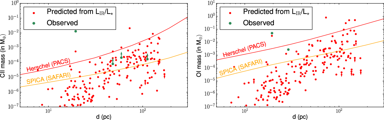
Figure 9. Predicted [C II] (left) and [O I] (right) masses for the sample of 192 debris disks in Kral et al. (Reference Kral, Matrà, Wyatt and Kennedy2017). Approximate detection thresholds for surveys with Herschel/PACS (red, 1 h,
 $5\,\sigma$
) and with SAFARI/HR (yellow, 1 h,
$5\,\sigma$
) and with SAFARI/HR (yellow, 1 h,
 $5\,\sigma$
) are shown; the sensitivity of Herschel was only sufficient to detect (green dots) the most extreme disks in the population in deep integrations (longer than 1 h), whereas with SPICA we can build statistically representative samples of debris disk gas detections. The mass estimates for the few objects that have detections from Herschel are indicated by green dots. Green arrows indicate lower limits of carbon masses related to the large uncertainty on the excitation temperature.
$5\,\sigma$
) are shown; the sensitivity of Herschel was only sufficient to detect (green dots) the most extreme disks in the population in deep integrations (longer than 1 h), whereas with SPICA we can build statistically representative samples of debris disk gas detections. The mass estimates for the few objects that have detections from Herschel are indicated by green dots. Green arrows indicate lower limits of carbon masses related to the large uncertainty on the excitation temperature.
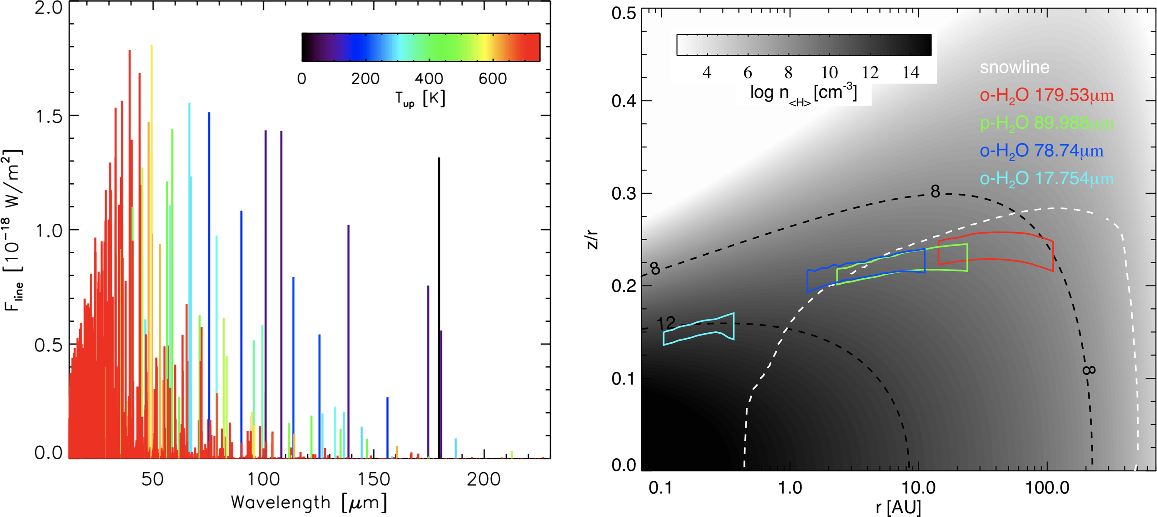
Figure 10. Left: The water vapour line spectra after subtracting the dust continuum, at SMI and SAFARI wavelengths, colour-coded by the energy of the upper levels of the line. Right: The line-emitting regions of various water vapour transitions in a disk around a
 $1\,M_{\odot}$
T Tauri star for the model in Kamp et al. (Reference Kamp, Thi, Woitke, Rab, Bouma and Ménard2017). The white dashed line is the water snowline indicating where water vapor starts to freeze out.
$1\,M_{\odot}$
T Tauri star for the model in Kamp et al. (Reference Kamp, Thi, Woitke, Rab, Bouma and Ménard2017). The white dashed line is the water snowline indicating where water vapor starts to freeze out.
5. The water trail during planet formation
Understanding the water vapour and ice distribution in planet-forming disks will provide information on the origin of water in planetary systems, including our Solar System. Water can be delivered to rocky planets, including Earth, through icy pebbles, icy planetesimals, comets, and asteroids, supporting the emergence of life on these planets.
Water vapour line emission has been detected from protoplanetary disks using ground-based telescopes at near-infrared wavelength (e.g., Carr et al. Reference Carr, Tokunaga and Najita2004). Resolved water line profiles confirmed that they originate in the inner few au of T Tauri disks (Salyk et al. Reference Salyk, Blake, Boogert and Brown2011b; Banzatti et al. Reference Banzatti, Pontoppidan, Salyk, Herczeg, van Dishoeck and Blake2017). The Spitzer Space Telescope detected water vapour lines towards dozens of T Tauri disks (e.g., Carr & Najita Reference Carr and Najita2008; Pontoppidan et al. Reference Pontoppidan, Salyk, Blake, Meijerink, Carr and Najita2010; Salyk et al. Reference Salyk, Pontoppidan, Blake, Najita and Carr2011a). More recently, the Herschel Space Observatory detected warm (
 $\sim\!1\,000\,\mathrm{K}$
) and cold water vapour (
$\sim\!1\,000\,\mathrm{K}$
) and cold water vapour (
 $\sim\!50\,\mathrm{K}$
) in a few disks around T Tauri and Herbig stars (e.g., Hogerheijde et al. Reference Hogerheijde2011; Meeus et al. Reference Meeus2012; Riviere-Marichalar et al. Reference Riviere-Marichalar2012; Fedele et al. Reference Fedele, Bruderer, van Dishoeck, Herczeg, Evans, Bouwman, Henning and Green2012). Meanwhile, near-infrared absorption features of water ice have been detected towards some edge-on disks (e.g., Pontoppidan et al. Reference Pontoppidan, Dullemond, van Dishoeck, Blake, Boogert, Evans Neal, Kessler-Silacci and Lahuis2005; Aikawa et al. Reference Aikawa2012; Terada & Tokunaga Reference Terada and Tokunaga2017) and in scattered light towards some face-on disks (Honda et al. Reference Honda2009; Reference Honda2016) using ground-based telescopes. In addition, far-infrared emission features of water ice have been detected by the ISO and the Herschel Space Observatory towards T Tauri and Herbig disks (e.g., Malfait et al. Reference Malfait, Waelkens, Bouwman, de Koter and Waters1999; McClure et al. Reference McClure2012; Reference McClure2015; Min, Hovenier et al. Reference Min2016b).
$\sim\!50\,\mathrm{K}$
) in a few disks around T Tauri and Herbig stars (e.g., Hogerheijde et al. Reference Hogerheijde2011; Meeus et al. Reference Meeus2012; Riviere-Marichalar et al. Reference Riviere-Marichalar2012; Fedele et al. Reference Fedele, Bruderer, van Dishoeck, Herczeg, Evans, Bouwman, Henning and Green2012). Meanwhile, near-infrared absorption features of water ice have been detected towards some edge-on disks (e.g., Pontoppidan et al. Reference Pontoppidan, Dullemond, van Dishoeck, Blake, Boogert, Evans Neal, Kessler-Silacci and Lahuis2005; Aikawa et al. Reference Aikawa2012; Terada & Tokunaga Reference Terada and Tokunaga2017) and in scattered light towards some face-on disks (Honda et al. Reference Honda2009; Reference Honda2016) using ground-based telescopes. In addition, far-infrared emission features of water ice have been detected by the ISO and the Herschel Space Observatory towards T Tauri and Herbig disks (e.g., Malfait et al. Reference Malfait, Waelkens, Bouwman, de Koter and Waters1999; McClure et al. Reference McClure2012; Reference McClure2015; Min, Hovenier et al. Reference Min2016b).
Water vapour observations from the ground are intrinsically difficult due to the Earth’s atmosphere and thus limited to very narrow windows of high-excitation water lines and low abundance water isotopologues. The Earth’s atmosphere is opaque to the rotational transitions of water, especially the low-J transitions which trace the bulk of the cold gas reservoir in disks. Water remains mostly inaccessible even to air-borne facilities, like SOFIA.
SPICA will characterise the main reservoirs of warm and cold water vapour (see Figure 10) and the far-infrared crystalline and amorphous water ice features, giving unique access to the time evolution of the water throughout the entire disk. SPICA will trace the time evolution of the water snowlines in the planet-forming disks which divide the regions between rocky and gas giant planet formation (Notsu et al. Reference Notsu, Nomura, Ishimoto, Walsh, Honda, Hirota and Millar2016; Reference Notsu, Nomura, Ishimoto, Walsh, Honda, Hirota and Millar2017). SPICA will characterise how the water vapour and ice reservoirs change in the presence of strong accretion events and substructures such as the inner cavities, gaps/rings, and spiral arms, which are related to the disk evolution and planet formation. SPICA will enable the water trail to be traced into the phase of mature planetary systems.
5.1. Tracing the water vapour and ice reservoir
Together, SAFARI and SMI cover a wide range of wavelength and many water vapour emission lines from the mid- to far-IR, as well as water ice features at far-IR wavelengths (45 and
 $63\,\mu\mathrm{m}$
). In particular, the wavelength range of 30–50
$63\,\mu\mathrm{m}$
). In particular, the wavelength range of 30–50
 $\mu\mathrm{m}$
opens new spectroscopic windows with SPICA. SAFARI and SMI provide access to more than a thousand ro-vibrational water vapour transitions spanning a wide range of excitation energies from
$\mu\mathrm{m}$
opens new spectroscopic windows with SPICA. SAFARI and SMI provide access to more than a thousand ro-vibrational water vapour transitions spanning a wide range of excitation energies from
 $E_{\rm up} \sim\!100\,\mathrm{K}$
to several 1 000 K (Figure 10, left). Given this wide range of the energy levels, these transitions are ideal to trace the gaseous reservoirs in a variety of regions within planet-forming disks. Figure 10 (right) shows the dominant emitting regions for four
$E_{\rm up} \sim\!100\,\mathrm{K}$
to several 1 000 K (Figure 10, left). Given this wide range of the energy levels, these transitions are ideal to trace the gaseous reservoirs in a variety of regions within planet-forming disks. Figure 10 (right) shows the dominant emitting regions for four
 $\mathrm{H}_2\mathrm{O}$
transitions in a planet-forming disk around a
$\mathrm{H}_2\mathrm{O}$
transitions in a planet-forming disk around a
 $1\,M_{\odot}$
T Tauri star: the
$1\,M_{\odot}$
T Tauri star: the
 $\mathrm{H}_2\mathrm{O}$
transitions in the SMI/SAFARI wavelength range originate at different radial location in the disk.
$\mathrm{H}_2\mathrm{O}$
transitions in the SMI/SAFARI wavelength range originate at different radial location in the disk.
SPICA has a sensitivity which is a factor of 50 higher than that of either the Spitzer Space Telescope or the Herschel Space Observatory. This enables the detection of both water vapour and ice with disks across a variety of evolutionary stages. Figure 11 shows the flux from the 179.5-
 $\mu\mathrm{m}$
water vapour line as a function of the underlying dust continuum flux, for models with a variety of parameters such as the gas-to-dust mass ratio, the stellar luminosity, and the disk mass (DENT grid, Woitke et al. Reference Woitke, Pinte, Tilling, Ménard, Kamp, Thi, Duchêne and Augereau2010; Kamp et al. Reference Kamp, Woitke, Pinte, Tilling, Thi, Menard, Duchene and Augereau2011). The sensitivity levels of SPICA/SAFARI are shown for shallow and deep surveys, revealing that the water vapour line emission from disks with dust continuum fluxes above
$\mu\mathrm{m}$
water vapour line as a function of the underlying dust continuum flux, for models with a variety of parameters such as the gas-to-dust mass ratio, the stellar luminosity, and the disk mass (DENT grid, Woitke et al. Reference Woitke, Pinte, Tilling, Ménard, Kamp, Thi, Duchêne and Augereau2010; Kamp et al. Reference Kamp, Woitke, Pinte, Tilling, Thi, Menard, Duchene and Augereau2011). The sensitivity levels of SPICA/SAFARI are shown for shallow and deep surveys, revealing that the water vapour line emission from disks with dust continuum fluxes above
 $1\,\mathrm{Jy}$
are detectable. The embedded histogram of dust continuum fluxes for a sample of disks observed by the Herschel Space Observatory reveals that there exists sufficient detectable targets in nearby star-forming regions. The fluxes of various water vapour lines are plotted in Figure 10 (left), showing that many of the lines will be detectable together with the 179.5-
$1\,\mathrm{Jy}$
are detectable. The embedded histogram of dust continuum fluxes for a sample of disks observed by the Herschel Space Observatory reveals that there exists sufficient detectable targets in nearby star-forming regions. The fluxes of various water vapour lines are plotted in Figure 10 (left), showing that many of the lines will be detectable together with the 179.5-
 $\mu\mathrm{m}$
line. Thus, SAFARI and SMI have the potential to trace the evolution of the distribution of water vapour in disks.
$\mu\mathrm{m}$
line. Thus, SAFARI and SMI have the potential to trace the evolution of the distribution of water vapour in disks.
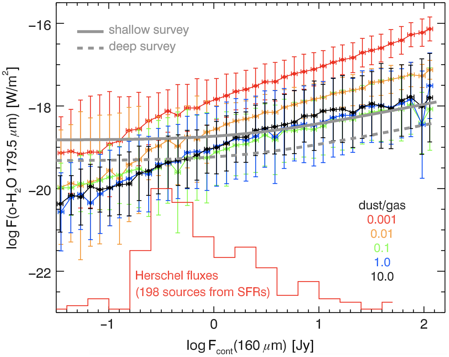
Figure 11. The 179.5-
 $\mu\mathrm{m}$
water vapour line fluxes as a function of the dust continuum fluxes for the DENT grid of disk models with a variety of parameters (Woitke et al. Reference Woitke, Pinte, Tilling, Ménard, Kamp, Thi, Duchêne and Augereau2010; Kamp et al. Reference Kamp, Woitke, Pinte, Tilling, Thi, Menard, Duchene and Augereau2011). The sensitivity levels of SAFARI for a 1 h (shallow) and 10 h (deep) survey and the histogram of observed Herschel dust continuum fluxes (red) from selected star-forming regions are also shown.
$\mu\mathrm{m}$
water vapour line fluxes as a function of the dust continuum fluxes for the DENT grid of disk models with a variety of parameters (Woitke et al. Reference Woitke, Pinte, Tilling, Ménard, Kamp, Thi, Duchêne and Augereau2010; Kamp et al. Reference Kamp, Woitke, Pinte, Tilling, Thi, Menard, Duchene and Augereau2011). The sensitivity levels of SAFARI for a 1 h (shallow) and 10 h (deep) survey and the histogram of observed Herschel dust continuum fluxes (red) from selected star-forming regions are also shown.
5.2. Tracing the water snowlines
The high-resolution mode of SMI is unique for locating the water snowline near the midplane in planet-forming disks. Since the line emission is Doppler-shifted due to the Keplerian rotation, the velocity profiles of the water lines are sensitive to the radial distribution of the water line-emitting region within the disks. SMI/HR (
 $R \sim 30,000$
) spectra enable us to spectroscopically resolve the water line profiles originating in the inner few au of the disk and thus locate kinematically the line-emitting regions, that is, the water snowlines in disks (Figure 12, see also Figure 10 showing the 17.75-
$R \sim 30,000$
) spectra enable us to spectroscopically resolve the water line profiles originating in the inner few au of the disk and thus locate kinematically the line-emitting regions, that is, the water snowlines in disks (Figure 12, see also Figure 10 showing the 17.75-
 $\mu\mathrm{m}$
line-emitting region is located inside the white dashed snowline). Since water vapour is distributed not only inside the water snowline, but also in the warm (a few 100 K) surface layer and the cold outer regions (Figure 12, see also Figure 10 showing the 78.74 and
$\mu\mathrm{m}$
line-emitting region is located inside the white dashed snowline). Since water vapour is distributed not only inside the water snowline, but also in the warm (a few 100 K) surface layer and the cold outer regions (Figure 12, see also Figure 10 showing the 78.74 and
 $179.53\,\mu\mathrm{m}$
lines trace the outer disk), we need to select specific transitions in order to only trace the water vapour inside the water snowline.
$179.53\,\mu\mathrm{m}$
lines trace the outer disk), we need to select specific transitions in order to only trace the water vapour inside the water snowline.
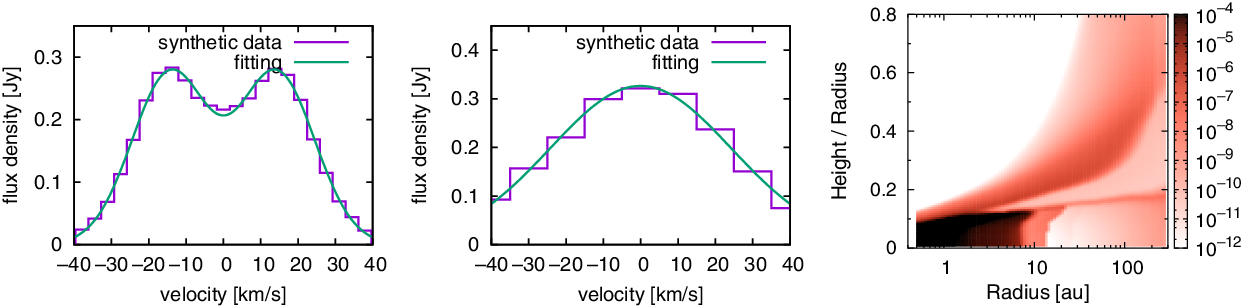
Figure 12. (Left:) Water profiles of the 17.75-
 $\mu\mathrm{m}$
line convolved with
$\mu\mathrm{m}$
line convolved with
 $R=29,000$
(
$R=29,000$
(
 $\Delta v \sim 10\,\mathrm{km\ s}^{-1}$
) and (centre) the 37.98-
$\Delta v \sim 10\,\mathrm{km\ s}^{-1}$
) and (centre) the 37.98-
 $\mu\mathrm{m}$
line convolved with
$\mu\mathrm{m}$
line convolved with
 $R=10,000$
(
$R=10,000$
(
 $\Delta v \sim 30\,\mathrm{km\ s}^{-1}$
), emitted from a Herbig Ae disk with inclination angle of
$\Delta v \sim 30\,\mathrm{km\ s}^{-1}$
), emitted from a Herbig Ae disk with inclination angle of
 $45^\circ$
at a distance of 140 pc. An integration time of
$45^\circ$
at a distance of 140 pc. An integration time of
 $\sim\!10\ \mathrm{min}$
is assumed. (Right:) The
$\sim\!10\ \mathrm{min}$
is assumed. (Right:) The
 $\textbf{water vapour abundance distribution}$
(
$\textbf{water vapour abundance distribution}$
(
 $n_{\rm H_2O}/n_{\rm H}$
) in a disk around a
$n_{\rm H_2O}/n_{\rm H}$
) in a disk around a
 $2.5\ \mathrm{M}_{\odot}$
Herbig Ae star (Notsu et al. Reference Notsu, Nomura, Ishimoto, Walsh, Honda, Hirota and Millar2017)
$2.5\ \mathrm{M}_{\odot}$
Herbig Ae star (Notsu et al. Reference Notsu, Nomura, Ishimoto, Walsh, Honda, Hirota and Millar2017)
Sophisticated physical and chemical disk models show that the transitions with low emissivity, that is, low Einstein A coefficient of
 $10^{-6}{-}10^{-3}\ \mathrm{s}^{-1}$
, and an excitation energy of
$10^{-6}{-}10^{-3}\ \mathrm{s}^{-1}$
, and an excitation energy of
 $E_{\rm up}\sim 1\,000\,\mathrm{K}$
are suitable to trace the water snowline (Notsu et al. Reference Notsu, Nomura, Ishimoto, Walsh, Honda, Hirota and Millar2016; Notsu et al. Reference Notsu, Nomura, Ishimoto, Walsh, Honda, Hirota and Millar2017). These transitions exist at wavelengths ranging from mid-IR to sub-millimetre, and the
$E_{\rm up}\sim 1\,000\,\mathrm{K}$
are suitable to trace the water snowline (Notsu et al. Reference Notsu, Nomura, Ishimoto, Walsh, Honda, Hirota and Millar2016; Notsu et al. Reference Notsu, Nomura, Ishimoto, Walsh, Honda, Hirota and Millar2017). These transitions exist at wavelengths ranging from mid-IR to sub-millimetre, and the
 $17.75\,\mu\mathrm{m}$
line, which satisfies the condition to trace the water snowline, is the best candidate transition in the wavelength range of SMI/HR (
$17.75\,\mu\mathrm{m}$
line, which satisfies the condition to trace the water snowline, is the best candidate transition in the wavelength range of SMI/HR (
 $12{-}18\,\mu\mathrm{m}$
). The
$12{-}18\,\mu\mathrm{m}$
). The
 $37.98\,\mu\mathrm{m}$
line in the wavelength range of SAFARI is similarly suited, but the spectral resolution even with the FTS is lower (
$37.98\,\mu\mathrm{m}$
line in the wavelength range of SAFARI is similarly suited, but the spectral resolution even with the FTS is lower (
 $R \sim 10\,000$
). Thus, SAFARI will not be able to resolve the double peak structure of this emission line but will enable us to measure the line width. This will give us additional information on the location of the snowline (Figure 12).
$R \sim 10\,000$
). Thus, SAFARI will not be able to resolve the double peak structure of this emission line but will enable us to measure the line width. This will give us additional information on the location of the snowline (Figure 12).
These water lines cannot be accessed from ground-based telescopes due to telluric absorption. The sensitivity of the Spitzer Space Telescope was not high enough to detect these lines (Antonellini et al. Reference Antonellini2015; Reference Antonellini2016; Antonellini Reference Antonellini2016). JWST will be able to detect the 17.75-
 $\mu\mathrm{m}$
line, but its highest spectral resolution (
$\mu\mathrm{m}$
line, but its highest spectral resolution (
 $R \sim 3\,000$
) is not high enough to resolve the line profiles. However, JWST observations will be key in measuring line strengths, a key input for the planning of future observations by SPICA. Suitable water lines to trace snowlines with ALMA require long integration times to detect the line profiles (Carr et al. Reference Carr, Najita and Salyk2018; Notsu et al. Reference Notsu, Nomura, Walsh, Honda, Hirota, Akiyama and Millar2018; Reference Notsu2019) and thus it will not be possible to study the time evolution of the location of water snowlines across large samples of disks.
$R \sim 3\,000$
) is not high enough to resolve the line profiles. However, JWST observations will be key in measuring line strengths, a key input for the planning of future observations by SPICA. Suitable water lines to trace snowlines with ALMA require long integration times to detect the line profiles (Carr et al. Reference Carr, Najita and Salyk2018; Notsu et al. Reference Notsu, Nomura, Walsh, Honda, Hirota, Akiyama and Millar2018; Reference Notsu2019) and thus it will not be possible to study the time evolution of the location of water snowlines across large samples of disks.
The detection of the 17.75-
 $\mu\mathrm{m}$
water line profiles towards Herbig Ae stars with enough sensitivity to locate the snowline requires only short integration times (
$\mu\mathrm{m}$
water line profiles towards Herbig Ae stars with enough sensitivity to locate the snowline requires only short integration times (
 $\sim\!30\,\mathrm{min}$
) with SMI/HR even if the disks are located at the distance of the Orion Molecular Clouds (
$\sim\!30\,\mathrm{min}$
) with SMI/HR even if the disks are located at the distance of the Orion Molecular Clouds (
 $\sim\!420\,\mathrm{pc}$
). T Tauri disks in nearby star-forming regions (
$\sim\!420\,\mathrm{pc}$
). T Tauri disks in nearby star-forming regions (
 $<\!300\,\mathrm{pc}$
) will require typically
$<\!300\,\mathrm{pc}$
) will require typically
 $\sim\!1\,\mathrm{h}$
exposure times to achieve the required sensitivity for a reliable snowline estimate.
$\sim\!1\,\mathrm{h}$
exposure times to achieve the required sensitivity for a reliable snowline estimate.
5.3. Tracing the thermal history of water ice
Water ice has multiple bands in the infrared, each of which are sensitive to the temperature of the ice. In the far-IR, two prominent features exist around
 $45\,\mu\mathrm{m}$
and
$45\,\mu\mathrm{m}$
and
 $63\,\mu\mathrm{m}$
. The thermal history of water ice is imprinted in the peak strength and shape of the
$63\,\mu\mathrm{m}$
. The thermal history of water ice is imprinted in the peak strength and shape of the
 $45\,\mu\mathrm{m}$
feature that is narrower in the crystalline phase compared to the amorphous form. In situ formation and mass transport from the inner disk has been discussed by Min et al. (Reference Min, Rab, Woitke, Dominik and Ménard2016a) as potential origin of crystalline water ice in planet-forming disks. Such mixing of material between hot inner regions and cold outer regions of the disks has been also discussed based on the presence of crystalline silicates in comets (e.g., Watson et al. Reference Watson2009).
$45\,\mu\mathrm{m}$
feature that is narrower in the crystalline phase compared to the amorphous form. In situ formation and mass transport from the inner disk has been discussed by Min et al. (Reference Min, Rab, Woitke, Dominik and Ménard2016a) as potential origin of crystalline water ice in planet-forming disks. Such mixing of material between hot inner regions and cold outer regions of the disks has been also discussed based on the presence of crystalline silicates in comets (e.g., Watson et al. Reference Watson2009).
Observing water bands in the far-IR also allows to trace deeper regions within planet-forming disk due to the lower opacity at longer wavelengths. The mid-IR ice bands at 3, 6, and
 $13\,\mu\mathrm{m}$
are mostly optically thick under typical disk conditions and therefore do not probe the reservoir where most of the ice is located (Rocha & Pilling Reference Rocha and Pilling2020). Hence, the 45-
$13\,\mu\mathrm{m}$
are mostly optically thick under typical disk conditions and therefore do not probe the reservoir where most of the ice is located (Rocha & Pilling Reference Rocha and Pilling2020). Hence, the 45-
 $\mu\mathrm{m}$
feature is an excellent tracer of the formation of ice and transport of icy material within disks. Water ice formed in the warm region near the snowline and transported to the cold outer region (cooldown) has a different structure (and thus spectral appearance) compared to water ice formed in cold regions and transported into warm regions (warmup, e.g., Smith et al. Reference Smith, Robinson, Hyland and Carpenter1994). The model calculations around a
$\mu\mathrm{m}$
feature is an excellent tracer of the formation of ice and transport of icy material within disks. Water ice formed in the warm region near the snowline and transported to the cold outer region (cooldown) has a different structure (and thus spectral appearance) compared to water ice formed in cold regions and transported into warm regions (warmup, e.g., Smith et al. Reference Smith, Robinson, Hyland and Carpenter1994). The model calculations around a
 $0.7\,M_{\odot}$
T Tauri star show that ice features with these different thermal histories are distinguishable through observations with a spectral resolution of
$0.7\,M_{\odot}$
T Tauri star show that ice features with these different thermal histories are distinguishable through observations with a spectral resolution of
 $R=250$
(Figure 13). SOFIA/HIRMES also will be able to detect this ice feature; however, SOFIA will require long exposure times,
$R=250$
(Figure 13). SOFIA/HIRMES also will be able to detect this ice feature; however, SOFIA will require long exposure times,
 $\sim\!1\ \mathrm{hr}$
for the most nearby star-forming regions. SPICA/SAFARI can achieve the same sensitivity with much shorter integration times (
$\sim\!1\ \mathrm{hr}$
for the most nearby star-forming regions. SPICA/SAFARI can achieve the same sensitivity with much shorter integration times (
 ${\sim}10\ \mathrm{min}$
) and thus will be a unique instrument to perform large surveys of water ice features towards young objects in various evolutionary stages (Kamp et al. Reference Kamp, Antonellini, Carmona, Ilee, Rab, Ootsubo, Yamamura, Murata and Onaka2018).
${\sim}10\ \mathrm{min}$
) and thus will be a unique instrument to perform large surveys of water ice features towards young objects in various evolutionary stages (Kamp et al. Reference Kamp, Antonellini, Carmona, Ilee, Rab, Ootsubo, Yamamura, Murata and Onaka2018).
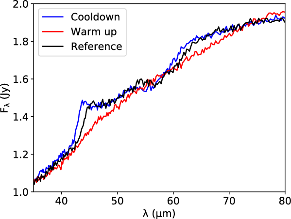
Figure 13. Simulated water ice spectra at
 $45\,\mu\mathrm{m}$
with different thermal histories. Using a 10-min integration (SAFARI noise level) and spectral resolution of
$45\,\mu\mathrm{m}$
with different thermal histories. Using a 10-min integration (SAFARI noise level) and spectral resolution of
 $R=250$
, these are distinguishable. The ‘Reference’ case is for using constant temperature crystalline ice opacities (140 K).
$R=250$
, these are distinguishable. The ‘Reference’ case is for using constant temperature crystalline ice opacities (140 K).
6. From pristine dust to planetesimals/comets
While only 1% of the matter in disks is solid, dust grains play a crucial role in the formation of planetary systems. In order to understand the properties of planets, it is important to constrain the chemical composition of their building blocks: these are small dust particles that enter the disk from the molecular cloud and grow as they are transported inwards. In the inner disk, annealing of the amorphous interstellar grains causes the lattice structure to become ordered, forming crystalline silicates.
Crystalline grains can also be produced by gas phase condensation. Radial mixing transports these hot grains from the inner disk outwards, and they become part of planetesimals and eventually planets. In the inner disk, collisions between dust particles result in a constant cycling of grains between larger and smaller particles, including larger parent bodies. Collisions dominate in the gas-poor debris disk environment, allowing a unique view on the composition of parent bodies. All these processes alter the chemical composition of dust. Infrared spectroscopy can be used to constrain the chemical composition of dust particles.
ISO-SWS, Spitzer-IRS, and JWST-MIRI have studied or will study the dust emission from the inner, warmer disk regions, probing temperatures down to about 100–150 K. The ISO and Spitzer observations show clear evidence for grain growth and the presence of both Mg-rich olivines (
 $\mathrm{Mg}_{2x}\mathrm{Fe}_{(2-2x)}\mathrm{SiO}_4$
) and pyroxenes (
$\mathrm{Mg}_{2x}\mathrm{Fe}_{(2-2x)}\mathrm{SiO}_4$
) and pyroxenes (
 $\mathrm{Mg}_{x}\mathrm{Fe}_{1-x}\mathrm{SiO}_3$
), with up to 10% of Fe contained in some of the crystalline pyroxenes (see, Juhász et al. Reference Juhász2010; Sargent et al. Reference Sargent2009). Spitzer spectra also reveal that olivines are more abundant in the outer disk, and pyroxenes in the inner disk (Juhász et al. Reference Juhász2010). Radial mixing models (e.g., Gail Reference Gail2004) suggest an opposite trend, with olivines (specifically forsterite
$\mathrm{Mg}_{x}\mathrm{Fe}_{1-x}\mathrm{SiO}_3$
), with up to 10% of Fe contained in some of the crystalline pyroxenes (see, Juhász et al. Reference Juhász2010; Sargent et al. Reference Sargent2009). Spitzer spectra also reveal that olivines are more abundant in the outer disk, and pyroxenes in the inner disk (Juhász et al. Reference Juhász2010). Radial mixing models (e.g., Gail Reference Gail2004) suggest an opposite trend, with olivines (specifically forsterite
 $\mathrm{Mg}_2\mathrm{SiO}_4$
) more abundant in the inner disk.
$\mathrm{Mg}_2\mathrm{SiO}_4$
) more abundant in the inner disk.
Much less is known about the composition of the cold dust reservoir. Solar system comets that were formed in the outer regions of the proto-solar nebula contain significant amounts of refractory materials (crystalline silicates, FeS) that require high formation temperatures, that are more typical for the inner disk. (e.g., Crovisier et al. Reference Crovisier, Leech, Bockelee-Morvan, Brooke, Hanner, Altieri, Keller and Lellouch1997; Brownlee Reference Brownlee2014; Wooden et al. Reference Wooden, Ishii and Zolensky2017). In contrast, the molecular and volatile content of comets provides strong evidence that these objects never experienced high temperatures (e.g., Calmonte et al. Reference Calmonte2016). The outer regions of the proto-solar nebula may have experienced substantial mixing of solids from high-temperature regions in the disk. However, it is not clear such radial mixing is a common process in the disk during planet formation.
Both ISO-LWS and Herschel have searched for solid-state features in the far-IR spectra of Herbig Ae/Be disks, and they were successful in detecting the 69-
 $\mu\mathrm{m}$
crystalline olivine band (Malfait et al. Reference Malfait, Waelkens, Waters, Vandenbussche, Huygen and de Graauw1998; Bowey et al. Reference Bowey2002; Sturm et al. 2010; Reference Sturm2013; Maaskant et al. Reference Maaskant, de Vries, Min, Waters, Dominik, Molster and Tielens2015, see Figures 14 and 15). For Herbig Ae/Be proto-planetary disks, Sturm et al. (Reference Sturm2013) found eight detections of the 69
$\mu\mathrm{m}$
crystalline olivine band (Malfait et al. Reference Malfait, Waelkens, Waters, Vandenbussche, Huygen and de Graauw1998; Bowey et al. Reference Bowey2002; Sturm et al. 2010; Reference Sturm2013; Maaskant et al. Reference Maaskant, de Vries, Min, Waters, Dominik, Molster and Tielens2015, see Figures 14 and 15). For Herbig Ae/Be proto-planetary disks, Sturm et al. (Reference Sturm2013) found eight detections of the 69
 $\mu\mathrm{m}$
band of, almost pure, forsterite (
$\mu\mathrm{m}$
band of, almost pure, forsterite (
 $\mathrm{Mg}_2\mathrm{SiO}_4$
) in a sample of 32 Herbig Ae/Be disk observations. For debris disks, only one detection of the 69
$\mathrm{Mg}_2\mathrm{SiO}_4$
) in a sample of 32 Herbig Ae/Be disk observations. For debris disks, only one detection of the 69
 $\mu\mathrm{m}$
band was found out of a set of eight observations (de Vries et al. Reference de Vries2012). The observations so far tell us about the diversity of the crystalline silicate abundance in the cold disk region, implying a variety of disk mixing histories. To directly compare with our Solar System radial mixing history, observations of T Tauri stars are required. However, such observations have been limited due to the sensitivity of previous instruments and issues with the pointing and base-line stability over a broad wavelength range.
$\mu\mathrm{m}$
band was found out of a set of eight observations (de Vries et al. Reference de Vries2012). The observations so far tell us about the diversity of the crystalline silicate abundance in the cold disk region, implying a variety of disk mixing histories. To directly compare with our Solar System radial mixing history, observations of T Tauri stars are required. However, such observations have been limited due to the sensitivity of previous instruments and issues with the pointing and base-line stability over a broad wavelength range.
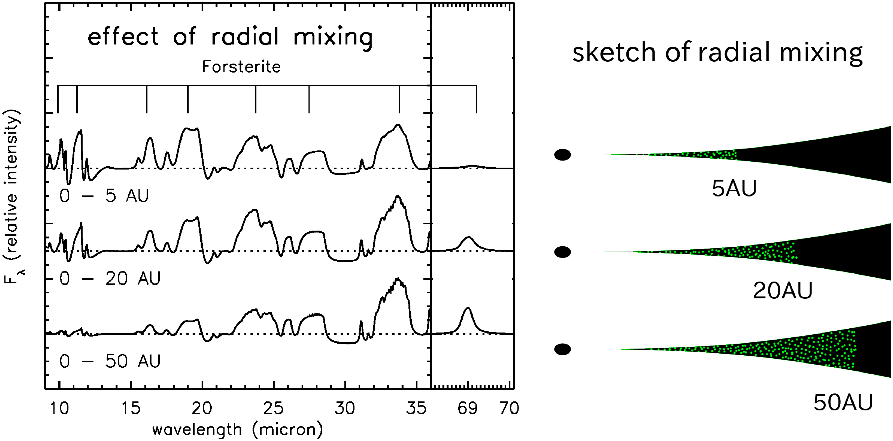
Figure 14. The effect of radial mixing of forsterite (crystalline silicate) grains in the disk on the infrared spectra. When fosterite resides only within 5 au, the
 $69\,\mu\mathrm{m}$
forsterite feature is very weak. On the other hand, when forsterite appears within the 0–50 au radius of the disk, astrong
$69\,\mu\mathrm{m}$
forsterite feature is very weak. On the other hand, when forsterite appears within the 0–50 au radius of the disk, astrong
 $69\,\mu\mathrm{m}$
feature appears (Maaskant et al. Reference Maaskant, de Vries, Min, Waters, Dominik, Molster and Tielens2015).
$69\,\mu\mathrm{m}$
feature appears (Maaskant et al. Reference Maaskant, de Vries, Min, Waters, Dominik, Molster and Tielens2015).
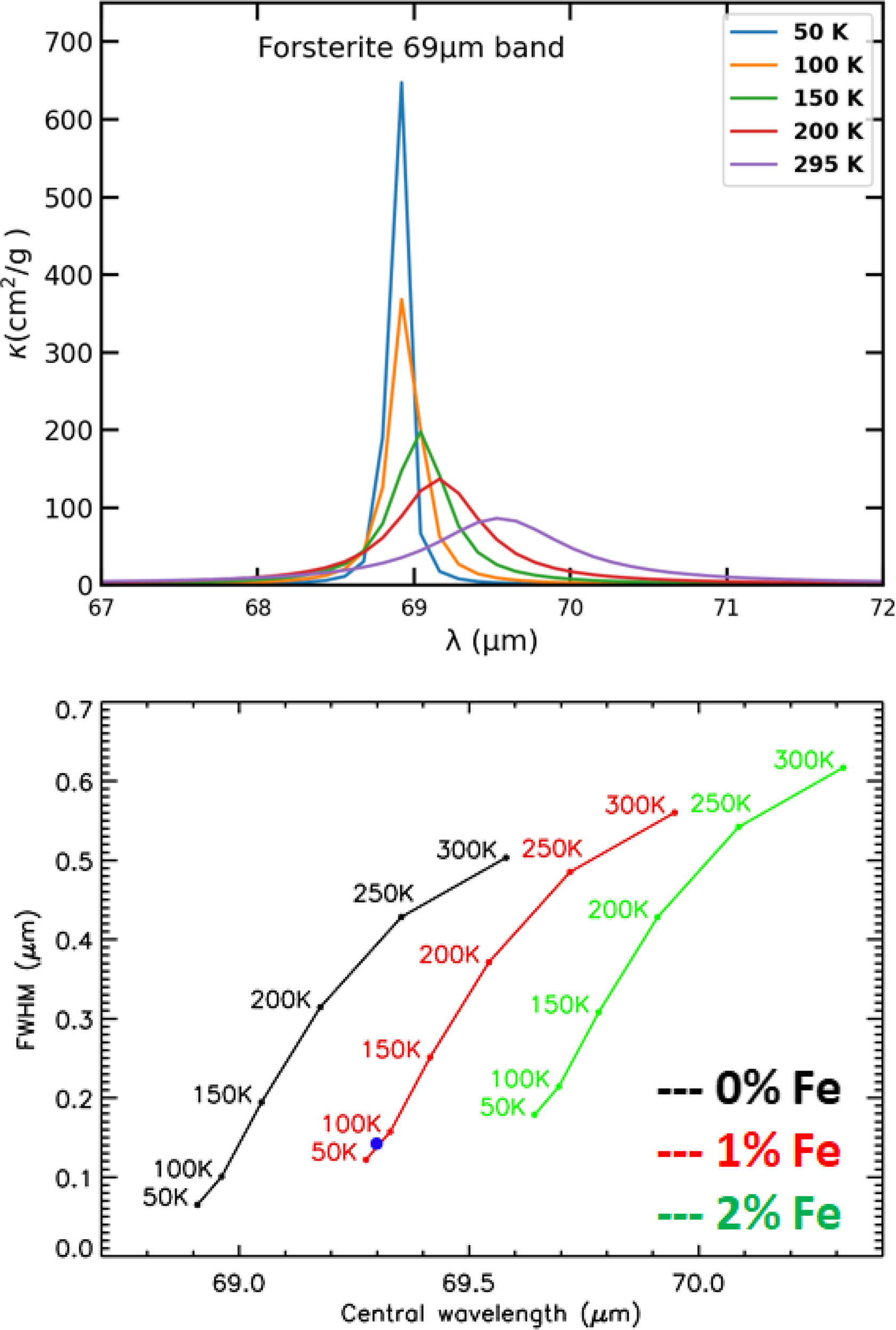
Figure 15. (Top) The 69-
 $\mu\mathrm{m}$
resonance of
$\mu\mathrm{m}$
resonance of
 $\mathrm{Mg}_2\mathrm{SiO}_4$
for a range of temperatures. The band position broadens and shifts redwards with increasing temperature. Note that the band also shifts redwards with increasing Fe content. Optical constants from Suto et al. Reference Suto2006, using a distribution of hollow spheres (DHS) grain model (Min et al. Reference Min, Hovenier and de Koter2005) with
$\mathrm{Mg}_2\mathrm{SiO}_4$
for a range of temperatures. The band position broadens and shifts redwards with increasing temperature. Note that the band also shifts redwards with increasing Fe content. Optical constants from Suto et al. Reference Suto2006, using a distribution of hollow spheres (DHS) grain model (Min et al. Reference Min, Hovenier and de Koter2005) with
 $f=0.7$
and a grain size of
$f=0.7$
and a grain size of
 $1\,\mu\mathrm{m}$
. (Bottom) Forsterite 69-
$1\,\mu\mathrm{m}$
. (Bottom) Forsterite 69-
 $\mu\mathrm{m}$
feature peak and Full Width Half Maximum (FWHM) dependence on Fe content in olivine (
$\mu\mathrm{m}$
feature peak and Full Width Half Maximum (FWHM) dependence on Fe content in olivine (
 $\mathrm{Mg}_{2x}\mathrm{Fe}_{(2-2x)}\mathrm{SiO}_4$
) and temperature. Only 1% inclusion results in
$\mathrm{Mg}_{2x}\mathrm{Fe}_{(2-2x)}\mathrm{SiO}_4$
) and temperature. Only 1% inclusion results in
 $\sim\!0.3\,\mu\mathrm{m}$
shift to longer wavelengths (this figure has been modified from de Vries et al. Reference de Vries2012, Springer Nature).
$\sim\!0.3\,\mu\mathrm{m}$
shift to longer wavelengths (this figure has been modified from de Vries et al. Reference de Vries2012, Springer Nature).
SPICA will be able to observe solid-state resonances from dust particles in the far-IR with unprecedented sensitivity and will have the full mid- to far-IR spectral coverage to identify and characterise minerals that show vibrational resonances over a wide wavelength range (Figure 16). Far-IR resonances of minerals are invaluable since they allow the determination of mineral properties within the low-temperature regions where comets are formed. By using the many resonances of these dust species, the spatial distribution of olivines and pyroxenes can be derived. Figure 14 illustrates how FIR is important to understand the radial mixing history. The relative abundance of olivines to pyroxenes as a function of radius in the disk can be used as a probe of the relative importance of different processes in the disk that produce crystalline silicates, such as chemical equilibrium gas-phase condensation, thermal annealing of molecular cloud amorphous silicates, and (local) flash heating events caused by activities such as stellar outbursts, lightning, and planet formation.
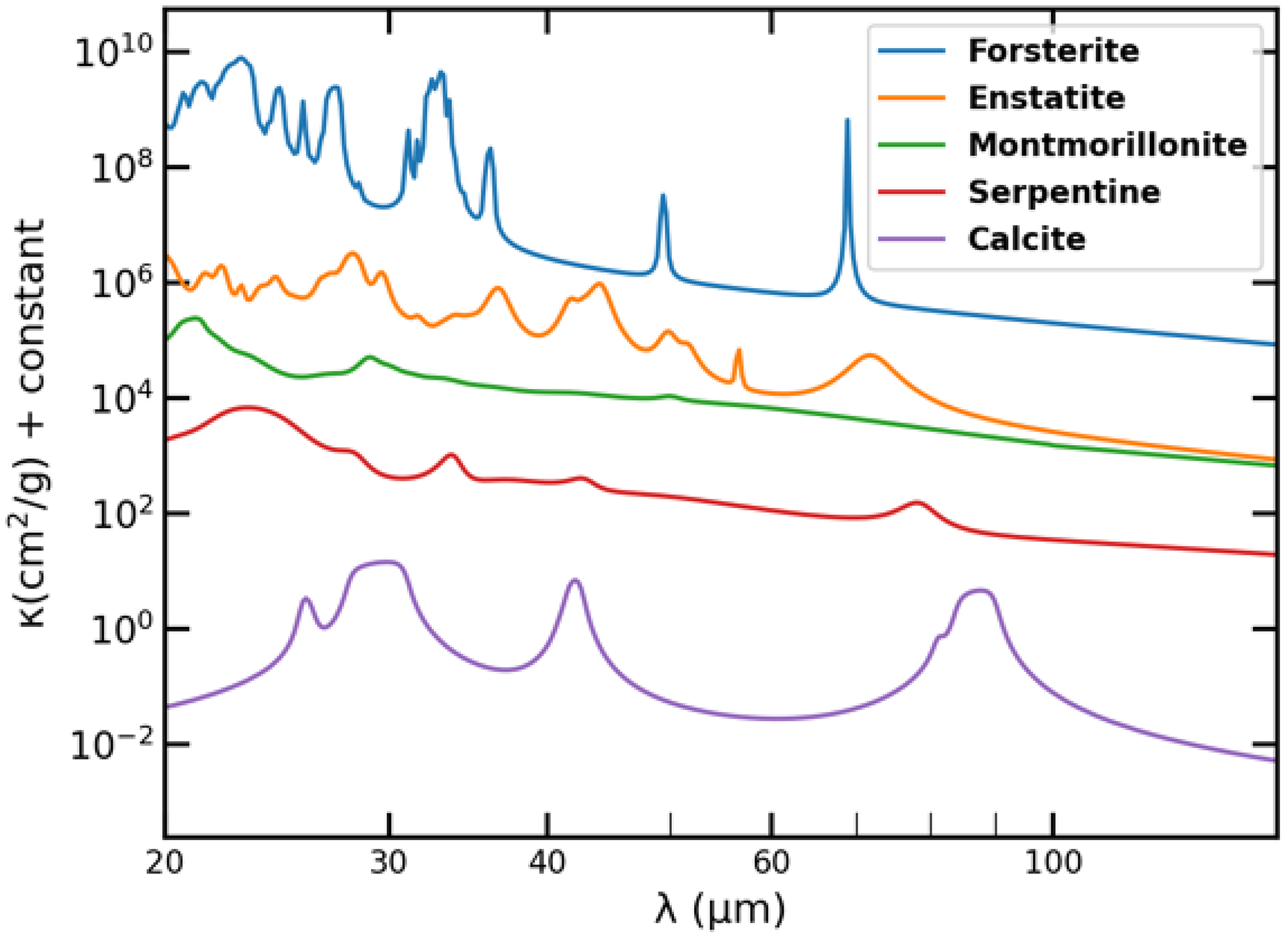
Figure 16. Opacities of forsterite, enstatite, calcite, and the hydrosilicates montmorillonite and serpentine, showing the potential of SPICA to detect these dust species over the full SMI and SAFARI wavelength range. Optical constants from Suto et al. (Reference Suto2006), Zeidler, Mutschke, and Posch (Reference Zeidler, Mutschke and Posch2015), and Koike & Shibai (Reference Koike and Shibai1990) using a ‘distribution of hollow spheres’ grain model (Min et al. Reference Min, Hovenier and de Koter2005) with a vacuum fraction of
 $f=0.7$
and a grain size of
$f=0.7$
and a grain size of
 $0.1\,\mu\mathrm{m}$
.
$0.1\,\mu\mathrm{m}$
.
Far-infrared resonances also allow us to measure the Fe/Mg ratio in crystalline olivine and pyroxene with very high precision (down to an error of better than a percent). For example, the wavelength position and width of the
 $69\,\mu\mathrm{m}$
band of olivine (
$69\,\mu\mathrm{m}$
band of olivine (
 $\mathrm{Mg}_{2x}\mathrm{Fe}_{(2-2x)}\mathrm{SiO}_4$
), is strongly dependent on the Fe/Mg ratio and grain temperature(see Figure 15). This allows a precise determination of the composition of olivine and pyroxene grains. The Fe/Mg ratio of (crystalline) olivine and pyroxene is sensitive to parent body processing and can be used to constrain the size and formation timescale of parent bodies. In the case of a small parent body
$\mathrm{Mg}_{2x}\mathrm{Fe}_{(2-2x)}\mathrm{SiO}_4$
), is strongly dependent on the Fe/Mg ratio and grain temperature(see Figure 15). This allows a precise determination of the composition of olivine and pyroxene grains. The Fe/Mg ratio of (crystalline) olivine and pyroxene is sensitive to parent body processing and can be used to constrain the size and formation timescale of parent bodies. In the case of a small parent body
 $(\!<\!10\ \mathrm{km}$
), the composition of the mineral is unaltered since its formation in the proto-planetary disk and we expect a very low Fe content (Fe/(Fe + Mg)
$(\!<\!10\ \mathrm{km}$
), the composition of the mineral is unaltered since its formation in the proto-planetary disk and we expect a very low Fe content (Fe/(Fe + Mg)
 $\sim 0$
). In slightly larger parent bodies (
$\sim 0$
). In slightly larger parent bodies (
 $\sim\!10\,\mathrm{km}$
to several hundreds of kilometres), the minerals undergo equilibration (Fe/(Fe + Mg)
$\sim\!10\,\mathrm{km}$
to several hundreds of kilometres), the minerals undergo equilibration (Fe/(Fe + Mg)
 $\sim 0.3$
) and for large planetesimals and planets (
$\sim 0.3$
) and for large planetesimals and planets (
 $>\!200\,\mathrm{km}$
) igneous processes will strongly impact the minerals (Fe/(Fe + Mg)
$>\!200\,\mathrm{km}$
) igneous processes will strongly impact the minerals (Fe/(Fe + Mg)
 $> 0.5$
. As in gas-rich disks, the mineralogy of
$> 0.5$
. As in gas-rich disks, the mineralogy of
 $\mu\mathrm{m}$
-sized dust particles in debris disks directly probes the composition of their parent bodies: extra-solar asteroids and comets.
$\mu\mathrm{m}$
-sized dust particles in debris disks directly probes the composition of their parent bodies: extra-solar asteroids and comets.
Furthermore, a search for carbon-bearing solids such as calcite and dolomite will be interesting. Carbon-bearing minerals like calcite (
 $\mathrm{CaCO}_3$
) and dolomite (CaMg)(
$\mathrm{CaCO}_3$
) and dolomite (CaMg)(
 $\mathrm{CO}_3$
)
$\mathrm{CO}_3$
)
 $_2$
only form under specific conditions, on Earth requiring the presence of liquid water or biogenic processes. Carbonates have been detected in evolved stars (Kemper et al. Reference Kemper, Jäger, Waters, Henning, Molster, Barlow, Lim and de Koter2002) and protostars (Ceccarelli et al. Reference Ceccarelli, Caux, Tielens, Kemper, Waters and Phillips2002). Several formation mechanisms have been proposed (e.g., Toppani et al. Reference Toppani, Robert, Libourel, de Donato, Barres, D’Hendecourt and Ghanbaja2005), such as gas-grain chemical reactions and non-equilibrium gas-phase condensation, all requiring a
$_2$
only form under specific conditions, on Earth requiring the presence of liquid water or biogenic processes. Carbonates have been detected in evolved stars (Kemper et al. Reference Kemper, Jäger, Waters, Henning, Molster, Barlow, Lim and de Koter2002) and protostars (Ceccarelli et al. Reference Ceccarelli, Caux, Tielens, Kemper, Waters and Phillips2002). Several formation mechanisms have been proposed (e.g., Toppani et al. Reference Toppani, Robert, Libourel, de Donato, Barres, D’Hendecourt and Ghanbaja2005), such as gas-grain chemical reactions and non-equilibrium gas-phase condensation, all requiring a
 $\mathrm{CO}_2$
and
$\mathrm{CO}_2$
and
 $\mathrm{H}_2\mathrm{O}$
-rich environment. The detection of such minerals in planetary systems would strongly impact our current view on the early presence of environments that are essential for life.
$\mathrm{H}_2\mathrm{O}$
-rich environment. The detection of such minerals in planetary systems would strongly impact our current view on the early presence of environments that are essential for life.
7. The first true Kuiper belt analogue
While all stars presumably host debris disks at some level, only the thermal continuum of the brightest 20% are currently detectable, and we know neither our rank in the remaining 80%, nor how this rank is related to the Solar System’s history or planetary architecture. A decade from now we will have detected or set stringent limits on planets around most nearby stars, but the limits on small body populations will be as poor as they are now (see Figure 17). SPICA provides our only opportunity to detect true Kuiper belt analogues.
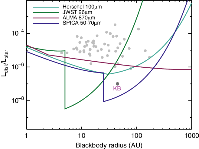
Figure 17. Sensitivity to Kuiper belt analogues at 5 pc. The blackbody radius is the stellocentric radius obtained from the dust temperature by assuming the dust behaves as a blackbody. Grey dots are known disks around nearby stars. Disks that lie above a given instrument’s line are detectable. The SPICA sensitivity at 50–
 $70\,\mu\mathrm{m}$
is very similar, so only one line is shown. Thus, only SPICA can detect debris disks at Kuiper belt (and fainter) levels.
$70\,\mu\mathrm{m}$
is very similar, so only one line is shown. Thus, only SPICA can detect debris disks at Kuiper belt (and fainter) levels.
A true Kuiper belt (KB) analogue is defined here as a debris disk with a fractional luminosity
 $L_{\rm disk}/L_{\star} \sim 10^{-7}$
and a radius of
$L_{\rm disk}/L_{\star} \sim 10^{-7}$
and a radius of
 $\sim\!45\,L_\star^{0.2}\,\mathrm{au}$
(i.e., scaling with
$\sim\!45\,L_\star^{0.2}\,\mathrm{au}$
(i.e., scaling with
 $L_\star$
as suggested by mm-wave imaging of bright debris disks, Matrà et al. Reference Matrà, Wyatt, Wilner, Dent, Marino, Kennedy and Milli2019). With temperatures of
$L_\star$
as suggested by mm-wave imaging of bright debris disks, Matrà et al. Reference Matrà, Wyatt, Wilner, Dent, Marino, Kennedy and Milli2019). With temperatures of
 $\sim\!50\,\mathrm{K}$
, KB analogues emit essentially all of their energy at far-IR wavelengths, but their low luminosities imply that this emission is at most 1% of the stellar flux. To detect a debris disk requires: (1) sensitivity sufficient to detect the disk flux, (2) unresolved disks to be brighter than some fraction of the stellar flux due to calibration uncertainties, (3) resolved disks to have surface brightness greater than the local uncertainty in the stellar Point Spread Function (PSF), and (4) disks to be brighter than the confusion limit. The typical calibration limit (2) is
$\sim\!50\,\mathrm{K}$
, KB analogues emit essentially all of their energy at far-IR wavelengths, but their low luminosities imply that this emission is at most 1% of the stellar flux. To detect a debris disk requires: (1) sensitivity sufficient to detect the disk flux, (2) unresolved disks to be brighter than some fraction of the stellar flux due to calibration uncertainties, (3) resolved disks to have surface brightness greater than the local uncertainty in the stellar Point Spread Function (PSF), and (4) disks to be brighter than the confusion limit. The typical calibration limit (2) is
 $\sim\!10$
%, explaining why it is not possible to detect unresolved KB analogues (e.g., with Spitzer or Herschel), while the sensitivity and PSF limits (1) and (3) preclude the detection of resolved KB analogues with ALMA, JWST, or in scattered light. These points are illustrated in Figure 17 which shows the detectability of debris disks with different radii and fractional luminosities for a Sun-like star at 5 pc. Disks can be detected above the lines indicated for a given instrument, and essentially all known disks lie above the Herschel
$\sim\!10$
%, explaining why it is not possible to detect unresolved KB analogues (e.g., with Spitzer or Herschel), while the sensitivity and PSF limits (1) and (3) preclude the detection of resolved KB analogues with ALMA, JWST, or in scattered light. These points are illustrated in Figure 17 which shows the detectability of debris disks with different radii and fractional luminosities for a Sun-like star at 5 pc. Disks can be detected above the lines indicated for a given instrument, and essentially all known disks lie above the Herschel
 $100\,\mu\mathrm{m}$
limit, with no current or planned instruments able to detect KB analogues, except SPICA.
$100\,\mu\mathrm{m}$
limit, with no current or planned instruments able to detect KB analogues, except SPICA.
This unique capability of SPICA is possible because of its combination of photometric sensitivity and resolution at wavelengths around the peak KB emission. Constraint (2) can be avoided by observing stars close enough that a KB analogue would be resolved (see Figure 18, left panels), and constraint (4) is partially or wholly avoided by observing at
 $\leq\!70\,\mu\mathrm{m}$
, rather than at
$\leq\!70\,\mu\mathrm{m}$
, rather than at
 $100\,\mu\mathrm{m}$
where a KB analogue would be well below the confusion limit. This means that, once the resolution constraint is met, sensitivity (1) and PSF stability (3) constraints on SPICA’s imaging performance determine the number of stars for which it will be feasible to detect true KB analogues, as shown in the right panels of Figure 18. Here we consider surveys at
$100\,\mu\mathrm{m}$
where a KB analogue would be well below the confusion limit. This means that, once the resolution constraint is met, sensitivity (1) and PSF stability (3) constraints on SPICA’s imaging performance determine the number of stars for which it will be feasible to detect true KB analogues, as shown in the right panels of Figure 18. Here we consider surveys at
 $34\,\mu\mathrm{m}$
(upper panels) and
$34\,\mu\mathrm{m}$
(upper panels) and
 $70\,\mu\mathrm{m}$
(lower panels). Both require that the SPICA PSF be very well understood, but the shorter wavelength is preferred as the higher spatial resolution means that more stars can be observed (compare for example the number of stars closer than the resolution limit in the left panels of Figure 18).
$70\,\mu\mathrm{m}$
(lower panels). Both require that the SPICA PSF be very well understood, but the shorter wavelength is preferred as the higher spatial resolution means that more stars can be observed (compare for example the number of stars closer than the resolution limit in the left panels of Figure 18).
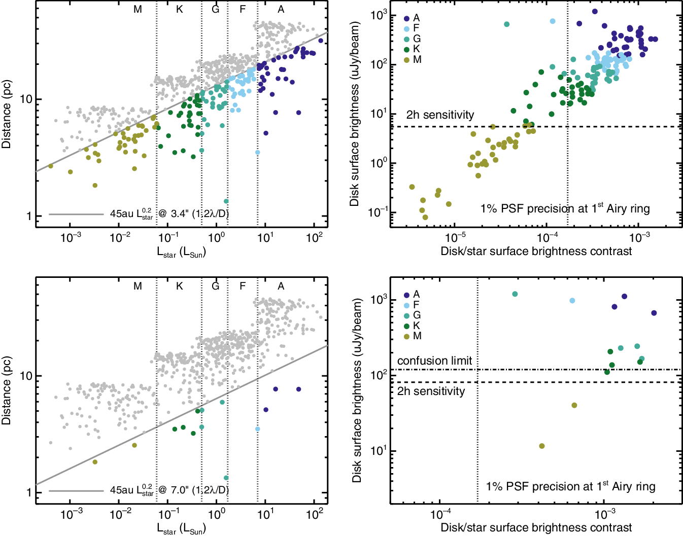
Figure 18. Kuiper Belt sample selection. The top row shows the 34-
 $\mu\mathrm{m}$
SMI survey, and the bottom row shows the 70
$\mu\mathrm{m}$
SMI survey, and the bottom row shows the 70
 $\mu\mathrm{m}$
B-BOP survey. (Left panels:) Volume-limited sample of nearby stars (Phillips et al. 2010). The KBs of targets falling below the solid line would be resolvable by SPICA. (Right panels:) The surface brightness of resolvable KB analogues is used to determine a further selection based on a 3
$\mu\mathrm{m}$
B-BOP survey. (Left panels:) Volume-limited sample of nearby stars (Phillips et al. 2010). The KBs of targets falling below the solid line would be resolvable by SPICA. (Right panels:) The surface brightness of resolvable KB analogues is used to determine a further selection based on a 3
 $\sigma$
detection in a 2-h observation assuming the sensitivity (dashed lines) and confusion limits (dot-dashed lines), and disk to star contrast assuming the PSF is known at 1% accuracy near the first Airy ring (dotted lines). Stars with detectable KBs lie above and right of all lines. Here disks have been assumed to be face-on; inclined disks would move up and to the right on this plot. Detection for the top left target in the upper right panel,
$\sigma$
detection in a 2-h observation assuming the sensitivity (dashed lines) and confusion limits (dot-dashed lines), and disk to star contrast assuming the PSF is known at 1% accuracy near the first Airy ring (dotted lines). Stars with detectable KBs lie above and right of all lines. Here disks have been assumed to be face-on; inclined disks would move up and to the right on this plot. Detection for the top left target in the upper right panel,
 $\alpha$
Cen, should still be possible as the angular size of a KB for this target is well beyond 1.2
$\alpha$
Cen, should still be possible as the angular size of a KB for this target is well beyond 1.2
 $\lambda/D$
. KBs around M-type stars cannot be detected at 34
$\lambda/D$
. KBs around M-type stars cannot be detected at 34
 $\mu\mathrm{m}$
unless the contrast is better than
$\mu\mathrm{m}$
unless the contrast is better than
 $1.7 \times 10^{-4}$
, or at 70
$1.7 \times 10^{-4}$
, or at 70
 $\mu\mathrm{m}$
because their surface brightness is below the confusion limit (unless stellar proper motion is used to subtract the background).
$\mu\mathrm{m}$
because their surface brightness is below the confusion limit (unless stellar proper motion is used to subtract the background).
The sensitivity limit (1) is shown on the right panels of Figure 18 as horizontal dashed lines assuming a 2-h observation per star, and using the nominal sensitivities (e.g.,
 $10\,\mu\mathrm{Jy}$
,
$10\,\mu\mathrm{Jy}$
,
 $5\,\sigma 1\,\mathrm{h}$
for SMI). A longer observation is not warranted at 70
$5\,\sigma 1\,\mathrm{h}$
for SMI). A longer observation is not warranted at 70
 $\mu\mathrm{m}$
because this already reaches the confusion limit (horizontal dash-dot line), while at 34
$\mu\mathrm{m}$
because this already reaches the confusion limit (horizontal dash-dot line), while at 34
 $\mu\mathrm{m}$
the sample is more constrained by the PSF stability. For the PSF stability limit (3), consider that the surface brightness of a star’s first Airy ring is 1.7% of the star. The right panels of Figure 18 show that at both wavelengths face-on KB analogues are 10-100 times fainter than this at a comparable location (though these could be in the minima). Thus to detect such disks, the surface brightness of the PSF wings must be known to
$\mu\mathrm{m}$
the sample is more constrained by the PSF stability. For the PSF stability limit (3), consider that the surface brightness of a star’s first Airy ring is 1.7% of the star. The right panels of Figure 18 show that at both wavelengths face-on KB analogues are 10-100 times fainter than this at a comparable location (though these could be in the minima). Thus to detect such disks, the surface brightness of the PSF wings must be known to
 $\sim\!1$
% accuracy, resulting in a PSF stability requirement of
$\sim\!1$
% accuracy, resulting in a PSF stability requirement of
 $1.7 \times 10^{-4}$
of the peak near the first Airy ring. This is the vertical dotted line shown on the right panels of Figure 18. This PSF stability constraint can be relaxed by a factor of a few at 70
$1.7 \times 10^{-4}$
of the peak near the first Airy ring. This is the vertical dotted line shown on the right panels of Figure 18. This PSF stability constraint can be relaxed by a factor of a few at 70
 $\mu\mathrm{m}$
because the star is fainter but the disk similarly bright compared with the shorter wavelength (meaning that sensitivity, or more accurately confusion is the limiting factor). Assuming that this PSF requirement can be met, surveys at each of the wavelengths would be able to detect KB analogues around the stars in the top right quadrants of the right panels of Figure 18. These limits are somewhat pessimistic in the sense that an inclined KB analogue would have higher surface brightness, and higher disk to star contrast, than assumed.
$\mu\mathrm{m}$
because the star is fainter but the disk similarly bright compared with the shorter wavelength (meaning that sensitivity, or more accurately confusion is the limiting factor). Assuming that this PSF requirement can be met, surveys at each of the wavelengths would be able to detect KB analogues around the stars in the top right quadrants of the right panels of Figure 18. These limits are somewhat pessimistic in the sense that an inclined KB analogue would have higher surface brightness, and higher disk to star contrast, than assumed.
The frequency of Kuiper belt analogues is unknown but might be expected to be several tens of percent. Deriving the incidence with a precision of a few percent, comparable with that for brighter disks, would allow characterisation of the entire brightness distribution down to sub-KB levels, thus placing the Solar System’s debris disk in context for the first time. This level of precision requires observing several tens of stars. Figure 18 left shows that the KBs around
 $>\!100$
nearby stars would have a large enough angular size to be resolved by SPICA at 34
$>\!100$
nearby stars would have a large enough angular size to be resolved by SPICA at 34
 $\mu\mathrm{m}$
, and 14 at 70
$\mu\mathrm{m}$
, and 14 at 70
 $\mu\mathrm{m}$
. Of these, Figure 18 right shows that KB analogues around M-types would be too faint given the sensitivity, confusion, and/or PSF stability limits, leaving an unbiased sample of
$\mu\mathrm{m}$
. Of these, Figure 18 right shows that KB analogues around M-types would be too faint given the sensitivity, confusion, and/or PSF stability limits, leaving an unbiased sample of
 $\sim\!100$
targets at 34
$\sim\!100$
targets at 34
 $\mu\mathrm{m}$
and 11 at 70
$\mu\mathrm{m}$
and 11 at 70
 $\mu\mathrm{m}$
. Furthermore,
$\mu\mathrm{m}$
. Furthermore,
 $\sim\!7$
from the 34
$\sim\!7$
from the 34
 $\mu\mathrm{m}$
sample and 4 from the 70
$\mu\mathrm{m}$
sample and 4 from the 70
 $\mu\mathrm{m}$
sample are already known to host detected disks (i.e., they are in the 20% of the population that have KBs bright enough to be detected by photometry). Thus, while a survey at 70
$\mu\mathrm{m}$
sample are already known to host detected disks (i.e., they are in the 20% of the population that have KBs bright enough to be detected by photometry). Thus, while a survey at 70
 $\mu\mathrm{m}$
could achieve the first detection of a true KB analogue, a survey at 34
$\mu\mathrm{m}$
could achieve the first detection of a true KB analogue, a survey at 34
 $\mu\mathrm{m}$
would be better suited to determining the frequency of dust at KB analogue levels.
$\mu\mathrm{m}$
would be better suited to determining the frequency of dust at KB analogue levels.
Table 2. Summary of the reference mission. Surveys in brackets use the data acquired by the main survey and do not require a different sample and/or longer exposure times. Exposure time estimates are derived using SAFARI simulator version 1.2 issue 6.2 and SMI simulator version 4.
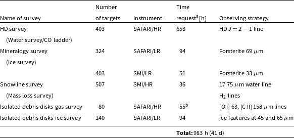
aThis is the exposure time without instrument and observatory overheads.
bThese times were derived using issue 3.0 of the SAFARI time estimator (w/o background).
To summarise, the proposed observing strategy is to image systems at 34 and/or 70
 $\mu\mathrm{m}$
with SMI or B-BOP (if the latter includes a 70-
$\mu\mathrm{m}$
with SMI or B-BOP (if the latter includes a 70-
 $\mu\mathrm{m}$
detector), but the goal of detecting true KB analogues would only be feasible if the above PSF stability constraint can be met.
$\mu\mathrm{m}$
detector), but the goal of detecting true KB analogues would only be feasible if the above PSF stability constraint can be met.
8. A reference observing programme
In the context of the ESA M5 process, we studied the feasibility of achieving the science goals outlined in this paper within the typical lifetime of a space mission. We rely here on the detailed instrument descriptions, wavelength ranges, spectral resolution and sensitivities, outlined in Roelfsema et al. (Reference Roelfsema2018) for the mid- and far-IR instruments SMI (Kaneda et al. Reference Wada2020) and SAFARI (Roelfsema et al. Reference Roelfsema2018) and briefly summarised in the preface.
Table 2 summarises a potential reference observing programme consisting of six surveys with strongly overlapping samples. Details of how the surveys are compiled can be found in Appendix A. These surveys would provide the data required to answer the key science questions outlined in this white paper. The total exposure time required for such a reference programme is 1.5 months. If we add typical overheads such as 10% calibration time, slew times (3 min per source) and assume an overall efficiency of the observatory of 60% (based on Herschel experience), we estimate the full reference observing programme to take
 $\sim\!77\,\mathrm{d}$
, or
$\sim\!77\,\mathrm{d}$
, or
 ${\sim\!2.5}$
months. This is eminently feasible within a mission lifetime of3 yr.
${\sim\!2.5}$
months. This is eminently feasible within a mission lifetime of3 yr.
9. Beyond SPICA
We now let loose the mission design of SPICA and comment in the following subsections on a couple of interesting capabilities that should be considered for future infrared instrumentation development.
9.1. Mid-IR spectral resolution
The spectral resolution of
 $R \sim 30\,000$
is crucial to resolve line profiles from the inner warm disk and to separate the peaks of the Keplerian profiles (see Section A.3). Increasing the resolution further can help disentangling more complex lines profiles (more than two peaks), but the true gain arises once line profiles can fully resolve disk wind kinematic features. Figure 7 shows that the spectral resolution of
$R \sim 30\,000$
is crucial to resolve line profiles from the inner warm disk and to separate the peaks of the Keplerian profiles (see Section A.3). Increasing the resolution further can help disentangling more complex lines profiles (more than two peaks), but the true gain arises once line profiles can fully resolve disk wind kinematic features. Figure 7 shows that the spectral resolution of
 $R \sim 30\,000$
is enough to detect a shift of the wind profile with respect to the disk rest frame. However, a full study of the line asymmetries, including accurate peak determination, arising from various disk dispersal processes warrants a resolution of
$R \sim 30\,000$
is enough to detect a shift of the wind profile with respect to the disk rest frame. However, a full study of the line asymmetries, including accurate peak determination, arising from various disk dispersal processes warrants a resolution of
 $R \sim 100\,000$
, or
$R \sim 100\,000$
, or
 $\sim\!3\,\mathrm{km\ s}^{-1}$
, such as available on the ground with VLT CRIRES.
$\sim\!3\,\mathrm{km\ s}^{-1}$
, such as available on the ground with VLT CRIRES.
9.2. Far-IR spectral resolution
The limited SAFARI spectral resolution will make it difficult to kinematically separate the individual components contributing to the emission lines and thus to isolate the emission within the disk from that in the disk wind and outflow. In practice, it will only be possible to distinguish atomic emission in fast jets, that is,
 $v_{\rm jet} > 50\,\mathrm{km\ s}^{-1}$
, contributing to the [O I] line at
$v_{\rm jet} > 50\,\mathrm{km\ s}^{-1}$
, contributing to the [O I] line at
 $63\,\mu\mathrm{m}$
, where the resolution is
$63\,\mu\mathrm{m}$
, where the resolution is
 $R > 5\,000$
. To properly discriminate between the various components potentially contributing to the far-IR lines (disk, wind), we require a spectral resolution of
$R > 5\,000$
. To properly discriminate between the various components potentially contributing to the far-IR lines (disk, wind), we require a spectral resolution of
 $30\,000$
, close to that which SMI offers at shorter wavelengths.
$30\,000$
, close to that which SMI offers at shorter wavelengths.
9.3. Wavelength coverage
The only water line excited by cold gas in the SAFARI wavelength range is the 179.5
 $\mu\mathrm{m}$
ortho-
$\mu\mathrm{m}$
ortho-
 $\mathrm{H}_2\mathrm{O}$
line (
$\mathrm{H}_2\mathrm{O}$
line (
 $T_{\rm up}=114.4\,\mathrm{K}$
). However, going to slightly longer wavelengths than presently envisioned for SAFARI, the 269.27
$T_{\rm up}=114.4\,\mathrm{K}$
). However, going to slightly longer wavelengths than presently envisioned for SAFARI, the 269.27
 $\mu\mathrm{m}$
para-water line (
$\mu\mathrm{m}$
para-water line (
 $T_{\rm up}=53.43\,\mathrm{K}$
), one of the three ground state lines of water could be included. Furthermore, due to this increase in spectral coverage, the gap in the CO ladder would close with respect to the ground-based sub-millimetre facilities. This would be beneficial for measuring the radial temperature gradients in disks, especially to gain accuracy at the spatial scales of a few to a few 10 au.
$T_{\rm up}=53.43\,\mathrm{K}$
), one of the three ground state lines of water could be included. Furthermore, due to this increase in spectral coverage, the gap in the CO ladder would close with respect to the ground-based sub-millimetre facilities. This would be beneficial for measuring the radial temperature gradients in disks, especially to gain accuracy at the spatial scales of a few to a few 10 au.
9.4. Mirror size
Finally, a larger primary mirror would undoubtedly increase the sensitivity and diminish confusion at far-IR wavelengths. This increase in angular resolution is very interesting for detecting a true Kuiper Belt analogue (Section 7). The higher the spatial resolution, the larger the ‘volume’ and hence potential sample size available for searching for true Kuiper Belt analogues (Figure 18). The most stringent constraint here is in fact the level of PSF stability for far-IR imaging that is required to detect the faint disk emission with sufficient confidence (see Section 7).
10. Conclusions
This white paper describes the unique science questions that a spectroscopic infrared space mission such as SPICA can answer. Mid- to far-IR infrared spectra will uniquely measure the gas masses of disks (HD, CO ladder) and the water/ice content and determine how these evolve during the planet-forming period. The key measurements of infrared lines (e.g., HD, OH, water, mid- to far-IR fine structure lines) will pinpoint the crucial transition when disks exhaust their primordial gas and further planet formation may use secondary gas produced from planetesimals. The mid-IR high spectral resolution is also unique in determining indirectly from the water line profiles the location of the snowline dividing the rocky and icy mass reservoir in the disk and how this evolves during the build-up of planetary systems. Infrared spectroscopy (mid- to far-IR) of key solid state bands (e.g., forsterite, enstatite, hydrosilicates, calcite) is crucial for assessing whether extensive radial mixing, which is part of our Solar System history, is a general process occurring in all planetary systems. The combined gas, dust, and ice observations of debris disks will assess whether extrasolar planetesimals are similar to our Solar System comets/asteroids.
With SPICA being taken out of the M5 competition, there is no other facility within the next 20 yr that will be able to measure these fundamental quantities in statistically relevant samples of planet-forming disks. Among the facilities that the infrared community is constantly pushing forward are the Origins Space TelescopeFootnote d proposed as part of the US Decadal Survey and a potential new instrument on the Stratospheric Observatory for Infrared Astronomy (SOFIA) filling the niche of medium- to high-resolution spectroscopy in the 30–120
 $\mu\mathrm{m}$
wavelength range. This latter instrument would have less sensitivity compared to SPICA but could serve as a key pathfinder for the brighter objects.
$\mu\mathrm{m}$
wavelength range. This latter instrument would have less sensitivity compared to SPICA but could serve as a key pathfinder for the brighter objects.
Acknowledgements
I.K. acknowledges funding from ‘Grants-in-Aid for Scientific Research 25108004’ for a work visit to Japan for discussing the SPICA project and relevant science. M.H. was supported by JSPS KAKENHI Grant Numbers JP17H01103, JP18H05441. M.A. acknowledges support from the Prodex Experiment Arrangement C4000128332 for the Swiss contribution to SPICA. S.N. is grateful for support from JSPS (Japan Society for the Promotion of Science) Overseas Research Fellowships when he belonged to Leiden University, and RIKEN Special Postdoctoral Research Fellowship, and he is supported by MEXT/JSPS Grants-in-Aid for Scientific Research (KAKENHI) 16J06887 and 20K22376. W.R.M.R. acknowledges the support by the European Research Council (ERC) under the European Union’s Horizon 2020 research and innovation programme through ERC Consolidator Grant ‘S4F’ (grant agreement No 646908). B.N. and D.F. acknowledge financial support by the Agenzia Spaziale Italiana (ASI) under the research contract 2018-31-HH.0. D.J is supported by the National Research Council of Canada and by an NSERC Discovery Grant.
A Reference observing programme
The following subsections describe a potential observing programme that would provide the data to answer the research questions raised in the main paper. The source lists have been compiled using the current knowledge and only serve to demonstrate that (a) statistical samples can be compiled and (b) the required observing time remains feasible within a typical mission lifetime of a few years. The disk gas mass case (HD) has been identified as leading and thus the HD survey is largely driving the sample selection also for the mineralogy and snowline case.
We report here observing times without overheads that have been calculated using the instrument simulators of the SAFARI (version 1.2, issue 6.2) and SMI instruments (version 4). Based on the Herschel experience, we could expect an efficiency of 60% and typical slew times of 3 min. We also assume that the calibration time on average amounts to 10% of the observation time.
A.1 HD survey
Experience from past Spitzer and Herschel surveys (e.g., Evans et al. 2009; Reference SturmSturm et al. 2010; Reference DentDent et al. 2013) shows that statistically relevant sample sizes consist of at least 100 sources per age bin (star-forming region). The reason behind this is that even at a specific age/within a Star Forming Region (SFR), there is a large scatter in terms of stellar (e.g., spectral type, mass accretion rate, X-ray luminosity) and disk (e.g., mass, gas-to-dust mass ratio, temperature, surface density) properties.
In order to address the disk gas mass evolution as function of time, we need to observe SFRs with a wide spread of ages and well characterised Young Stellar Object (YSO) populations (Spitzer and Herschel data) covering class I to class III sources. These are shown in Table 3 with their ages, distances, sample sizes, and respective references.
Table 3. Properties of the star-forming regions to be targeted. We propose to select the best 100 targets in each of the five age bins based on the availability of ancillary data and characterisation in the next decade.
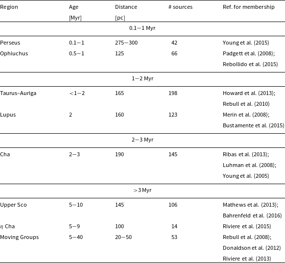
We group them in four age bins:
 $0.1-1\,\mathrm{Myr}$
,
$0.1-1\,\mathrm{Myr}$
,
 $1-2\,\mathrm{Myr}$
,
$1-2\,\mathrm{Myr}$
,
 $2-3\,\mathrm{Myr}$
and older than 3 Myr. These regions will be surveyed in addition by ALMA and JWST in the next decade. ALMA will provide a full census of disk sizes (gas and dust), inclinations and for a few cases in depth characterisation of non-axisymmetric structures (and protoplanets); JWST will provide an inventory of water, ices, and organic molecules inside
$2-3\,\mathrm{Myr}$
and older than 3 Myr. These regions will be surveyed in addition by ALMA and JWST in the next decade. ALMA will provide a full census of disk sizes (gas and dust), inclinations and for a few cases in depth characterisation of non-axisymmetric structures (and protoplanets); JWST will provide an inventory of water, ices, and organic molecules inside
 $\sim\!10\,\mathrm{au}$
.
$\sim\!10\,\mathrm{au}$
.
The final selection of appropriate SFRs should be driven by the largest ancillary datasets (Spitzer, WISE, Herschel, ALMA, and JWST data) and the need for sample diversity. Our strategy here is to cover the entirety of these SFRs and Moving Groups with sample sizes of 100 objects per age bin selected across a stellar mass range. We aim, for 10 bins in stellar mass (from M-dwarfs to F-type stars, logarithmically spaced) and 10 objects per mass bin to cover a representative range of mass accretion rates). This provides the basis for determining the gas dispersal timescale. Within a star-forming region, we probe different evolutionary stages (class I, II, III, transitional disks, disks with substructure from SPHERE, ALMA), mass accretion rates, and stellar spectral types; however, the main focus will be on the class II disks. Within the selected SFRs, we can show which secondary factors such as spectral type, disk size, and mass accretion rates play a role next to SED class and age in setting the gas evolution.
We will select
 $\sim\!20$
class I and II sources in Perseus to capture the earliest stages. From each age bin (see Table 3), we eventually select a total of 100 targets, leading to 400 targets for the reference sample. We note that this is the minimum required to address the gas mass evolution during the planet formation epoch. We expect many additional open-time programmes to build and expand on this. Examples could be to extend this survey to higher stellar masses (intermediate mass T Tau stars and Herbig Ae’s), to add very deep surveys at the low mass end (brown dwarfs), or to add more distant high mass star-forming regions such as Orion.
$\sim\!20$
class I and II sources in Perseus to capture the earliest stages. From each age bin (see Table 3), we eventually select a total of 100 targets, leading to 400 targets for the reference sample. We note that this is the minimum required to address the gas mass evolution during the planet formation epoch. We expect many additional open-time programmes to build and expand on this. Examples could be to extend this survey to higher stellar masses (intermediate mass T Tau stars and Herbig Ae’s), to add very deep surveys at the low mass end (brown dwarfs), or to add more distant high mass star-forming regions such as Orion.
The reference programme thus contains 400 objects (out of the ones listed in Table 3) to be targeted in order to answer the key science questions: (1) How does the disk gas mass evolve through the planet-forming epoch and (2) Which other factors besides age play a role in this evolution.
The goal is line detection; the lines do not need to be spectrally resolved in the SAFARI wavelength range. However, since molecular lines have a very low line-to-continuum ratio (
 $\lesssim\!0.005$
), that is, weak narrow gas lines (unresolved) on a strong continuum, we require the highest possible spectral resolution to maximise the line detection rate. The low excitation HD lines (
$\lesssim\!0.005$
), that is, weak narrow gas lines (unresolved) on a strong continuum, we require the highest possible spectral resolution to maximise the line detection rate. The low excitation HD lines (
 $J=1-0, 2-1$
are expected to have typical widths of
$J=1-0, 2-1$
are expected to have typical widths of
 $5-20\,\mathrm{km\ s}^{-1}$
(depending also on inclination). In the SAFARI wavelength range, a resolving power of
$5-20\,\mathrm{km\ s}^{-1}$
(depending also on inclination). In the SAFARI wavelength range, a resolving power of
 $R\!\gtrsim\!3\,000$
is needed. At a resolution of 2 800, the HD lines are not blended and line fluxes can be extracted in a straightforward manner. Another key transition is the ortho-
$R\!\gtrsim\!3\,000$
is needed. At a resolution of 2 800, the HD lines are not blended and line fluxes can be extracted in a straightforward manner. Another key transition is the ortho-
 $\mathrm{H}_2\mathrm{O}$
 $2_{12}-1_{01}$
line at 179.533
$2_{12}-1_{01}$
line at 179.533
 $\mu\mathrm{m}$
that is very close to the CH
$\mu\mathrm{m}$
that is very close to the CH
 $^+$
$^+$
 $J=2-1$
transition at 179.601
$J=2-1$
transition at 179.601
 $\mu\mathrm{m}$
. In order to deblend the two lines, a resolving power of
$\mu\mathrm{m}$
. In order to deblend the two lines, a resolving power of
 $R\!\gtrsim\!2\,800$
(
$R\!\gtrsim\!2\,800$
(
 $\Delta \lambda \lesssim\!0.036\,\mu\mathrm{m}$
) is needed. A smaller resolving power would not permit to deblend these two lines and to measure the flux of the
$\Delta \lambda \lesssim\!0.036\,\mu\mathrm{m}$
) is needed. A smaller resolving power would not permit to deblend these two lines and to measure the flux of the
 $\mathrm{H}_2\mathrm{O}$
 $2_{12}-1_{01}$
. This line is very important because the 179.533
$2_{12}-1_{01}$
. This line is very important because the 179.533
 $\mu\mathrm{m}$
line is the only transition (in the SAFARI spectral range) that traces the cold water gas reservoir.
$\mu\mathrm{m}$
line is the only transition (in the SAFARI spectral range) that traces the cold water gas reservoir.
At a distance of 140 pc, the expected disk integrated flux of the HD
 $J=1-0$
line ranges from
$J=1-0$
line ranges from
 $\sim\!1\times 10^{-19}\,\mathrm{W\,m}^{-2}$
for
$\sim\!1\times 10^{-19}\,\mathrm{W\,m}^{-2}$
for
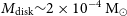 $M_{\rm disk}\!\sim\!2\times 10^{-4}\,\mathrm{M}_{\odot}$
to
$M_{\rm disk}\!\sim\!2\times 10^{-4}\,\mathrm{M}_{\odot}$
to
 $\sim\!1\times 10^{-18}\,\mathrm{W\,m}^{-2}$
for
$\sim\!1\times 10^{-18}\,\mathrm{W\,m}^{-2}$
for
 $M_{\rm disk}=10^{-2}\,\mathrm{M}_{\odot}$
(Trapman et al. Reference Trapman, Miotello, Kama, van Dishoeck and Bruderer2017). The SPICA detection limit of
$M_{\rm disk}=10^{-2}\,\mathrm{M}_{\odot}$
(Trapman et al. Reference Trapman, Miotello, Kama, van Dishoeck and Bruderer2017). The SPICA detection limit of
 $\sim\!1.3\times 10^{-19}\,\mathrm{W\,m}^{-2}$
(1 h, 5
$\sim\!1.3\times 10^{-19}\,\mathrm{W\,m}^{-2}$
(1 h, 5
 $\sigma$
, point-source mode), therefore, will allow us to study the evolution of disks at least down to disk gas masses of
$\sigma$
, point-source mode), therefore, will allow us to study the evolution of disks at least down to disk gas masses of
 $\sim\!3\times 10^{-4}\,\mathrm{M}_{\odot}$
. Disk models and observations indicate a clear correlation between line and continuum fluxes (Figure 19), so that we could expect for stronger continuum sources also on average higher line fluxes. This enables an efficient observing strategy, where the limiting sensitivity for HD is informed by the predicted continuum (from Spitzer, Herschel, ALMA data) at 60 and 100
$\sim\!3\times 10^{-4}\,\mathrm{M}_{\odot}$
. Disk models and observations indicate a clear correlation between line and continuum fluxes (Figure 19), so that we could expect for stronger continuum sources also on average higher line fluxes. This enables an efficient observing strategy, where the limiting sensitivity for HD is informed by the predicted continuum (from Spitzer, Herschel, ALMA data) at 60 and 100
 $\mu\mathrm{m}$
.
$\mu\mathrm{m}$
.
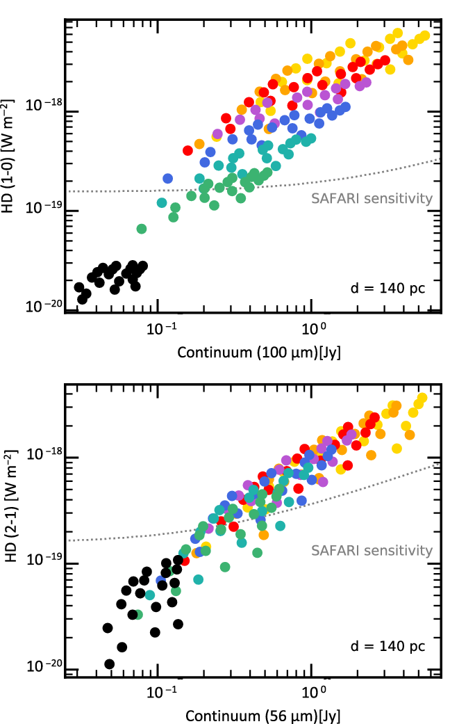
Figure 19. HD line fluxes versus continuum for the grid of models taken from Trapman et al. (Reference Trapman, Miotello, Kama, van Dishoeck and Bruderer2017) assuming a distance of 140 pc. The SAFARI sensitivity curve is displayed as a dashed line for a 1-h integration. The colour scale is the same as in Figure 3.
Also, for the more distant star-forming region, Perseus (factor 2 more distant compared to above estimates), we require a factor 16 longer integration times to reach the
 $M_{\rm disk}\!\sim\!2 \times 10^{-4}\,\mathrm{M}_{\odot}$
mass limit. However, none of the class II targets in that region will be brighter than 0.1 Jy and thus we exploit the full SAFARI sensitivity.
$M_{\rm disk}\!\sim\!2 \times 10^{-4}\,\mathrm{M}_{\odot}$
mass limit. However, none of the class II targets in that region will be brighter than 0.1 Jy and thus we exploit the full SAFARI sensitivity.
Based on the strategy outlined above and a ‘current best’ subselection of targets from Table 3, a deep survey for the gas mass estimates will take a total observing time of 928 h (38.7 d) (integration time of 612.9 h or 25.5 d). In this subselection (see Table 4), class II disks dominate (244), but we retain a statistically significant sample of class I sources (61) for tracking differences in SED evolutionary stage and also a significant sample of class III sources (97) for assessing the transition from primordial to secondary gas, a crucial point in the mode of planet formation; this class III sample also constitutes potentially a fraction of ‘young’ debris disks for which we can study the detailed gas composition (see Section 4).
Table 4. Distribution of classes within the subselected sample for the HD mass survey.
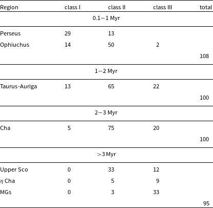
A.2 Mineralogy/Ice survey
The mid- and far-IR spectral region contains many bands of abundant minerals and of water ice (see Figure 16). Table 5 shows the key mid-/far-IR bands covered by SAFARI and SMI. In order to get the full inventory also the mid-IR bands (e.g., forsterite at 23.5 and 33.5
 $\mu\mathrm{m}$
) should be observed with SMI.
$\mu\mathrm{m}$
) should be observed with SMI.
Table 5. Mineral resonances with wavelengths positions above 20
 $\mu\mathrm{m}$
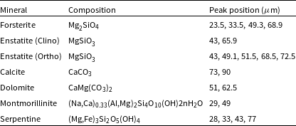
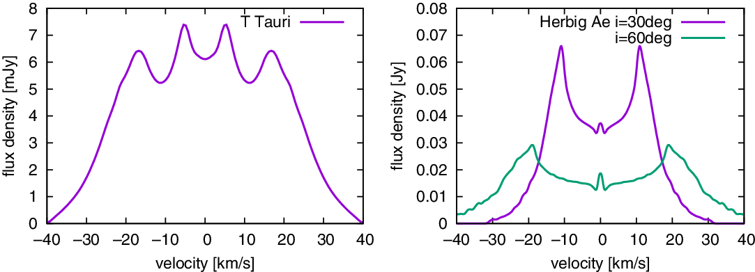
Figure 20. The 17.75-
 $\mu\mathrm{m}$
water line flux densities obtained by model calculations of (left) a T Tauri disk located at 300 pc and (right) a Herbig Ae disk located at 420 pc. The dust continuum is subtracted. References for the T Tauri models: Antonellini et al. (2015; Reference Antonellini2016), for the Herbig Ae models: Notsu et al. (Reference Notsu, Nomura, Ishimoto, Walsh, Honda, Hirota and Millar2016); Notsu et al. (2017; Reference Notsu, Nomura, Walsh, Honda, Hirota, Akiyama and Millar2018)
$\mu\mathrm{m}$
water line flux densities obtained by model calculations of (left) a T Tauri disk located at 300 pc and (right) a Herbig Ae disk located at 420 pc. The dust continuum is subtracted. References for the T Tauri models: Antonellini et al. (2015; Reference Antonellini2016), for the Herbig Ae models: Notsu et al. (Reference Notsu, Nomura, Ishimoto, Walsh, Honda, Hirota and Millar2016); Notsu et al. (2017; Reference Notsu, Nomura, Walsh, Honda, Hirota, Akiyama and Millar2018)
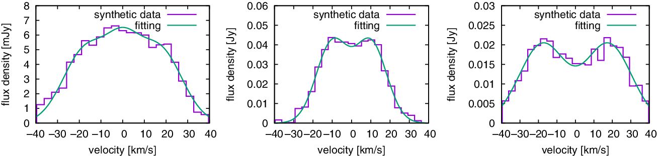
Figure 21. The 17.75-
 $\mu\mathrm{m}$
water line profiles deconvolved with spectral resolution of
$\mu\mathrm{m}$
water line profiles deconvolved with spectral resolution of
 $R=29,000$
and sampling of
$R=29,000$
and sampling of
 $N=1.5$
for a T Tauri disk located at 300 pc (left) and a Herbig Ae disk located at 420 pc with inclination angle of 30
$N=1.5$
for a T Tauri disk located at 300 pc (left) and a Herbig Ae disk located at 420 pc with inclination angle of 30
 $^\circ$
(centre) and 60
$^\circ$
(centre) and 60
 $^\circ$
(right). Noise levels of 0.28 mJy and 1.4 mJy are used for a T Tauri disk model and Herbig Ae disk model, respectively. The synthetic data can be fitted with a double peak profile. The spectral resolution of
$^\circ$
(right). Noise levels of 0.28 mJy and 1.4 mJy are used for a T Tauri disk model and Herbig Ae disk model, respectively. The synthetic data can be fitted with a double peak profile. The spectral resolution of
 $R\!\sim\!30,000$
is required in order to resolve the position of double peaks.
$R\!\sim\!30,000$
is required in order to resolve the position of double peaks.
A Herschel far-IR spectroscopic study was done with 32 Herbig Ae/Be stars, which is a too small sample to disentangle multiple parameters which could drive changes in the mineralogy. We thus want to increase the number of targets to
 $\sim\!400$
to enable a comprehensive statistical study of the evolutionary trend with SPICA. The source sample will be shared for large parts with the HD survey which acquires SAFARI/HR spectroscopy. In addition,
$\sim\!400$
to enable a comprehensive statistical study of the evolutionary trend with SPICA. The source sample will be shared for large parts with the HD survey which acquires SAFARI/HR spectroscopy. In addition,
 $\sim\!100$
debris disk sources should also be observed to see the continuous evolutionary trend from pre-main-sequence stars to main sequence stars. This latter sample is shared with the debris disk gas/ice surveys.
$\sim\!100$
debris disk sources should also be observed to see the continuous evolutionary trend from pre-main-sequence stars to main sequence stars. This latter sample is shared with the debris disk gas/ice surveys.
Most bands are a few
 $\mu\mathrm{m}$
to several tens of
$\mu\mathrm{m}$
to several tens of
 $\mu\mathrm{m}$
wide. However, the Forsterite 69-
$\mu\mathrm{m}$
wide. However, the Forsterite 69-
 $\mu\mathrm{m}$
band shape and peak position carry valuable diagnostic value of Fe content in the olivine structures. For example, 1% inclusion will result in
$\mu\mathrm{m}$
band shape and peak position carry valuable diagnostic value of Fe content in the olivine structures. For example, 1% inclusion will result in
 $\sim\!0.3\,\mu\mathrm{m}$
peak shift to longer wavelengths. To distinguish this shift, it requires a spectral resolution
$\sim\!0.3\,\mu\mathrm{m}$
peak shift to longer wavelengths. To distinguish this shift, it requires a spectral resolution
 $R\!>\!230$
. A spectral resolution of
$R\!>\!230$
. A spectral resolution of
 $>\!230$
is also important because in some spectral ranges vibrational resonances of dust species may blend, such as the enstatite complex near 40–43
$>\!230$
is also important because in some spectral ranges vibrational resonances of dust species may blend, such as the enstatite complex near 40–43
 $\mu\mathrm{m}$
, or the serpentine band near 21
$\mu\mathrm{m}$
, or the serpentine band near 21
 $\mu\mathrm{m}$
that may blend with crystalline forsterite and amorphous silicate (SMI wavelength range). In addition, it is important to have a reliable calibration of the relative spectral response function over a wavelength range allowing the detection of broad (5–10
$\mu\mathrm{m}$
that may blend with crystalline forsterite and amorphous silicate (SMI wavelength range). In addition, it is important to have a reliable calibration of the relative spectral response function over a wavelength range allowing the detection of broad (5–10
 $\mu\mathrm{m}$
) and weak (1–2% above the local continuum) bands. An additional requirement is the calibration of SMI with respect to SAFARI, because dust species have vibrational resonances covering the wavelength ranges of SMI and SAFARI. The relative strengths of the resonances carry information about, for example, the temperature distribution, chemical gradients, and abundance gradients. Band strength ratios should be determined with an accuracy of 5%.
$\mu\mathrm{m}$
) and weak (1–2% above the local continuum) bands. An additional requirement is the calibration of SMI with respect to SAFARI, because dust species have vibrational resonances covering the wavelength ranges of SMI and SAFARI. The relative strengths of the resonances carry information about, for example, the temperature distribution, chemical gradients, and abundance gradients. Band strength ratios should be determined with an accuracy of 5%.
This survey will provide also the data to study water ice in disks through the two prominent features at 45
 $\mu\mathrm{m}$
and 60
$\mu\mathrm{m}$
and 60
 $\mu\mathrm{m}$
. Observations of both are important as the relative flux of the two gives insights on the formation temperature of the ice. Moreover, the 45
$\mu\mathrm{m}$
. Observations of both are important as the relative flux of the two gives insights on the formation temperature of the ice. Moreover, the 45
 $\mu\mathrm{m}$
feature is sensitive to the structure of the ice (Figure 13). It is very pronounced and narrow in crystalline ices, with an additional band at 60
$\mu\mathrm{m}$
feature is sensitive to the structure of the ice (Figure 13). It is very pronounced and narrow in crystalline ices, with an additional band at 60
 $\mu\mathrm{m}$
. On the other hand, amorphous water ice has a broad structure around 45
$\mu\mathrm{m}$
. On the other hand, amorphous water ice has a broad structure around 45
 $\mu\mathrm{m}$
and no 60
$\mu\mathrm{m}$
and no 60
 $\mu\mathrm{m}$
band. The ice features are rather broad, in particular the 60
$\mu\mathrm{m}$
band. The ice features are rather broad, in particular the 60
 $\mu\mathrm{m}$
one. Based on our experience with PACS, the baseline stability is very important. The poor baseline stability of PACS (largely due to pointing problems of the telescope) hampered the detection of water ice. To be able to detect the ice emission and to determine the shape of the band a relative flux calibration (i.e., between consecutive spectral bins) of 1% (or better) is needed. Another strong requirement is the simultaneous coverage of the two water ice peaks from (at least)
$\mu\mathrm{m}$
one. Based on our experience with PACS, the baseline stability is very important. The poor baseline stability of PACS (largely due to pointing problems of the telescope) hampered the detection of water ice. To be able to detect the ice emission and to determine the shape of the band a relative flux calibration (i.e., between consecutive spectral bins) of 1% (or better) is needed. Another strong requirement is the simultaneous coverage of the two water ice peaks from (at least)
 $40-80\,\mu\mathrm{m}$
and to avoid overlap of orders at the positions of the ice features.
$40-80\,\mu\mathrm{m}$
and to avoid overlap of orders at the positions of the ice features.
An abundance of a few per cent of crystalline forsterite in the outer disk regions is expected on the basis the detection of the 69
 $\mu\mathrm{m}$
band in Herbig Ae/Be disks and in
$\mu\mathrm{m}$
band in Herbig Ae/Be disks and in
 $\beta$
Pictoris with Herschel. Model simulations show that a T Tauri disk at 150 pc with a continuum flux of 1 Jy and a constant forsterite abundance of 5% shows a 69-
$\beta$
Pictoris with Herschel. Model simulations show that a T Tauri disk at 150 pc with a continuum flux of 1 Jy and a constant forsterite abundance of 5% shows a 69-
 $\mu\mathrm{m}$
forsterite band strength of 10 mJy above the local continuum (1%). To detect this weak 69
$\mu\mathrm{m}$
forsterite band strength of 10 mJy above the local continuum (1%). To detect this weak 69
 $\mu\mathrm{m}$
feature with at least 3
$\mu\mathrm{m}$
feature with at least 3
 $\sigma$
, we need at least a S/N ratio of 300 or more at 69
$\sigma$
, we need at least a S/N ratio of 300 or more at 69
 $\mu\mathrm{m}$
for the total continuum spectra. Thanks to the high sensitivity of SAFARI, this will be achieved in relatively short observing time (less than 1 h for most sources). Based on the HD survey sample, we estimate that we can make SAFARI/LR spectroscopic observations of 324 targets in 94 h (
$\mu\mathrm{m}$
for the total continuum spectra. Thanks to the high sensitivity of SAFARI, this will be achieved in relatively short observing time (less than 1 h for most sources). Based on the HD survey sample, we estimate that we can make SAFARI/LR spectroscopic observations of 324 targets in 94 h (
 $\sim\!3.9\,\mathrm{d}$
).
$\sim\!3.9\,\mathrm{d}$
).
In addition, SMI spectroscopy is required to cover the warmer (inner disk) dust counterpart and address the mixing between inner and outer disk; depending on the JWST data collection, this part of the survey can be adjusted to ensure that we have the full short wavelength counterpart of our SAFARI sample. Based on the HD survey sample and assuming a priori no JWST data, we estimate that we can make SMI/LR spectroscopic observations of 403 targets in 51 h (
 $\sim\!2.1\,\mathrm{d}$
).
$\sim\!2.1\,\mathrm{d}$
).
Furthermore, to see the evolutionary trend, we will cover
 $\sim\!140$
isolated older debris disks. Based on the debris disk survey sample selected for the ice studies (sample A, B, C), we estimated that we can obtain SAFARI/LR spectroscopic observations of 140 targets with 94 h (
$\sim\!140$
isolated older debris disks. Based on the debris disk survey sample selected for the ice studies (sample A, B, C), we estimated that we can obtain SAFARI/LR spectroscopic observations of 140 targets with 94 h (
 $\sim\!3.9\,\mathrm{d}$
).
$\sim\!3.9\,\mathrm{d}$
).
In total, this results in a programme of 239 h (
 $\sim\!10\,\mathrm{d}$
) observing time is estimated for this programme.
$\sim\!10\,\mathrm{d}$
) observing time is estimated for this programme.
A.3 Snowline survey
The source sample for this survey again largely overlaps with the HD survey in nearby star-forming regions (
 $\leq\!300\,\mathrm{pc}$
, Appendix A.1), which includes mostly T Tauri disks. In addition, since the 17.75-
$\leq\!300\,\mathrm{pc}$
, Appendix A.1), which includes mostly T Tauri disks. In addition, since the 17.75-
 $\mu\mathrm{m}$
water line is expected to be relatively strong for earlier type stars, we include a homogeneous (coeval) sample of Herbig Ae/Be disks in the Orion A/B giant molecular clouds at the distance of
$\mu\mathrm{m}$
water line is expected to be relatively strong for earlier type stars, we include a homogeneous (coeval) sample of Herbig Ae/Be disks in the Orion A/B giant molecular clouds at the distance of
 $\sim\!420\,\mathrm{pc}$
.
$\sim\!420\,\mathrm{pc}$
.
In order to assess the evolution and physics of the water snowline, we cover parameters such as ages, gas accretion rates (e.g., H
 $\alpha$
line equivalent widths), grain size evolution (e.g., SED slopes of dust emission), and gas-to-dust mass ratios. To reach significant statistics in each of these parameters, we will select
$\alpha$
line equivalent widths), grain size evolution (e.g., SED slopes of dust emission), and gas-to-dust mass ratios. To reach significant statistics in each of these parameters, we will select
 $\sim\!300$
targets from nearby young and intermediate-aged star clusters, as well as
$\sim\!300$
targets from nearby young and intermediate-aged star clusters, as well as
 $\sim\!200$
Herbig Ae/Be disks from the Orion A/B star-forming region. The characterisation of substructures (such as inner holes/gaps/spirals), obtained from submillimetre observations with ALMA and infrared observations with 8–10 m class ground-based telescopes, will provide additional information for the evolution of the sample.
$\sim\!200$
Herbig Ae/Be disks from the Orion A/B star-forming region. The characterisation of substructures (such as inner holes/gaps/spirals), obtained from submillimetre observations with ALMA and infrared observations with 8–10 m class ground-based telescopes, will provide additional information for the evolution of the sample.
Inclination angles will be known from other molecular line observations such as CO submillimetre emission lines by ALMA. In addition, even though JWST cannot spectrally resolve the mid-IR lines (
 $R\lesssim\!3\,000$
), it will provide total line fluxes for the key water line at 17.75
$R\lesssim\!3\,000$
), it will provide total line fluxes for the key water line at 17.75
 $\mu\mathrm{m}$
; this will be especially useful for the final target selection.
$\mu\mathrm{m}$
; this will be especially useful for the final target selection.
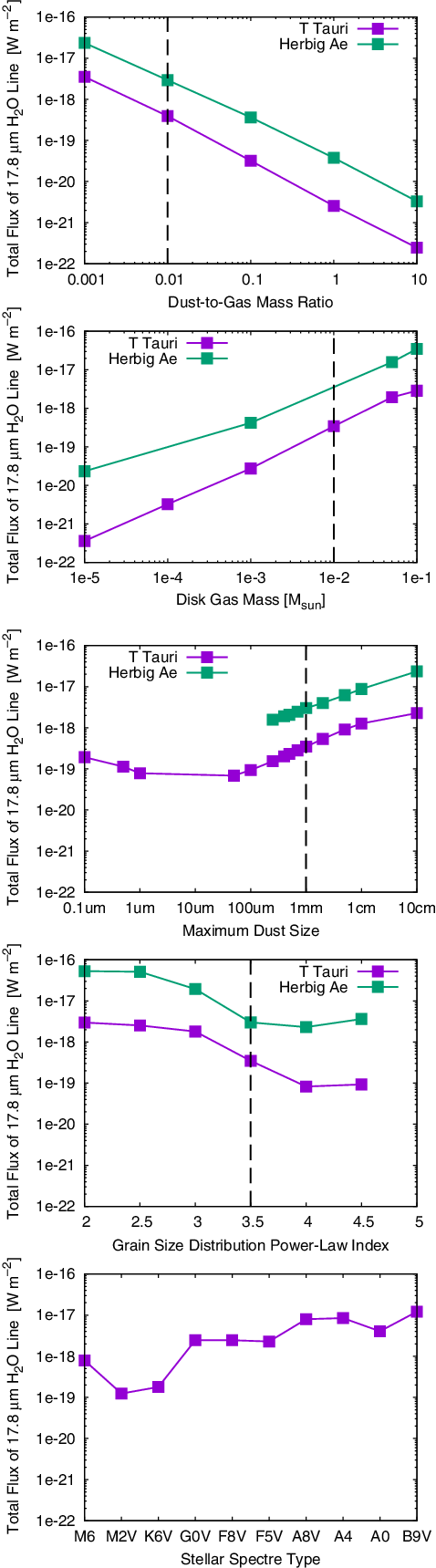
Figure 22. The 17.75-
 $\mu\mathrm{m}$
water line fluxes for various disk parameters around T Tauri and Herbig Ae stars. The dashed lines indicate the fiducial models (Antonellini et al. 2015; Reference Antonellini2016)
$\mu\mathrm{m}$
water line fluxes for various disk parameters around T Tauri and Herbig Ae stars. The dashed lines indicate the fiducial models (Antonellini et al. 2015; Reference Antonellini2016)
Our model calculations show that the line strength of the 17.75-
 $\mu\mathrm{m}$
water emission from inside the snowline of a fiducial T Tauri disk located at 300 pc (at Serpens) is
$\mu\mathrm{m}$
water emission from inside the snowline of a fiducial T Tauri disk located at 300 pc (at Serpens) is
 $\sim\!1\times 10^{-19}\,\mathrm{W\,m}^{-2}$
and that of a fiducial Herbig Ae disk located at 420 pc (at Orion A/B) is
$\sim\!1\times 10^{-19}\,\mathrm{W\,m}^{-2}$
and that of a fiducial Herbig Ae disk located at 420 pc (at Orion A/B) is
 $\sim\!1\times 10^{-18}\,\mathrm{W\,m}^{-2}$
after subtracting dust continuum emission (Figure 20). The flux and flux density sensitivities of SMI/HR are
$\sim\!1\times 10^{-18}\,\mathrm{W\,m}^{-2}$
after subtracting dust continuum emission (Figure 20). The flux and flux density sensitivities of SMI/HR are
 $\sim\!1\times 10^{-20}\,\mathrm{W\,m}^{-2}$
and
$\sim\!1\times 10^{-20}\,\mathrm{W\,m}^{-2}$
and
 $\sim\!1.4$
mJy, respectively, for 5
$\sim\!1.4$
mJy, respectively, for 5
 $\sigma$
in 1-h integration time. The synthetic analysis of the line profiles with spectral resolution of
$\sigma$
in 1-h integration time. The synthetic analysis of the line profiles with spectral resolution of
 $R=29,000$
and sampling of
$R=29,000$
and sampling of
 $N=1.5$
shows that the noise level is low enough so that the synthetic data can be fitted with a double peak profile within 1-h integration time for a T Tauri disk located at 300 pc (at Serpens) and within 10-min integration time for a Herbig Ae disk located at 420 pc (at Orion A/B) (Figure 21). Thus, in order to recover the water line profile (total line flux of
$N=1.5$
shows that the noise level is low enough so that the synthetic data can be fitted with a double peak profile within 1-h integration time for a T Tauri disk located at 300 pc (at Serpens) and within 10-min integration time for a Herbig Ae disk located at 420 pc (at Orion A/B) (Figure 21). Thus, in order to recover the water line profile (total line flux of
 $8.5\times 10^{-20}\,\mathrm{W\,m}^{-2}$
at 300 pc, FWHM
$8.5\times 10^{-20}\,\mathrm{W\,m}^{-2}$
at 300 pc, FWHM
 $\sim\!40-60\,\mathrm{km\ s}^{-1}$
, T Tauri disk), we need a noise level of 0.28 mJy for a continuum of 10 mJy. We then scale the noise level with the continuum using the 12-
$\sim\!40-60\,\mathrm{km\ s}^{-1}$
, T Tauri disk), we need a noise level of 0.28 mJy for a continuum of 10 mJy. We then scale the noise level with the continuum using the 12-
 $\mu\mathrm{m}$
fluxes from WISE.
$\mu\mathrm{m}$
fluxes from WISE.
Since the water line flux depends on the various parameters of the disks (Figure 22), the target objects will be selected more specifically based on the forthcoming JWST observations of water lines with lower spectral resolution and ALMA observations of CO lines for determining inclination angles of the disks.
We note that this snowline survey will also provide the data for the disk dispersal case (Section 3) since the water line is systematically weaker than the
 $\mathrm{H}_2$
and fine structure lines targeted there. Also, SMI/HR covers the wavelengths of various molecular lines which enable us to carry out additional science, such as measuring the C/O ratio in the inner disks using various mid-IR lines and measuring gas masses at the last stage of gas dispersal from the disks using
$\mathrm{H}_2$
and fine structure lines targeted there. Also, SMI/HR covers the wavelengths of various molecular lines which enable us to carry out additional science, such as measuring the C/O ratio in the inner disks using various mid-IR lines and measuring gas masses at the last stage of gas dispersal from the disks using
 $\mathrm{H}_2$
lines.
$\mathrm{H}_2$
lines.
A.4 Isolated Debris disks gas/Ice survey
The goal of this programme is to determine the composition of planetesimals in debris disks using a combination of gas line detections with SAFARI/HR to probe their volatile content that is released in collisions, and solid-state features with SAFARI/LR to probe the composition of the dust. While an observation of even a single-debris system would be significant, to answer the broader question of how the chemical make-up correlates with the stellar type and the presence of planets, and to ultimately link chemical composition to planet formation, a sample size on the order of 100 systems is desired. This will allow the sample to be divided by various properties to allow to search for trends. That is, it is not sufficient to simply derive a volatile content of a few disks, rather the aim is to make a predictive model that can be used to constrain protoplanetary disk evolution models and to determine how this composition affects the evolution of any planetary system including its habitability. Thus, it is important to ascertain how volatile content depends on planetesimal belt radius, stellar luminosity and age, or other properties of the planetary system. There are also several parameters that need to be constrained for the model to make accurate predictions, such as the level of viscosity in the gas disk and how that depends on ionisation. These will provide fundamental insights into the underlying physics that are not the focus of this science case, but again argue for a large sample for success.
The targets that are most amenable to such a study are already known, since the sample of nearby debris disks with detectable dust emission is relatively complete based on IRAS, Spitzer, and Herschel surveys. Thus, we first compiled a sample of 486 such disks from which the model in Kral et al. (Reference Kral, Matrà, Wyatt and Kennedy2017) was used to predict the gas line fluxes. These line fluxes were calculated for two assumptions: gas stemming from Solar System like comet/planetesimal composition, and gas from four times drier material. We also used SED modelling to predict the contribution of stellar and dust emission at the 44
 $\mu\mathrm{m}$
of the ice feature from which to assess its detectability.
$\mu\mathrm{m}$
of the ice feature from which to assess its detectability.
We propose a three-tier strategy (three samples consisting of different objects):
-
Sample A: Observe
 $\sim\!40$
disks in LR and HR to a depth such that [O I] and [C II] can be detected if planetesimals are four times drier than Solar System comets.
$\sim\!40$
disks in LR and HR to a depth such that [O I] and [C II] can be detected if planetesimals are four times drier than Solar System comets. -
Sample B: Observe
$\sim\!40$
disks in LR and HR to a depth such that [O I] and [C II] can be detected if planetesimals are similar to Solar System comets. -
Sample C: Observe
$\sim\!60$
disks in LR only to detect the water ice feature.


The motivation for this is that Sample A will say how dry planetesimals are typically and determine dependence on spectral type. Sample B will expand this to determine volatile dependence on planetesimal belt radius, age, presence of planets, etc. Sample C will use ice features as a proxy for volatile content (using relations calibrated with samples A and B) allowing us to probe parameter space not covered in the other samples due to the prohibitively long integration times that would be required to detect gas (later spectral types and lower fractional luminosity). This leads to a total sample of 80 objects (sample A and B) for which we request HR observations and a total sample of 140 targets (sample A, B, and C) for which we request LR observations. For the latter, we aim for a S/N ratio of 5 on the predicted photospheric continuum level.
We expect that the samples A and B will already have CO gas detections with ALMA within the next decade. On their own, these CO detections would not be able to make predictions for the volatile content of the planetesimals (in particular of water ice), but in combination with the SPICA gas lines such accurate predictions would be possible. There are already
 $\sim\!20$
debris disks with CO detected by ALMA, and the detection thresholds predicted by Kral et al. (Reference Kral, Matrà, Wyatt and Kennedy2017) imply that
$\sim\!20$
debris disks with CO detected by ALMA, and the detection thresholds predicted by Kral et al. (Reference Kral, Matrà, Wyatt and Kennedy2017) imply that
 $\sim\!100$
CO and [C I] detections can be expected with ALMA in the next decade, covering a similar sample to that proposed for SPICA observations of [C II] and [O I].
$\sim\!100$
CO and [C I] detections can be expected with ALMA in the next decade, covering a similar sample to that proposed for SPICA observations of [C II] and [O I].
The total integration time using the SAFARI estimator version 1.2 (issue 3.0; this version did not yet include the impact of the source background) is 54.5 h for sample A and B for the high-resolution spectra. In addition, we request 94 h for sample A, B, and C for the SAFARI/LR mode (version 1.2, issue 6.2).
This isolated debris disk sample complements the class III disks in SFRs from the HD survey. The isolated debris disks are typically much older than 100 Myr, while the class III disks in SFRs and MGs present the younger counterpart (1–100 Myr). For those, we target primarily the fainter HD lines, ensuring that the [O I]
 $63\,\mu\mathrm{m}$
and [C II] 158
$63\,\mu\mathrm{m}$
and [C II] 158
 $\mu\mathrm{m}$
for all targets will be detected.
$\mu\mathrm{m}$
for all targets will be detected.