


1. Introduction
Ever since Darwin’s ‘Origin of Species’ (Reference Darwin1859), the incompleteness of the fossil record has plagued our understanding of biodiversity through geological time. Major concerns focused on how to interpret biodiversity change, when raw patterns might be seriously distorted by uneven sampling effort and unequal outcrop availability (Raup, Reference Raup1972, Reference Raup1976a; Miller & Foote, Reference Miller and Foote1996; Smith, Reference Smith2007; Wall et al. Reference Wall, Ivany and Wilkinson2009; Mannion et al. Reference Mannion, Upchurch, Carrano and Barrett2011; Aberhan & Kiessling, Reference Aberhan, Kiessling and Talent2012). There are two prominent hypotheses explaining the covariation between rock quantity and biodiversity: rock record bias and common cause. The former proposes that diversity through time fully reflects rock availability, whilst the latter posits that the correlation between rock and fossil records is driven by a common cause, such as sea-level changes. Rock record bias may be profound, with some authors suggesting that it might account for more variation in sampled diversity than genuine fluctuations in biodiversity (Raup, Reference Raup1976b; Peters & Foote, Reference Peters and Foote2001; Smith et al. Reference Smith, Gale and Monks2001; Crampton et al. Reference Crampton, Beu, Cooper, Jones, Marshall and Maxwell2003; Peters, Reference Peters2006, Reference Peters2011; Smith, Reference Smith2007). However, both sedimentary rock and preserved biodiversity may be the results of a mutual response to environmental changes, such as long-term sea-level fluctuations (Peters, Reference Peters2008; Dunhill, Reference Dunhill2011; Hannisdal & Peters, Reference Hannisdal and Peters2011). Both hypotheses are not mutually exclusive, making it difficult to disentangle them.
Palaeontologists seek to reduce biases by means of sampling standardization (Alroy et al. Reference Alroy, Marshall, Bambach, Bezusko, Foote, Fursich, Hansen, Holland, Ivany, Jablonski, Jacobs, Jones, Kosnik, Lidgard, Low, Miller, Novack-Gottshall, Olszewski, Patzkowsky, Raup, Roy, Sepkoski, Sommers, Wagner and Webber2001; Alroy et al. Reference Alroy, Aberhan, Bottjer, Foote, Fürsich, Harries, Hendy, Holland, Ivany, Kiessling, Kosnik, Marshall, McGowan, Miller, Olszewski, Patzkowsky, Peters, Villier, Wagner, Bonuso, Borkow, Brenneis, Clapham, Fall, Ferguson, Hanson, Krug, Layou, Leckey, Nürnberg, Powers, Sessa, Simpson, Tomašových and Visaggi2008; Alroy, Reference Alroy2010; Close et al. Reference Close, Evers, Alroy and Butler2018), the basic idea of which is to draw a certain number of items (taxonomic lists and fossil occurrences) or acquire equal coverage of a rank abundance distribution from a dataset to standardize for sampling intensity across time and space. Subsampling has become a popular method to reveal sampling-standardized diversity trends, for example, with fossil occurrence data in the Paleobiology Database (PBDB; https://paleobiodb.org) (Alroy et al. Reference Alroy, Aberhan, Bottjer, Foote, Fürsich, Harries, Hendy, Holland, Ivany, Kiessling, Kosnik, Marshall, McGowan, Miller, Olszewski, Patzkowsky, Peters, Villier, Wagner, Bonuso, Borkow, Brenneis, Clapham, Fall, Ferguson, Hanson, Krug, Layou, Leckey, Nürnberg, Powers, Sessa, Simpson, Tomašových and Visaggi2008, Alroy, Reference Alroy2010). The PBDB is a global inventory of fossil occurrences in their geological and stratigraphical context. Although subsampling can mitigate the effect of collection biases on the Phanerozoic diversity curve (Alroy et al. Reference Alroy, Aberhan, Bottjer, Foote, Fürsich, Harries, Hendy, Holland, Ivany, Kiessling, Kosnik, Marshall, McGowan, Miller, Olszewski, Patzkowsky, Peters, Villier, Wagner, Bonuso, Borkow, Brenneis, Clapham, Fall, Ferguson, Hanson, Krug, Layou, Leckey, Nürnberg, Powers, Sessa, Simpson, Tomašových and Visaggi2008), a major pitfall is that unfossiliferous strata are not considered in the PBDB. Unfossiliferous strata represent sampled rock units that are devoid of fossil remains. Without such true absences of fossils being reported (e.g. a sampled but unfossiliferous sedimentary stratum), we cannot distinguish between a genuine lack of fossils and the absence of rock material (Peters, Reference Peters2007). Only the record of true absences will therefore allow an accurate interpretation of the correlation between rock volume and biodiversity and may help us unravel the relative importance of rock bias and common cause in explaining large-scale variations in sampled diversity.
The Geobiodiversity Database (GBDB; https://www.geobiodiversity.com) fulfils the requirement of recording genuine fossil absences from sedimentary strata. The GBDB is a vessel for stratigraphic columns, representing measured sections and providing rock units and fossil collections with geological context (Fan et al. Reference Fan, Chen, Hou, Miller, Melchin, Shen, Wu, Goldman, Mitchell, Yang, Zhang, Zhan, Wang, Leng, Zhang and Zhang2013), be they with or without fossil remains. Here, we use the macro-stratigraphical and palaeontological data from the GBDB to derive patterns of both genus diversity and rock quantity through the whole Phanerozoic. Each fossil collection is traceable and corresponding to a specific rock unit (Fig. S1). We address three questions: (1) Which geological proxies are most representative of palaeobiodiversity? (2) How strong is the rock quantity bias? (3) and To what extent do non-fossiliferous strata affect our estimation and interpretation of biodiversity in deep time?
2. Materials and methods
2.a. Data
As of May 2023, the GBDB comprised 217,969 geological units and 580,049 fossil occurrences ranging from the Ediacaran to the Quaternary. The GBDB is section-based providing bed-by-bed lithology information alongside their fossil content or lack thereof (Fig. S1). In this way, the GBDB has commonalities with the Macrostrat database (Peters, Reference Peters2006), which documents the macrostratigraphy of North America and the Caribbean. The GBDB can thus be viewed as a combination of the Paleobiology and the Macrostrat databases. That all lithological units in the GBDB are documented in terms of thickness also allows us to assess rock quantity in various ways, particularly in three dimensions instead of just the map-area approach used in earlier studies (Crampton et al. Reference Crampton, Beu, Cooper, Jones, Marshall and Maxwell2003; Smith & McGowan, Reference Smith and McGowan2007; Wall et al. Reference Wall, Ivany and Wilkinson2009).
The GBDB has been openly accessible since 2019, after a major overhaul (Li et al. Reference Li, Na, Chen and Zhu2021). The geochronological ages in the GBDB are retrieved from the age information of geological formation in the PBDB. In this way, roughly 1/3 of the stratigraphic units in the GBDB can be assigned to a geochronological time range. Potential homonyms were checked manually for geological formations. For example, the Miaogou Formation could be either Silurian or Cretaceous in age, and the Mural Formation occurs in the Cambrian (Skovsted et al. Reference Skovsted, Balthasar, Vinther and Sperling2021) and the Cretaceous Aptian/Albian (Madhavaraju et al. Reference Madhavaraju, González-León, Lee, Armstrong-Altrin and Reyes-Campero2010). Stratigraphically long-ranging formations and typos were also reviewed manually and corrected accordingly in the GBDB. All GBDB data are freely accessible at https://www.geobiodiversity.com/download/main, including fossil occurrences, fossil collections and geological units. Each occurrence is linked to its geological section via a unique unit id.
Lithologically, the GBDB distinguishes carbonates, siliciclastics, evaporites, volcanics and metamorphics. For our analyses, we retain only sedimentary rocks (i.e. carbonates and siliciclastics). To parse the dataset into marine and non-marine, we checked/revised every single geological formation according to environmental information provided in the PBDB or related publications. The environmental assignments were subsequently added to the GBDB. In the final dataset, 86% of occurrences are from China (Table S1). The Palaeozoic data are nearly all marine, whereas the post-Triassic data are a blend of terrestrial and marine sedimentary rocks.
Taxonomically, the dataset contains various fossil groups, including protists, animals and plants. Among animals, conodonts are the most abundant, followed by graptolites, brachiopods, trilobites, bivalves, corals, and other invertebrates and vertebrates (Table S2). Plants only account for ∼6% of all occurrences.
There are 1142 valid formations that could be constrained stratigraphically, with 516 formations assigned to a single stage. Of all formations, 852 formations can be recognized as marine sediments, whereas 290 formations are terrestrial or freshwater. Finally, 40,742 fossil collections and 71,130 sedimentary units could be assigned to a time range according to the stage-level subdivision of Geologic Time Scale 2020 (Gradstein et al. Reference Gradstein, Ogg, Schmitz and Ogg2020). The studied interval spans from the Cambrian to the Neogene with 90 stage-level bins. The collections comprise 226,219 occurrences of 11,147 genera. All analyses were conducted in R programming environment (R Core Team, 2022). The R scripts are available as supplementary online material (https://doi.org/10.5281/zenodo.10122452).
2.b. Measuring rock quantity
In this study, we employ three proxies to assess rock quantity: number of formations, sedimentary area and sedimentary volume per geological stage. Counting formations is straightforward. We tabulate the number of formations per stage, including the formations that are confined to the interval as well as those that cross the interval’s top and/or bottom boundary. We calibrate areal extents of sedimentary rock by the area of a polygon outlined by the known coordinates of a formation, which occurs at least at three different locations for any given time interval. We use the ‘spatstat’ R package (Baddeley & Turner, Reference Baddeley and Turner2005) to find a convex hull for a set of observed outcrop points for each formation. The area of the convex hull is then computed with the ‘geosphere’ package (Hijmans et al. Reference Hijmans, Karney, Williams and Vennes2021). The total area for each time interval is estimated by summing up the area of all formation polygons of that age. Sedimentary volume is the area multiplied by mean thickness of sampled formations for each time interval. Normally, formations have a scattered coverage resulting from non-deposition or uplift and erosion. Therefore, our estimates of rock area and rock volume may overestimate the real values. We use the standard deviation of a rock proxy’s log returns to measure volatility of the time series (Kiessling, Reference Kiessling2006).
2.c. Raw genus diversity
We assume that a genus or lithological unit is present throughout the whole time that its formation spans. This kind of range interpolation for both fossil and rock counting will obviously overestimate turnover at the boundaries of time bins. The variation in the length of formations’ stratigraphical duration may also cause multiple counts of single genus occurrences. To test these assumptions, the analyses are repeated removing the formations that span longer than one, two and three geological stages, respectively.
2.d. Testing sampling bias and rock bias
Here, we distinguish rock bias from sampling (collecting) bias. Sampling bias refers to the dependence of fossil diversity on the number of fossil collections. Rock bias refers to the effects of variation in sedimentary rock (unit, formation, area and volume) on changes of diversity. We also distinguish sedimentary rock with fossils from those without fossils to see whether rock quantity bias can only be accounted for when non-fossiliferous strata are considered. The number of sedimentary units, with fossils or not, is supposed to be a better sampling metric to represent a closer approximation of total sampling effort (e.g. collecting effort and rock availability) than any of other metrics alone (e.g. fossil collections and geological formations).
We use linear regression to measure how preserved biodiversity is affected by the sampling and rock bias. Because all variables are autocorrelated, we conduct analyses on generalized differences (g) to assess how changes in one biodiversity are influenced by changes in the other variable(s). Generalized differencing uses the actual autocorrelation coefficient of a time series to correct values instead of assuming an autocorrelation coefficient of one as is the case with first differences (McKinney & Oyen, Reference McKinney and Oyen1989; Kiessling, Reference Kiessling2005). Cross-correlation tests are conducted to check for temporal lags.
To separate the effects of variation in diversity deriving from rock quantity and to further test which proxy is most representative of rock quantity bias, we apply multiple regression models followed by model selection. Regression models treat genus richness (D) as the dependent variable and potential geological drivers as independent variables. Model selection using Akaike’s Information Criterion (AIC) is a method to find the ‘best’ statistical model in the sense that most variation of the dependent variable is explained with as few parameters as possible (Burnham & Anderson, Reference Burnham and Anderson2002). In our study, we seek to identify rock proxies associated with genus diversity over geological timescales. Apart from individual variables, two-way interactions are selected based on the following assumptions: (1) the effect of the number of formations (NF) on generic diversity (D) will depend on how many sedimentary units a formation can be divided into (the total number of sedimentary units, NU); (2) the effects of sampling probability of rocks on generic diversity will depend on the amount of non-fossiliferous strata (Nufu); and (3) sedimentary area (SA) and sedimentary volume (SV) contain significant information on generic diversity through horizontal and vertical distribution of formations. Accordingly, our most complex model is: gD ∼ gNU + gNF + gSA + gSV + gNufu + gNF : gNU + gNF : gNufu + gNF : gSA + gNF : gSV. This model is exposed to backward model selection. Coefficients (β, the number before each variable in a best model) are used to describe the strength of effect of each independent variable on diversity. To better understand the fitted model, we use the ‘visreg’ package (Breheny & Burchett, Reference Breheny and Burchett2017) to visualize the relationships between estimated variables as well as pairwise interactions.
2.e. Normalized diversities and sedimentary occupancy of fossils
To remove the sampling bias created by the variation in the quantity of sedimentary rocks, we statistically compare the observed Phanerozoic diversity with predicted diversity that is estimated by the best-fit regression model (similar to Smith & McGowan, Reference Smith and McGowan2007). The residuals of this regression equal all unmeasured parameters and may largely reflect the genuine biological signals that are not generated by variation in rock record. To test the extent to which the variation in sedimentary rocks affect diversity over time, we again use the time series of generalized differences of sampled diversity and rock record model.
To evaluate the effects of true absences (non-fossiliferous strata) on the estimation of biodiversity, we also measure sedimentary occupancy (rock coverage) by the proportion of fossil-bearing units in overall sedimentary units (FO). This is a metric of how fossiliferous rocks are distributed temporally and spatially.
3. Results
The patterns of raw genus richness and the amount of sedimentary rock are strikingly similar (Figure 1). A few main features that stand out from the raw diversity curve are the early Cambrian radiation, the Ordovician biodiversification, the protracted diversity declines in the middle Devonian, and the end-Permian extinction. However, these features are likely partially generated by sampling bias from the heterogeneous collecting effort and rock record. High correlation coefficients (R > 0.5) are found between raw genus diversity (gD) and all explanatory variables: number of fossil collections, number of sedimentary units (with fossils or not), number of formations, sedimentary area and volume (Figure 2). Among all predictors, sedimentary volume is the weakest. When diversity is compared with the number of sedimentary units devoid of preserved fossil record, it still shows a strong correlation (Figure 2c). This implies that observed diversity at any given time is strongly influenced by the chance of sampling true absences of fossils (unfossiliferous strata). The number of unfossiliferous strata does not introduce a fossil-dependent sampling bias but simply covaries with sampling effort. Time series of SA/SV show greater volatility than time series of other variables (Table 1), probably as a result of the greater estimation uncertainty. We also find that there are no temporal lags in the relationship between diversity and either sampling or rock record proxies (Figure 3). Our results on fossil–rock relationships remain robust when removing through-ranging formations (Fig. S2).

Figure 1. Genus diversity and its potential drivers across the Phanerozoic in the Geobiodiversity Database. D, raw genus diversity (sampled-in-bin). NC, number of collections. NF, number of formations. NU, number of sedimentary units. Nufu, number of sedimentary units without fossil records. SA, sedimentary area. SV, sedimentary volume. Ma, millions of years ago. Cm, Cambrian; O, Ordovician; S, Silurian; D, Devonian; C, Carboniferous; P, Permian; Tr, Triassic; J, Jurassic; K, Cretaceous; Pg, Paleogene; Ng, Neogene.

Figure 2. Binary relationships between raw genus diversity and explanatory variables. Linear regression lines are based on Pearson’s moment-product correlation: g, generalized difference. D, raw genus diversity. NC, number of collections. NF, number of formations. NU, number of all sedimentary units. Nufu, number of sedimentary units without fossil records. SA, sedimentary area. SV, sedimentary volume. All p-values are <0.001.
Table 1. Volatility of time series of all independent variables. NC, number of collections. NF, number of formations. NU, number of sedimentary units. Nufu, number of sedimentary units without fossil records. SA, sedimentary area. SV, sedimentary volume


Figure 3. Cross-correlation tests to compare pairwise relationships between diversity and rock quantity. All variables are generalized differences. All the best correlations occur at 0 lag, meaning that there is no temporal lag to the effect that the changes in rock record have the changes in diversity.
Model selection suggests that the best model for predicting diversity from the rock record is: gD ∼ 42.79 + 0.33·gNU + 3.43·gNF + 0.004·gSA – 0.04·gSV – 0.3·gNufu – 0.001·gNF : gSA + 0.005·gNF : gSV (adjusted R2 = 0.85, p < 0.001; Table 2). Any other variable removed from this model has a higher AIC and also less explanatory power (Table 2). To compare the relative importance of independent variables in this model, we standardized all variables to a mean of 0 and variance of 1. The best model after scaling is gD ∼ 0.002 + 1.56·gNU + 0.20·gNF – 0.04·gSA + 0.02·gSV – 0.79·gNufu – 0.14·gNF : gSA + 0.13·gNF : gSV (adjusted R2 = 0.85, p < 0.001). In this model, gNU has the largest influence on sampled diversity, suggesting that the number of sedimentary units have the greatest predictive effect on diversity among all variables. The visualization of the scaled regression (Figures 4, 5) shows that the number of unfossiliferous rocks (gNufu) negatively affects sampled diversity in this multivariate framework (Figure 4b). This is at odds with the strong positive correlation between gNufu and gD in the bivariate context (Figure 2c). Also in this multivariate framework, influences of rock area and rock volume on sampled diversity are minor (Figure 4d, e). When admitting that these two proxies slightly interact with geological formations (Figure 5), the positive effect of geological formations on sampled diversity is smaller when the depositional area becomes larger (see the changes in slopes in Figure 5a), whereas the dependence of genus diversity on the number of geological formations appears to become more pronounced with increasing volume of exposed rock outcrop (Figure 5b).
Table 2. Summary of multiple regression analyses with raw genus diversity as the dependent variable. Autocorrelations of dependent and independent variables were omitted with generalized differences (g). The lowest AICc indicates the best model. NF, number of formations. NU, number of sedimentary units. SA, sedimentary area. SV, sedimentary volume. Nufu, number of sedimentary units without fossil records


Figure 4. Partial residual plots to visualize the fitted model’s estimated relationship between generalized changes in each proxy of rock quantity and genus diversity. For each conditioning plot, the other variables are set to their median values. Shaded bands indicate 95% confidence intervals of the regression slopes. Note that the numbers of sedimentary units and unfossiliferous units align best with diversity.

Figure 5. Cross-sectional plots showing the estimated effects of two-way interactions on diversity in the fitted model. Left (a): The interaction between the number of formations (gNF) and sedimentary area (gSA). Right (b): The interaction between the number of formations (gNF) and sedimentary volume (SV). Each plot is partitioned into three linear regression models based on the 10th, 50th and 90th percentiles of the controlling variables on the top (Breheny and Burchett Reference Breheny and Burchett2017). Shaded bands indicate 95% confidence interval of the slopes. Note that the slope decreases with increasing gSA, suggesting that the effect of positive correlation between gNF and gD becomes smaller when sedimentary area is more extensive (the blue line shows a gentle slope in plane a), whereas the slope increases with increasing gSV, suggesting that the dependence of gD on gNF appears to become more pronounced with increasing sedimentary volume (the blue line shows the steepest slope in plane b).
When data are split into marine and terrestrial parts, the best models vary in terms of complexity and explanatory power (Table 3). In the Palaeozoic, nearly 93% of variability in diversity can be explained by the model with all selected variables in marine deposits. In the post-Palaeozoic, variation in the quantity of terrestrial sediments yields more explanatory power for genus diversity than that in marine sediments. The analysis also reveals that the negative predictive effect of unfossiliferous units on diversity is independent of marine and terrestrial deposits, with the strongest coefficient (β) in post-Palaeozoic marine sediments (Table 4), suggesting that decreasing diversity with increasing unfossiliferous units is not mainly driven by terrestrial sediments.
Table 3. Summary of best models based on model selection for marine and terrestrial sediments. NF, number of formations. NU, number of sedimentary units. SA, sedimentary area. SV, sedimentary volume. Nufu, number of sedimentary units without fossil records.

Table 4. Coefficients (β) of influence of unfossiliferous units (gNufu) in best models in predicting sampled diversity for marine and terrestrial sediments

With 85% of the variation in genus richness being attributable to rock record (Table 2), there is little room for genuine biological signals in our data. When removing the rock record bias from the detrended diversity curve, a biologically meaningful diversity time series might be revealed (Figure 6). The residuals do not show a clear trend through time, indicative of the correspondence between raw and predicted data. This suggests that peaks in sampled diversity are mainly the artefacts of an abundant rock record. The time series of fossil occupancy shows that in the Palaeozoic there is a nearly 50% (mean = 48 ± 2%) chance on average that a sampled sedimentary unit contains fossil remains, while this probability drops to about 20% (mean = 21 ± 1%) in the post-Palaeozoic (Figure. 7). This is mainly due to a shift towards terrestrial formations in the Late Triassic.
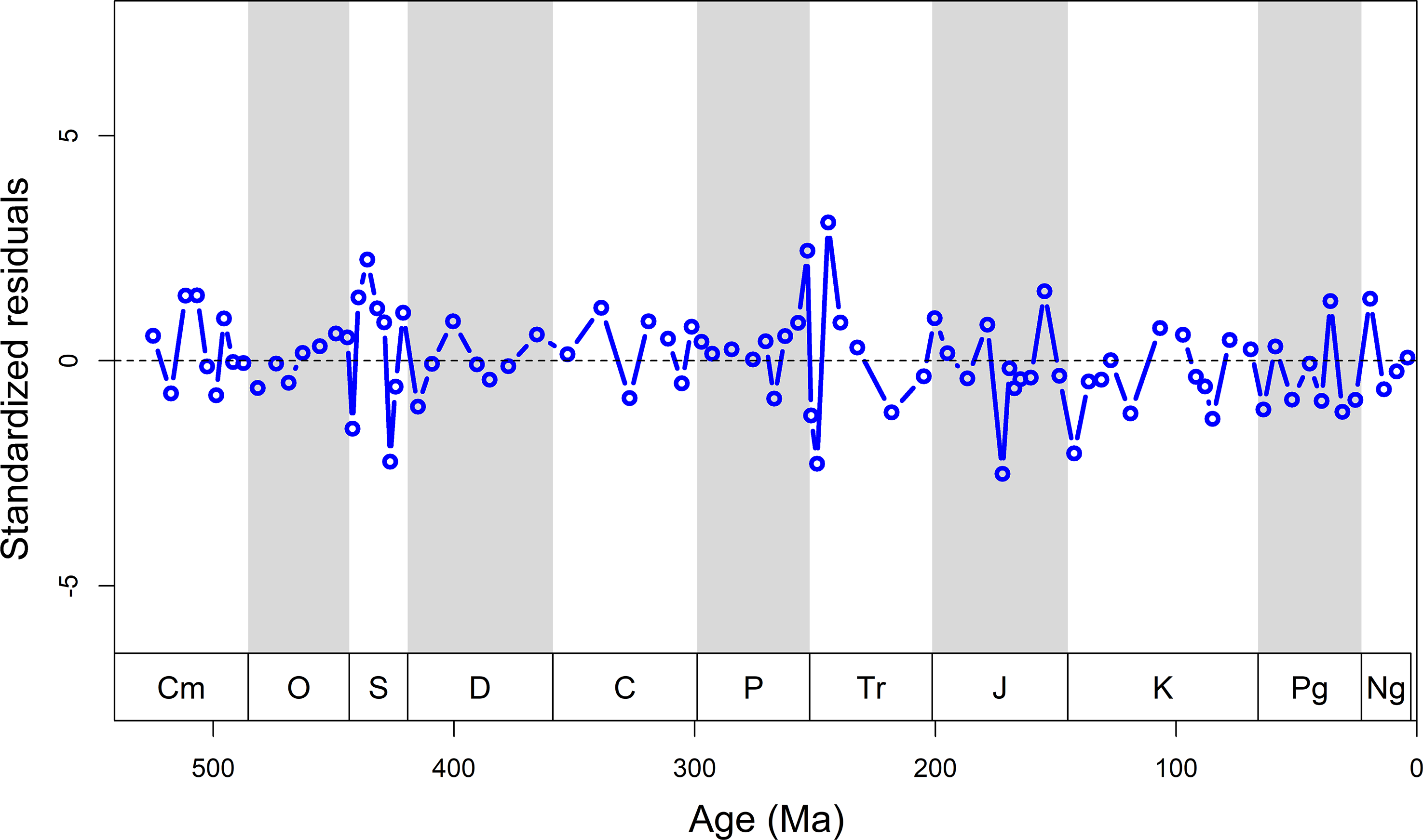
Figure 6. Standardized residuals remaining after removing the predicted diversity model curve from the observed diversity curve. Ma, millions of years ago.

Figure 7. Fossil occupancy through time. Black line denotes fossil occupancy (FO) in all sedimentary rocks measured by the proportion of fossil-bearing units. Grey line denotes the proportion of marine formations through time. Since Jurassic, terrestrial sediments became dominate in our dataset. Ma, millions of years ago.
Intervals with a poor rock record tend to produce artificially high extinction rates in the previous interval (Foote, Reference Foote2000; Peters & Foote, Reference Peters and Foote2002). Extinction rates should go up before the quality of the rock record declines, because ranges will be truncated when the fossil record declines (Foote, Reference Foote2000). However, we found no lagged cross-correlation between rock record and extinction (Figures 1, 8). Only one of the traditional Big Five mass extinctions depart significantly from the rock record model: the end-Permian mass extinction (Figure 8). The observed diversity in several time intervals, such as the Homerian (Silurian), Toarcian (Jurassic) and Berriasian (Cretaceous) stages, is also notably lower than the predicted diversity. These divergences occur when the rock record is poor or absent (Figure 1). Thus, it is hard to say if these deviations have any biological underpinning. Overall, for marine data observed and modelled diversities match almost perfectly (R2 = 0.90, p < 0.001). For the mixture of marine and terrestrial sediments in the post-Palaeozoic, the rock record cannot be solely responsible for recorded biodiversity (R2 = 0.55, p < 0.001).

Figure 8. Time series of generalized differences of observed diversity and predicted diversity derived from best-fit model. Asterisks mark time intervals where the drop in observed diversity is remarkably deviated from predicted from the rock record. Dashed lines denote five mass extinction events during the Phanerozoic. Ma, millions of years ago.
4. Discussion
At a global or continental scale, high sea-level increases the habitat area for marine benthic animals and thus marine diversity should increase at times when sea-level increases. Thus, long-term diversity trends may follow first-order global tectonic cycles of continental assembly and fragmentation (Fischer, Reference Fischer, Berggren and Van Couvering1984). However, the short-term fluctuations in observed diversity may mostly be attributed to rock availability and sampling effort (e.g. Peters, Reference Peters2005; Smith & McGowan, Reference Smith and McGowan2007). This is because at a local or regional scale, sea-level rise or transgression does not consistently increase the area of shallow marine habitat, nor does sea-level fall or regression always decrease shelf area (Holland, Reference Holland2012). Instead, the final exposure of rocks strongly depends on post-sedimentary modifications which are time-dependent (Raup, Reference Raup1976a) and is to some degree erratic (Benton et al. Reference Benton, Dunhill, Lloyd and Marx2011).
The number of collections and formations might be information-redundant with fossil richness reflecting bidirectional reinforcement of sampling bias and biodiversity (Dunhill et al. Reference Dunhill, Hannisdal and Benton2014bReference Dunhill, Benton, Twitchett and Newell). That is to say, greater sampling effort might result in higher fossil diversity, but more fossil finds might also in turn encourage more collecting. Recording only fossiliferous strata renders it impossible to identify sampling effort that failed to find fossils (e.g. Dunhill et al., Reference Dunhill, Benton, Twitchett and Newell2014aReference Dunhill, Benton, Twitchett and Newell; Maxwell et al. Reference Maxwell, Hopley, Upchurch and Soligo2018). In contrast, unfossiliferous sedimentary strata reflect a clear signal of sampling effort that is independent of the fossil record. In the bivariate context, both unfossiliferous strata and all strata are positively correlated with sampled diversity (Figures 2c, 3). Moreover, unfossiliferous strata are better correlated with the diversity of marine and terrestrial animals than sedimentary area and rock volume (Figures 4d, e). These results indicate that the rock bias mostly resulted from the genuine rock availability and is thus more relevant for recorded biodiversity than common-cause mechanisms such as sea-level changes that are mostly reflected in rock area/volume. Barren strata have been previously shown to be poorly correlated with maximum continental flooding (Smith and McGowan, Reference Smith and McGowan2008) rendering unfossiliferous strata not subject to the common cause. The impact of unfossiliferous strata on sampled diversity is still strong in terrestrial sediment where common cause should have little influence (Table 4).
As the largest part of our data is from China (Table S1), the dependency of diversity on the rock record may largely reflect the tectonic history of Chinese tectonic blocks over time. For example, the time series highlights when the rock record model is inconsistent with observed diversity during the mid-late Silurian (Figures 6, 8), which is likely the result of depositional hiatus in well-studied regions of Chinese blocks. The rarity of Silurian–Devonian data in the GBDB (Figure 1) is coincident with a depositional hiatus in several regions, which include (1) the unconformity between uppermost Middle–Upper Ordovician and the overlying upper Carboniferous in North China in the context of the Huaiyuan Orogeny (Zhen et al. Reference Zhen, Zhang, Wang and Percival2016), and (2) the Kwangsian Orogeny happened in South China and was interpreted as the key of the platform-wide hiatus ranges from the Wenlock (middle Silurian) to Carboniferous (Rong et al. Reference Rong, Chen, Su, Ni, Zhan, Chen, Landing and Johnson2003; Rong et al. Reference Rong, Wang, Zhan, Fan, Huang, Tang, Li, Zhang, Wu and Wang2018).
In addition, the occasional mismatch between the rock record model and diversity (Figure 8) may also reflect strong depositional bias caused by increasing records of terrestrial deposits towards younger ages (Figure 7). For example, the Jurassic and Cretaceous rocks in China were dominantly terrestrial with only a few marine facies scattered in the Qinghai-Tibet area, southern South China and northeast China (Huang, Reference Huang2019; Xi et al. Reference Xi, Wan, Li and Li2019). Due to higher abundance of terrestrial rocks, fossil occupancy is low in the strata of the Jurassic-Cretaceous (mostly lower than 0.2, Figure 7), suggesting that, compared to marine environments, fossil abundance in non-marine strata is generally low despite the famous Jehol Laterstätte of Cretaceous age (Zhou, Reference Zhou2014).
In sum, our analyses indicate that it is the change of depositional environments rather than biological crises, which contribute most to big shifts in biodiversity. Such environmental changes may explain the diversity drops at the end of the Silurian and in the post-Triassic. Earlier studies suggest that gap-bound sedimentary packages closely reflect the tectonically driven sea-level curve (Hannisdal & Peters, Reference Hannisdal and Peters2010), and thus, there should be a positive correlation between the number of formations and outcrop area/volume. But this positive relationship is not universal when the studied area suffered high tectonic activities (Crampton et al. Reference Crampton, Beu, Cooper, Jones, Marshall and Maxwell2003). One explanation could be that geographical distribution and thickness of sedimentary rocks are not homogeneous across time and space. Particularly, how thick a lithological unit can be is heavily dependent on rock facies and the subsidence rate of a basin (Smith & Benson, Reference Smith and Benson2013). Therefore, the recorded thickness of a sedimentary unit can vary from a few metres to hundreds of metres depending on depositional environment.
The accuracy and precision of the measure of rock availability are subject to uncertainty in stratigraphic binning. Correlations between sampling/rock proxies and palaeodiversity may get stronger as stratigraphic resolution becomes finer (Dunhill et al. Reference Dunhill, Benton, Twitchett and Newell2014aReference Dunhill, Benton, Twitchett and Newell). At stage level, the time series of NF and Nufu show less fluctuations than the time series of SA and SV (Table 1) suggesting that the quantity of geological formations and unfossiliferous strata are more geological meaningful. Convex-hull estimates of sedimentary area may overestimate true areas, but this will only affect our analyses if the overestimation is not consistent over time and thus represents a bias rather than a random error. Given that the GBDB data suffer from heterogenous research effort and the preservation is not consistently good (e.g. marine is better than terrestrial), the effect of rock area/volume on sampled diversity could be distorted. Further work needs to improve the accuracy of measuring rock availability to better compensate for sampling biases in long-term palaeodiversity curves.
5. Conclusions
Our multiple regression analysis suggests that the variation in a single rock proxy cannot account for the overall rise and fall in sampled diversity. Rather large-scale geological controls of sampled biodiversity correlate with all rock proxies, and there are substantial synergies among different proxies indicating that influences among rock-record proxies may play a crucial role in shaping preserved diversity, especially regarding the marine record. Most importantly, we find strong evidence for a covariation of unfossiliferous strata and genus richness, and we propose that this is best explained by research effort. Hence, rock record bias rather than common-cause mechanisms are held to be largely responsible for long-term variations in observed fossil biodiversity.
Supplementary material
To view supplementary material for this article, please visit https://doi.org/10.1017/S0016756823000742
Data availability
Data and code required to reproduce the results are accessible through Zenodo (https://doi.org/10.5281/zenodo.10122452)
Acknowledgements
We appreciate the helpful reviews of M. E. Clapham and one anonymous reviewer. We thank all the contributors to the Geobiodiversity and Paleobiology Databases. In particular, we thank J-X Fan, R-B Zhan, C. J. Reddin and S. E. Peters for their support and discussion. This work is funded by the State Key Laboratory of Palaeobiology and Stratigraphy (Nanjing Institute of Geology and Palaeontology, CAS) (20202103), and by the National Natural Science Foundation of China (42372039). This paper is contributed to IGCP 735 ‘Rocks and the Rise of Ordovician Life: Filling knowledge gaps in the Early Palaeozoic Biodiversification’ and Volkswagenstiftung project ‘Strengthening Paleontology: The German hub for global cooperation’. This is Geobiodiversity Database publication No. 1 since publication tracking in 2023 and Paleobiology Database publication No. 472.
Competing interests
The authors declare none.


 Open access