


Introduction
During September 1996 one of us (P.W.) took part in an Arctic operational voyage by HMS Trafalgar during which upward sonar profiling of the ice canopy was carried out, together with sidescan sonar profiling and along-track temperature, salinity and fluorescence monitoring. We here report on the ice-draft characteristics revealed by the upward-looking sonar, of which two systems were in simultaneous use. The first was an Admiralty-pattern 780 system, recording on paper chart; this was identical to the system used by HMS Superb in May 1987 (Reference WadhamsWadhams, 1992), and on other UK submarine voyages of the 1980s and early 1990s from which data have recently been released but not yet analyzed. The second was a new narrow-beam digital system, the 2077, which is better at resolving the structure of individual pressure-ridge keels. In a future paper we will report on comparisons between the two systems; in the present paper we report on results obtained from the 2077 only.
In October 1976 a voyage to the same part of the Arctic was carried out by HMS Sovereign, and similar datasets collected (Reference WadhamsWadhams, 1981). Since the seasons were almost identical, we compare results from the two cruises in order to test whether the thinning observed over a similar time lapse by Reference Rothrock, Yu and MaykutRothrock and others (1999) in other parts of the Arctic is applicable also to the region between Fram Strait and the North Pole.
Data Analysis
An advantage of the 2077 system is that it is coupled to the boat’s inertial navigation system, so that data are recorded directly as draft vs horizontal distance. This avoids one of the most time-consuming tasks with the 780 sonar, which is the need to combine the draft-time profile record with the boat’s navigation to yield a draft-distance relationship. In addition, the 2077 automatically removes submarine depth variations so as to yield a continuous sea-level profile which is subtracted from the measured range to the ice bottom so as to yield a draft. However, accurate depth removal was dependent upon knowing the vertical sound velocity profile between the boat and the sea surface. This profile, based on periodic XSV (expendable sound velocity) casts, could only be updated at intervals, and so an error in range, and hence in inferred draft, could develop. Fortunately, the summer ice cover was remarkably open, and contained many unfrozen leads (identified via the upward TV camera record and from the high sonic reflection coefficient of open water). These provided frequent zero references through which the zero error could be removed. Corrected drafts were then grouped in 50 km data lengths, and statistics were generated.
Figure 1 shows schematically the track of the submarine. The track within the Eurasian Basin north of Fram Strait comprised a "westerly" leg at about 5° Wand an "easterly" leg at about 5° E. These were analyzed separately to test for zonal variations in mean ice thickness. Within the Greenland Sea the track can again be divided into a westerly leg which followed the core of the East Greenland Current over the shelf break, sampling typical ice conditions for each latitude, and an easterly leg which lay more within the marginal ice zone (MIZ).

Fig. 1. Schematic diagram of submarine tracks, (a) september 1996, (b) october 1976.
Mean Ice Draft
The dataset with which the 1996 profiles are compared was obtained in September-October 1976 by HMS Sovereign (Reference WadhamsWadhams, 1981). Figure lb shows Sovereign’s track alongside that of Trafalgar. Sovereign was equipped with a sonar system which had a narrow beamwidth in the athwartships direction but a wider beam fore-and-aft. A correction for beamwidth effects was applied to the data (Reference WadhamsWadhams, 1981) by applying a calibration based on convolving a genuinely narrow-beam ice profile (that of USS Gurnard, 1976) with a sonar beam of width equal to that aboard Sovereign, then examining the percentage change in mean draft occurring in different ice regimes. We can therefore legitimately compare the Sovereign data (beam-width-corrected) with the Trafalgar data (not beamwidth-corrected, but obtained by a narrow-beam instrument).
The protocol of track selection was to compare those portions of the tracks of the two submarines which lay in 1 ° latitude increments and within the longitude limits 5° W to 5° E. This involved a total of about 2100 km of track from each submarine, and corresponds as closely as possible to Reference Rothrock, Yu and MaykutRothrock and others’ (1999) concept of "crossing tracks". The resulting mean ice drafts are as shown in Table 1.
Table 1. Mean ice drafts 1˚ latitude bins spanning greenwich meridian from september 1996 Trafalgar cruise and september-october 1976 Sovereign cruise

The overall decline in mean ice draft between 1976 and 1996, giving equal weight to each latitude range between 81 ° N and 90° N, is 43.2%, which is close to the value found by Reference Rothrock, Yu and MaykutRothrock and others (1999) for the Arctic basin as a whole. We note that Rothrock and others’ track comparisons occur over the North Pole region and Canada Basin, with few in the Eurasian Arctic and none south of 84° N in the Eurasian Basin. These results therefore both support the U.S. findings and extend them to a part of the Arctic not covered by U. S. datasets.
There was a seasonal displacement of, on average, 4 weeks between the 1976 and 1996 experiments. Reference Rothrock, Yu and MaykutRothrock and others (1999) "standardized" their datasets, obtained during various periods of the summer between July and October, to 15 September by the use of a sea-ice model. If we tentatively use the same seasonal cycle as shown in Reference Rothrock, Yu and MaykutRothrock and others (1999), a small seasonality correction gives us a decline of 41 % rather than 43.2%, still in good agreement with the U.S. results.
Ice-Draft Distributions
Figure 2 shows four examples of histograms of the draft distribution of the westerly track of the 1996 cruise, plotted to a maximum draft of 10 m. In each case a characteristic of the distributions is the large fraction of open water and thin ice (first band in histogram; <10 cm deep), even in the 89−90° N example. The Greenland Sea histogram consists mainly of thin ice, with a low mean draft (Table 2) and no peak characteristic of typical Arctic first- or multi-year thicknesses. The Fram Strait example also contains much young ice, but there is a peak at 2.5 m draft which is typical of melting multi-year ice. The examples within the Eurasian Basin show a peak at about 2.5 m, together with increasing amounts of deeper, ridged ice. However, as compared to earlier thickness distributions from the late-summer or autumn period (e.g. HMS sovereign data from October 1976, shown in Reference WadhamsWadhams, 1981), these distributions show very much reduced amounts of thicker ice. The mean ice drafts in Table 2 differ slightly from those in Table 1, which contains only those track sections which lay between 5° Wand 5° E.

Fig. 2. Probability density functions of ice draft from four regions of the 1996 cruise.
Table 2. Statistical parameters derived from data in 1° latitude bins, 1996 cruise
The 1° binned ice-draft distributions are shown plotted against latitude for both tracks (Fig. 3) where the data are displayed for total, level and rough ice, and the decline in open water/thin ice with increasing latitude is clearly illustrated. Level ice is defined by a simple slope criterion. In both cases the continuing high incidence of open water and very thin ice at all latitudes is apparent, while the level-ice plots (particularly the easterly track) show a radical drop in the draft of the main peak south of Fram Strait (80° N), indicating rapid melt within the Greenland Sea. The rough-ice plots show a similar transition at about the same latitude, with the thick ice in the 5−10 m draft range almost disappearing.

Fig. 3. Probability density functions of 1996ice draft in 1˚ bins plotted against latitude for westery and easterly tracks. top: all ice; middle: level ice only; bottom: rough ice only.
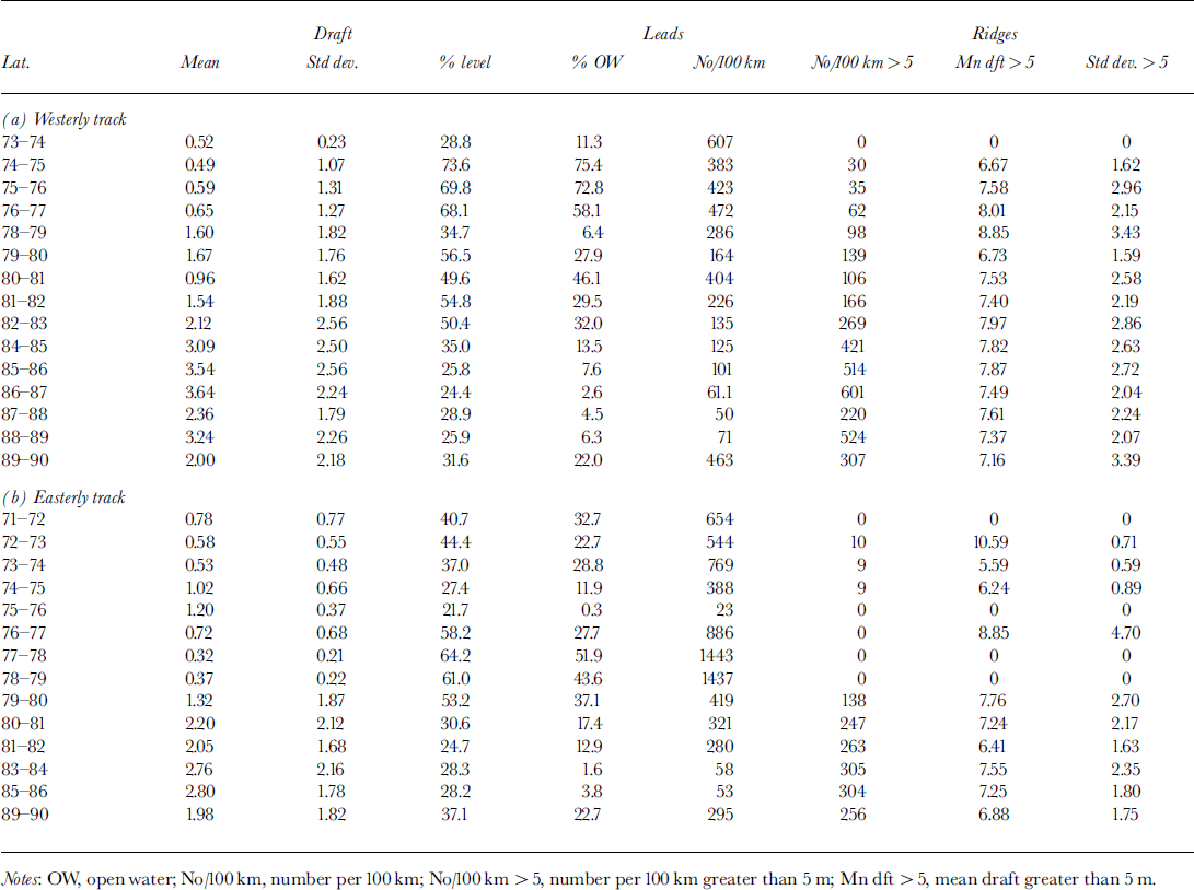
Pressure Ridges and Leads
Table 2 shows statistics for pressure-ridge and lead occurrences for the westerly and easterly tracks in 1° bins. A missing bin implies that <50km of track data were available within that degree increment. Independent ridges were defined in the same way as for previous analyses (Reference WadhamsWadhams, 1981, Reference Wadhams1992), with a minimum draft value of 5 m. Leads were defined as features at least 5 m wide containing ice of draft <30cm. It can be seen that there is a radical drop in ridge frequency south of Fram Strait, while lead occurrence is more variable. The ridging variation can be seen more clearly by considering the volume of ridged ice per unit length of track. This should be proportional to nh2, where n is the number of ridges per unit track length and h is the mean draft, on the assumption that ridges of all depths have the same average shape factor (ratio of cross-sectional area to square of draft).
Figure 4 (drawn from westerly track data) shows that, with track length expressed in km and ridge draft in m, the relative volume increases from 13 at 74° N to 130−340 in the zone north of Fram Strait. The most rapid change occurs within and just north of the Strait, in the region 80−82° N. The percentage of surface occupied by leads ranges from 72−75% in the lower latitudes, to 28−46% within Fram Strait and lower values of < 10% near the Pole, with an increase to 22% at the Pole itself. The large variability is a statistical one, due to the open water and young ice being contained within a limited number of leads; the question of the statistical variability of parameters extracted from finite lengths of track has been examined by Reference WadhamsWadhams (1997), who found that open-water fraction has a much higher variability than ridge frequencies.

Fig. 4. Percentage of open water, and relative volume of ridged ice (expressed as nh2 , where n is number of ridges per km, and h is ridge draft in m), as functions of latitude.
Parameter Relationships
Relationships between statistical quantities were explored, to investigate likely interactions which might allow the ice morphology to be parameterized, or related to quantities detectable by satellite. The percentage of open water, a quantity that can be derived from passive-microwave or observed from visible-band sensors, was, as expected, negatively correlated with mean draft (Fig. 5). Reference Davis and WadhamsDavis and Wadhams (1995) found that the frequency of pressure ridges was lower in ice regimes with large amounts of open water, and this was also observed here (Fig. 6). The fraction of rough ice, which is mainly ice that has undergone deformation processes (although some undeformed multi-year ice might be rough enough to be counted), might also be expected to be related to the occurrence of pressure ridges, and this is also repeated here (Fig. 7). The other strongly suggested relationship is shown when correlating pressure-ridge occurrence with the overall mean ice draft (Fig. 8). Note that the relationship becomes less strong with high mean ice drafts.

Fig. 5. Mean draft of a 50 km section of track plotted against percentage open water in the section.

Fig. 6. Percentage open water plotted against number of ridges per km, in 50 km track sections.

Fig. 7. Percentage of rough ice in a 50 km section plotted against number of pressure ridges deeper than 5 m per km of track.

Fig. 8. Mean draft of a 50 km section plotted against number of pressure ridges deeper than 5 m per km of track.
Depletion of Thick Ice and Deep Ridges
The statistics presented so far indicate clearly that the ice cover in 1996 was very open, with much thin ice and open water present, and with a relative absence of very thick ice. A comparison with the 1976 sovereign data enables us to see more clearly the magnitude of the thick-ice depletion. The first question that we can answer is, to what extent can the decline in mean ice thickness shown in Table 1 be ascribed purely to the more open nature of the ice cover? If all the ice not in leads were pushed up together, would the mean thickness still be less? The answer is resoundingly positive. Figure 9 shows the results of calculating the mean thickness of all ice thicker than 0.5 m for 1976 (100 km sections in the range 10° W to 10° E) and 1996 (1 ° sections from easterly and westerly tracks) using data from north of 78° N. There is still a very substantial decline in mean thickness in 1996.

Fig. 9. Mean drafts for ice deeper than 0.5 m from 1976 and 1996 data, between 78° n and north pole in region 10° w to 10° e.
The second question is, what contribution to the thinning is made by a loss of very thick ice? Very thick ice is all contained in pressure ridges, so we can examine the comparative statistics for all pressure ridges deeper than 9 m for 1976 and 1996. Figure 10 shows a plot of ridge numbers per km of track against mean ridge draft for ridges deeper than 9 m found in 1976 and 1996 (data north of 81° N as for Fig. 9). The loss of pressure ridges is startling. There is no overlap between the envelope of the 1976 and 1996 results, i.e. there is no part of the region where there was as much ridging in 1996 as in 1976. On average, in this region of the Arctic, there were only a quarter as many deep ridges in 1996 as in 1976. It is clear that one of the most important aspects of the Arctic ice cover in its newly reduced state is that deep pressure ridges are now almost absent.

Fig. 10. Ridges deeper than 9 m: a plot of mean keel draft against mean number of ridges per km for data from 1976 and 1996 between 81° n and the north pole.
Conclusions
This cruise has provided a contemporary snapshot view of summer ice conditions in the Eurasian Basin and Greenland Sea. A remarkable loss of ice thickness is observed relative to older summer data. As compared to data from the sovereign cruise of October 1976, the mean thickness over the latitude range 81−90° N is reduced by 43%, in agreement with summer data from other parts of the Arctic basin reported by Reference Rothrock, Yu and MaykutRothrock and others (1999). The thinning reveals itself through larger amounts of open water, a low mean draft of undeformed ice and a shortage of deep pressure ridges. Of these changes, the significant decline in the occurrence of pressure ridges represents a major change in the morphology of Arctic sea ice.
Acknowledgements
We are grateful to the U.K. Ministry of Defence (Navy) for the release of data; to Flag Officer Submarines for the opportunity to take part in the voyages concerned; to the Commanding Officer and crew of HMS trafalgar, and for financial support to the U. K. Natural Environment Research Council and the U.S. National Science Foundation.


