


1. Introduction
The inviscid instability mechanism dominating laminar-turbulent transition of swept wing boundary layers (BL) in the region of a favourable pressure gradient is the so-called crossflow instability (CFI) (Mack Reference Mack1984; Arnal & Casalis Reference Arnal and Casalis2000; Saric, Reed & White Reference Saric, Reed and White2003). Primary stationary instabilities induce a spanwise momentum modulation, distorting the boundary layer and introducing strong spanwise and wall-normal velocity shears. These are highly susceptible to secondary instability mechanisms of a Kelvin–Helmholtz nature (Malik et al. Reference Malik, Li, Choudari and Chang1999; Wassermann & Kloker Reference Wassermann and Kloker2002; Bonfigli & Kloker Reference Bonfigli and Kloker2007; Serpieri & Kotsonis Reference Serpieri and Kotsonis2016), which undergo explosive growth ultimately leading to turbulence transition.
One of the most challenging aspects of CFI investigations is the characterization of the receptivity process (Morkovin Reference Morkovin1969). Early experiments outline the strong sensitivity of both stationary and travelling CFI to surface roughness and free-stream turbulence (Bippes Reference Bippes1999; Radeztsky, Reibert & Saric Reference Radeztsky, Reibert and Saric1999; Kurian, Fransson & Alfredsson Reference Kurian, Fransson and Alfredsson2011). In particular, in low turbulence environments, such as free flight ( $T_u/U_{\infty }<0.15\,\%$), stationary crossflow vortices are found to dominate BL stability and transition. Moreover, one of the relevant flow features resulting from receptivity is mode selection, which for stationary CFI mostly depends on the wing surface roughness (Bippes Reference Bippes1999; White et al. Reference White, Saric, Gladden and Gabet2001; Downs & White Reference Downs and White2013). Stationary crossflow vortices manifest on the wing surface as a set of streaky structures almost aligned with the free-stream velocity, which ultimately lead to transition through a jagged stationary front (Müller & Bippes Reference Müller and Bippes1989; Dagenhart & Saric Reference Dagenhart and Saric1999). To enhance the spanwise uniformity of the boundary layer and developing instabilities, many experimental and numerical works apply an artificial forcing in the form of discrete roughness elements (DRE), periodically distributed along the wing span in the vicinity of the leading edge (Reibert et al. Reference Reibert, Saric, Carrillo and Chapman1996; Saric, Carrillo & Reibert Reference Saric, Carrillo and Reibert1998; Serpieri & Kotsonis Reference Serpieri and Kotsonis2016). The inter-spacing (i.e. spanwise wavelength) and height of these elements are fundamental towards conditioning the instabilities wavelength and initial amplitude, although a predicting relation between the array geometry and CFI onset still has to be found.
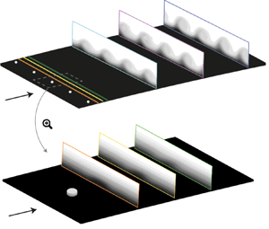
Despite the large body of experimental receptivity studies conducted to date, an estimation of the instability initial amplitudes ensuing from receptivity to  $T_u$ and roughness is still missing. To gain these insights, the investigation of the very initial phases of receptivity linked to the development of the near-DRE flow and the dominant flow structures is necessary, albeit extremely challenging. Due to the small scales of the flow phenomena involved, this flow region is hardly measurable experimentally. As an example, the measurements reported in the present work are performed on a swept wing model of more than 1 m chord and span developing a boundary layer with
  $\delta _{99} \simeq 1$ mm at 10 % of the chord, already downstream of the relevant receptivity region (Serpieri & Kotsonis Reference Serpieri and Kotsonis2015, Reference Serpieri and Kotsonis2016). Furthermore, the numerous parameters contributing to the receptivity process and their inter-dependencies along with the different flow scales involved complicate the development of numerical prediction tools. Of the many studies inspecting roughness receptivity of three-dimensional (3-D) BL, only few numerical simulations are dedicated to the roughness elements near-DRE flow features. Among these, Kurz & Kloker (Reference Kurz and Kloker2014, Reference Kurz and Kloker2015) outline a not linear dependence of the ensuing CFI amplitude on the roughness parameters, particularly height. The direct numerical simulations (DNS) by Kurz & Kloker (Reference Kurz and Kloker2016) details the roughness elements near-DRE flow features and their dominant instability mechanisms for both two- and three-dimensional BL. From their results, an overall similarity of the dominant near-DRE flow mechanisms is observed: in both cases a complex vortical system composed of two sets of horseshoe vortices develops around the element. Analogous near-DRE flow features for roughness elements in two-dimensional (2-D) BL are found in previous numerical works, such as Rizzetta & Visbal (Reference Rizzetta and Visbal2007), Denissen & White (Reference Denissen and White2008) and Doolittle, Drews & Goldstein (Reference Doolittle, Drews and Goldstein2014). An extensive analysis of the near-DRE flow stability is carried out by Loiseau et al. (Reference Loiseau, Robinet, Cherubini and Leriche2014), investigating a 2-D flat plate flow configuration experimentally measured by Fransson et al. (Reference Fransson, Brandt, Talamelli and Cossu2005). The work by Kurz & Kloker (Reference Kurz and Kloker2016) additionally characterizes the flow in the far-wake region, identifying significant differences between the 2-D and 3-D cases: in the former the flow evolves symmetrically aft of the element, while in the latter only the horseshoe legs co-rotating with the crossflow vortices are sustained, the others decaying shortly after. Their presence leads to a spanwise modulation of the velocity and momentum redistribution, hence, a low-speed hump forms immediately aft of the elements and fades downstream. The work by Kurz & Kloker (Reference Kurz and Kloker2016) represents a significant breakthrough in the investigation of near-DRE flow, although a clear relation allowing for the estimation of the initial amplitude of the ensuing CFI instabilities is not yet available.
A survey of past experimental and numerical works on receptivity of CFI reveals two unresolved challenges, which in turn have motivated and shaped the present work. The first is an incomplete understanding of the relation between roughness amplitude and location and the development of CFI and BL transition. Past work has focused either on global transition location correlations or localized measurements, typically using HWA under limited parameter ranges. Additionally, past studies made use of simplified metrics for the representation of the initial forcing amplitude such as height-based Reynolds number ( $Re_k$) or height to boundary layer thickness ratio. However, these metrics are often used only as an indication of supercritical behaviour (flow tripping), while it is still unclear whether they can correctly represent the initial forcing amplitude of DREs (Reibert et al. Reference Reibert, Saric, Carrillo and Chapman1996; Kurian et al. Reference Kurian, Fransson and Alfredsson2011; Kurz & Kloker Reference Kurz and Kloker2016). The present study aims at combining local and global transition and flow measurements, to better understand the main flow mechanisms dominating receptivity of stationary CFI to roughness arrays. Such a study aims also at establishing whether height-based metrics can be used to predict the initial forcing perturbation amplitude of a given roughness array configuration. Despite the minimal attention received throughout the literature, the location of the forcing arrays is one of the main parameters in this work, as it inherently governs the complex relationships between relative disturbances amplitude, local BL scales, pressure gradient and overall flow stability.
The second challenge is of a more practical nature and stems from the disparate scales governing the problem. More specifically, the detailed analysis of the evolving instabilities, in relation to amplitude and location of roughness elements conducted in this study, can provide effective scaling principles. Such scaling can give the possibility of reproducing the swept wing leading-edge flow features through an up-scaled forcing configuration more tractable in terms of experimental observability. In particular, the investigation of an up-scaled configuration would improve the experimental resolution of the near-DRE flow field, essential to clarify the relation between roughness and CFI onset, leading to a more complete understanding of receptivity and of the aforementioned conflicting outcomes in using DREs as a transition control technique.
2. Methodology
2.1. Wing model and wind tunnel facility
The presented measurements are performed in the low-speed low turbulence wind tunnel (LTT), an atmospheric closed loop tunnel located at the TU Delft. All acquisitions are performed at a chosen angle of attack  $\alpha =-3.36^\circ$ and Reynolds number
  $Re_{c_X}=2.17 \times 10^6$, computed in the free-stream direction. At these conditions,
  $T_u$ is sufficiently low (
 $T_u/U_{\infty } \simeq 0.025\,\%$, Serpieri Reference Serpieri2018) to let stationary crossflow waves dominate the stability and transition scenario (e.g. Bippes Reference Bippes1999; Downs & White Reference Downs and White2013).
The employed wind tunnel model is an in-house designed, constant-chord swept wing (M3J, table 1), extensively described in Serpieri & Kotsonis (Reference Serpieri and Kotsonis2015). The wing is purposely designed and widely used to investigate the physics of primary and secondary crossflow instabilities and laminar flow control techniques (e.g. Serpieri & Kotsonis Reference Serpieri and Kotsonis2016; Rius-Vidales et al. Reference Rius-Vidales, Kotsonis, Antunes and Cosin2018). This geometry features a favourable pressure gradient up to  $x/c\simeq 0.65$, figure 1(a), leading to the formation of a spanwise invariant boundary layer with laminar-to-turbulent transition process dominated by stationary crossflow instabilities. Due to the high sensitivity of CFI to surface roughness, the model surface is carefully polished ensuring a low and uniform roughness level (
 $R_q = 0.2\ \mathrm {\mu }{\rm m}$, Serpieri & Kotsonis Reference Serpieri and Kotsonis2015).
Table 1. Geometric parameters of M3J swept wing model (Serpieri & Kotsonis Reference Serpieri and Kotsonis2015).

Figure 1. (a) Plot of M3J airfoil geometry, averaged experimental pressure distribution and pressure gradient at  $\alpha = -3.36^{\circ }$,
  $Re_{c_X} = 2.17 \times 10^6$. (b) Plot of
  $N_{{eff}}$ curves for
  $\lambda _z=8\ {\rm mm}$ mode from LPSE solution initialized at different chordwise stations. Shaded regions describe
  $\lambda _z$ interval between 7 and 9 mm.
The model is equipped with two rows of chordwise distributed pressure taps which measure the pressure distribution on the wing pressure side. Two different coordinate reference systems can be defined for this wing model: one is integral to the wind tunnel floor, with spatial components given by  $X$,
$X$,  $Y$,
$Y$,  $Z$ and velocity components
  $U$,
$U$,  $V$,
$V$,  $W$; the second one has its z-axis aligned to the leading edge with spatial components
  $x$,
$x$,  $y$,
$y$,  $z$ and velocity u,
  $v$,
$v$,  $w$.
$w$.
2.2. Linear and nonlinear numerical stability simulation
The study of receptivity to roughness amplitude and location necessitates a prediction of the instabilities growth and initial amplitudes in regions of the boundary layer which are inaccessible to measurements. As such, the experimental measurements in this work are complemented by a stability simulation computed through an in-house developed routine (Westerbeek Reference Westerbeek2020) solving both linear and nonlinear parabolised stability equations (PSE, Bertolotti, Herbert & Spalart Reference Bertolotti, Herbert and Spalart1992; Simen Reference Simen1992; Hanifi, Schmid & Henningson Reference Hanifi, Schmid and Henningson1996; Herbert Reference Herbert1997). This approach has been widely applied to analyse the stability of 3-D BL developing on swept wings (Bertolotti Reference Bertolotti1996; Haynes & Reed Reference Haynes and Reed2000; Tempelmann et al. Reference Tempelmann, Schrader, Hanifi, Brandt and Henningson2012).
Stability solutions are computed for a reference base flow which is a steady and incompressible solution of the two-and-a-half-dimensional BL equations (based on spanwise invariance assumptions). The followed procedure, based on the experimentally acquired free-stream flow characteristics and pressure distribution, is fully described in Serpieri (Reference Serpieri2018).
The linear parabolized stability equations (LPSE) analysis is used to facilitate the experiment design by identifying the wavelength of the most unstable stationary crossflow modes and the spatial region of growth. The stability solution is initialized by using a local eigenvalue solution of the perturbation equations, and is then computed for a series of stationary modes with given spanwise wavelengths  $\lambda _z$ and angular frequency
  $\omega =0$. The streamwise wavenumber
  $\alpha$ is complex with the imaginary part describing the mode growth, while the spanwise wavenumber
  $\beta =2 {\rm \pi}/ \lambda _z$ is real. The spatial growth rate (i.e. imaginary part of
  $\alpha$) is corrected for the residual growth in the spanwise component of the PSE shape function, to enable reliable comparison to the experimental measurements (Herbert Reference Herbert1993; Haynes & Reed Reference Haynes and Reed2000). The amplification
  $N$-factor of a mode is defined by integrating the corrected spatial growth rate
  $\alpha _i$ along the wing surface not accounting for curvature effects. Therefore, the mode amplitude can be described as
  $A_w(\bar {x}) = A_0 \,{\rm e}^{N(\bar {x})}$. In the remainder of this work, the
  $N$-factor is computed relatively to an initial amplitude
  $A_0$ at the DRE array location, following the effective
  $N$-factor (
 $N_{{eff}}$) definition by Saric et al. (Reference Saric, West, Tufts and Reed2019). The
  $N_{{eff}}$ evolution computed for a set of wavelengths shows that the
  $\lambda _z=\lambda _1=8\ {\rm mm}$ mode corresponds to the most amplified mode, as also observed by previous experiments at similar conditions (Serpieri & Kotsonis Reference Serpieri and Kotsonis2016; Rius-Vidales et al. Reference Rius-Vidales, Kotsonis, Antunes and Cosin2018). Based on these preliminary predictions, the DRE arrays elements inter-spacing is chosen to coincide with the most unstable wavelength
  $\lambda _1$. Moreover, within the linear approximation, this mode continuously grows between its onset at
  $x/c \simeq 0.03$ and
  $x/c=0.65$. The monotonic growth range for this mode provides a first-order estimate for the DRE location investigated in this study. Arrays are located between
  $x/c=0.02$ and
  $x/c=0.35$, with a step of
  $x/c=0.025$ close to the leading edge and
  $x/c=0.05$ downstream.
An additional important parameter in receptivity studies is the local pressure gradient at the forcing (i.e. receptivity) location. While it is unrealistic to fully control the value of the pressure gradient on a wing geometry, during this study as little chordwise variations as possible are desired. Moreover, by conducting PSE simulations initialized at the various DRE locations used in the experiments, the effect of the local pressure gradient can be accounted for in the predicted growth curves. The results reported in figure 1(b) confirm that the  $\lambda _1$ mode is either the dominant one or among the most unstable ones in all considered cases. Furthermore, the overall trend and value of the
  $N$ factor curves suggests the local pressure gradient is only mildly influencing the stability of the boundary layer, justifying the direct comparison among the measured configurations. Nonetheless, the more relevant variations of the pressure gradient in the vicinity of the leading edge (i.e.
  $x/c<0.15$) may affect the near-DRE wake development, which is not modelled by the numerical solver (figure 1a).
While the LPSE serves as an efficient tool for the prediction of the most unstable mode, the limitations of linear theory prevent an estimation of the later stages of instability growth, particularly in the case of stationary crossflow instabilities which produce strong nonlinear effects through their inductive action on the laminar base flow. To account for these effects, a full nonlinear parabolized stability equations (NPSE) solution for the stationary CFI is computed for each tested forcing configuration, estimating the instability amplitudes and shape functions from the DRE location to the downstream end of the particle image velocimetry (PIV) domain at  $x/c=0.36$. Each solution computes the development of the dominant mode
  $\lambda _1$, six stationary harmonics (
 $\lambda _i=\lambda _1/i$) and the mean flow distortion. The solution is initialized with the base flow and
  $\lambda _1$ mode only, while higher harmonics are automatically generated via nonlinear forcing as their expected normalised amplitude exceeds the threshold of
  $10^{-9}$. Additionally, preliminary tests have shown that both phase and amplitude of initialization of higher harmonics at the DRE location has a negligible effect on the overall stability solution.
For the present study, the NPSE results have been matched to the experimental measurements in the following manner. A dataset is generated for all considered DRE locations in the form of families of NPSE solutions computed within a range of initial amplitudes ( $A_0$). The matched NPSE solution is chosen as the one that minimizes the squared differences between numerical and experimental amplitudes and shape functions of the
  $\lambda _1$ mode over the entire PIV domain (along the chord range
  $x/c=0.25\text {--}0.36$). Individual planes are given an equal weight in the least mean squares minimisation. The initial instability amplitude is then computed by tracing its upstream development, following the NPSE amplitude curve up to the DRE location. Throughout this work,
  $A_0$ is defined as the equivalent amplitude at
  $x_{DRE}/c$ that, within the framework of modal instability evolution, gives a downstream development of CFI comparable to the experimentally measured flow field. The comparison between NPSE results and experimental measurements is further discussed in § 3.
2.3. Spanwise periodic DRE
To investigate the influence of both DRE location and amplitude on the evolution of stationary CFI and ensuing transition, the range of the elements’ geometrical parameters is defined. In particular, the height range to be measured can be identified through a purely geometrical scaling by extracting two pertinent boundary layer parameters. Namely, the ratio between the elements height ( $k$) and the boundary layer height at the elements’ chordwise position (
 $k/ \delta ^*$ with
  $\delta ^*$ being the BL displacement thickness, e.g. Schrader, Brandt & Henningson Reference Schrader, Brandt and Henningson2009), accounts for both element amplitude and location. This can be accompanied by the roughness Reynolds number
  $Re_k ={k \times |\boldsymbol {u}(k)|}/{\nu }$ (Gregory & Walker Reference Gregory and Walker1956; Reibert et al. Reference Reibert, Saric, Carrillo and Chapman1996; Kurz & Kloker Reference Kurz and Kloker2016), where
  $|{\boldsymbol {u}}(k)|$ is the local boundary layer velocity at the element height
  $k$ and
  $\nu$ the kinematic viscosity. Nonetheless, many research studies have clearly shown that the receptivity to roughness is linear only for very small elements (Schrader et al. Reference Schrader, Brandt and Henningson2009; Hunt & Saric Reference Hunt and Saric2011; Tempelmann et al. Reference Tempelmann, Schrader, Hanifi, Brandt and Henningson2012). Based on these considerations, the aforementioned characteristic lengths (especially
  $k/ \delta ^*$) are only used as a first approximation of the relative DRE amplitude.
In experimental investigations of CFI, the DRE array is chosen to be located in the vicinity of the first neutral point of the forced mode, usually close to the leading edge (Bippes Reference Bippes1999; Radeztsky et al. Reference Radeztsky, Reibert and Saric1999; Serpieri & Kotsonis Reference Serpieri and Kotsonis2016). Specifically, for the presently used swept wing model and free-stream conditions, past investigations made use of an array of roughness elements with  $k\simeq 0.1\ {\rm mm}$ located at
  $x/c\simeq 0.02$ (Serpieri & Kotsonis Reference Serpieri and Kotsonis2016; Rius-Vidales & Kotsonis Reference Rius-Vidales and Kotsonis2020). This forcing condition establishes a nominal development for stationary crossflow instabilities, representing a reference case for the present study. To achieve comparable DRE-BL scaling keeping
  $k/\delta ^*$ and
  $Re_k$ values similar to the nominal case, elements with heights between 0.1 mm–0.4 mm are considered. Hence, throughout this investigation arrays of cylindrical elements with a fixed
  $\lambda _1$ inter-spacing and diameter
  $D$ but variable heights
  $k$ are applied at the previously defined range of chord locations.
The DRE elements are manufactured in-house by laser cutting of a  $100\ \mathrm {\mu }{\rm m}$ thickness self-adhesive black PVC foil. The higher elements are obtained by pasting multiple layers of foil on top of each other prior to the cutting procedure. Each element is designed to be cylindrical, however, practical limits of the manufacturing process entail slight deviations in their actual shape. To fully characterize the tested roughness elements, a statistical study is performed. A set of two arrays of 70 elements per tested height are scanned through a scanCONTROL 30xx profilometer operating with a semiconductor laser having a 405 nm wavelength and
  $1.5\ \mathrm {\mu }{\rm m}$ reference resolution. The extracted values for the elements wavelengths, diameters and heights are reported in table 2. In the remainder of this work the four heights are referenced simply as
  $k_1$,
  $k_2$,
  $k_3$ and
  $k_4$. The corresponding values for the geometrical scaling parameters
  $k / \delta ^*$ and
  $Re_k$ are reported in figure 2.
Table 2. Geometric parameters of DRE arrays.


Figure 2. Geometrical parameters computed from numerical boundary layer solutions for the measured forcing configurations. Colourmap based on  $x_{{DRE}}/c$, symbols based on element height.
2.4. Measurement techniques and data reduction
2.4.1. Infrared thermography
Infrared (IR) thermographic imaging is a non-intrusive measurement technique acquiring wall surface temperatures by collecting the IR radiation emitted by a body (e.g. Bippes Reference Bippes1999; Dagenhart & Saric Reference Dagenhart and Saric1999; Serpieri Reference Serpieri2018). Following the Reynolds analogy, the measured surface temperature differences provide a distinction between laminar and turbulent flow regions, allowing for the identification of the transitional BL modulation due to the primary stationary CFI and for the localization of the transition front.
During the wind tunnel measurements an Optris PI640 IR camera (75 mK thermal sensitivity,  $640\times 480\ {\rm px}$ un-cooled sensor,
  $7.5\text {--}13\ \mathrm {\mu }{\rm m}$ spectral range) is mounted outside the test section. A portion of the model pressure side centred at
  $x/c=0.23$ and midspan is imaged with spatial resolution
  ${\simeq }0.85\ {\rm mm}\ {\rm px}^{-1}$. While acquiring the IR data halogen lamps (
 $3\times 400\ {\rm W}$ and
  $2\times 500\ {\rm W}$) irradiate the model, thus enhancing the thermal contrast between laminar and turbulent regions. The camera acquires 80 images at a frequency of 4 Hz to perform stationary thermography experiments: the independent snapshots are averaged to lower the uncorrelated sensor noise.
After acquisition, the IR images are spatially transformed to a wing-fitted domain and post-processed with an in-house developed routine based on the differential infrared thermography (DIT) approach (Raffel et al. Reference Raffel, Merz, Schwermer and Richter2015; Rius-Vidales et al. Reference Rius-Vidales, Kotsonis, Antunes and Cosin2018). The transition front location is identified by calculating the maximum gradient of the acquired image (Rius-Vidales et al. Reference Rius-Vidales, Kotsonis, Antunes and Cosin2018), and performing a linear fit of the identified spanwise transition locations controlled through 95 % confidence bands.
2.4.2. Planar PIV
Planar PIV acquisitions provide a local description of the flow chordwise evolution, highlighting the effects of forcing amplitude and location on the steady disturbances. Throughout this work, the wall-normal direction is non-dimensionalized as  $y/\hat {\delta }^*$ with
  $\hat {\delta }^*\simeq 0.64$ mm being the experimental displacement thickness of the natural boundary layer (i.e. no DRE) at
  $x/c=0.25$. The PIV domain, centred at the wing midspan extending for
  $z/\lambda _1=5$ and
  $y/\hat {\delta }^* \simeq 6$, describes the BL development in the z–y plane through
  $\bar {w}$ and
  $\bar {v}$, time-averaged velocity components in the spanwise and wall-normal directions, respectively.
The laser and cameras are mounted on an automated traversing system located on top of the test section, granting unison shifts with a step accuracy of  $15\ \mathrm {\mu }{\rm m}$. Optical access to the model is gained through a Plexiglas window cut in the upper wall of the wind tunnel test section. The laser unit is a Quantel Evergreen Nd:YAG dual cavity laser (200 mJ pulse energy at
  $\lambda =532\ {\rm nm}$), whose beam is manipulated through suitable optics in a sheet aligned to the y–z plane, thus, inclined at
  $45^\circ$ to the free-stream direction. To capture a statistically significant number of stationary crossflow vortices, two LaVision imager cameras (sCMOS,
  $2560\times 2160\ {\rm px}$, 16-bit,
  $6.5\ \mathrm {\mu }{\rm m}$ pixel pitch) are arranged in a side-by-side orientation. To compensate for the large working distance between the cameras and the imaging plane (
 $\simeq$1.4 m), an optical arrangement with 800 mm focal lens and numerical aperture
  $f_{\#}=8$ is applied, leading to a magnification ratio of
  $126\ {\rm px}\ {\rm mm}^{-1}$ which resolves the boundary layer up to the wall vicinity (
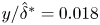 $y/\hat {\delta }^*=0.018$ and
  $\bar {w}/W_{\infty }=3.5\,\%$). The traversing system allows for shifting the imaging plane to different chord locations while maintaining the alignment and focus of the cameras and the laser. With this configuration, planes between 25 and 36 % of the chord are collected with an inter-spacing of 1 % of chord and a laser thickness of approximately 1 mm. Flow seeding is obtained by dispersing
  ${\simeq }0.5\ \mathrm {\mu }{\rm m}$ droplets of a water-glycol mixture in the wind tunnel through a SAFEX fog generator.
For each plane, 1000 image pairs are acquired at a frequency of 15 Hz and time interval of  $5\ \mathrm {\mu }{\rm s}$, corresponding to a free-stream particle displacement of almost 11 pixels. Each image pair is processed in LaVision Davis 10 through a multi pass cross-correlation with final interrogation window of
  $12\ {\rm px}\times 12\ {\rm px}$ and 50 % overlap, resulting in a final vector spacing of approximately
  $47\ \mathrm {\mu }{\rm m}$. The correlated velocity fields are then averaged and stitched through a Matlab routine delivering the time-averaged velocity components and identifying the wall location as the maximum light reflection region in the raw particle images.
With further processing of the velocity fields, the boundary layer mean velocity profiles ( $\bar {w}_z$) are obtained by averaging the
  $\bar {w}$ velocity signal along the z direction. The disturbance evolution profile in the wall-normal direction (
 $\langle \bar {w} \rangle _z$) is instead computed as the root mean square (r.m.s.) of the velocity signal along z at each fixed y-coordinate (e.g. Reibert et al. Reference Reibert, Saric, Carrillo and Chapman1996; Hunt & Saric Reference Hunt and Saric2011; Tempelmann et al. Reference Tempelmann, Schrader, Hanifi, Brandt and Henningson2012). Information on the dominant mode and its harmonics can be retrieved through a spatial Fourier analysis: at each y-coordinate the spanwise velocity signal is transformed in the spatial frequency domain (
 ${\rm FFT}_z(\bar {w})$), providing the spectra and the individual modes chordwise development. Moreover, the crossflow vortices amplitude can be estimated for each acquired plane by integrating the disturbance profiles along y up to the local
  $\delta _{99}$ (as suggested by Reibert et al. Reference Reibert, Saric, Carrillo and Chapman1996; Downs & White Reference Downs and White2013), providing an estimation of the modes’ chordwise growth and evolution (§ 3.3). The time-averaged displacement field uncertainty is estimated using the correlation statistics method (Wieneke Reference Wieneke2015), identifying an average uncertainty of
  $0.05\,\%W_{\infty }$ in the free stream and
  $0.10\,\%W_{\infty }$ in the BL region.
3. Steady perturbations characteristics
The following section is dedicated to the onset and evolution of crossflow disturbances as identified by IR and PIV measurements. An overview of the flow receptivity to the roughness arrays is reported, analysing the extracted transition fronts and the CFI growth.
3.1. Transition behaviour as a function of forcing amplitude and location
The IR visualization for the natural transition case (no DRE forcing) is reported in figure 3(a). The homogeneous temperature distribution suggests that the developing boundary layer is laminar throughout the imaged domain. Moreover, the characteristic light-dark streaks alternation typical of IR acquisition of CFI dominated BL (Dagenhart & Saric Reference Dagenhart and Saric1999) is largely absent in this visualization due to the weakness of the developing instabilities. A more deterministic flow scenario focused on a single monochromatic mode is obtained by applying a DRE array on the wing, as shown in the  $Re_k=24$ case reported in figure 3(b). The conditioned BL is characterized by a well-developed stationary CFI, visible as a streak alternation in the IR field, leading to the formation of the typical sawtooth transition front. Extending this analysis to the set of acquired IR images, the relative transition front location (
 $x_{{TR}}/c-x_{{DRE}}/c$) is estimated for all forced configurations considered, as reported in figure 4.

Figure 3. Infrared fields for (a) natural (i.e. no DRE) transition case; (b) forced transition case  $Re_k=24$. Flow comes from the left; the leading edge (blue line); DRE array location (yellow line); constant
  $X/c_X$ lines (-.).

Figure 4. Transition locations  $x_{{TR}}/c-x_{{DRE}}/c$ vs
  $Re_k$. Colourmap based on
  $x_{{DRE}}/c$, symbols based on element height. Cases with transition laying below the horizontal dashed line are super-critical (i.e. causing flow tripping).
The set of collected data identifies two main functional relations governing transition location, namely an increase (decrease) in element height and/or a decrease (increase) in streamwise location lead to an advancement (postponement) of laminar to turbulent transition. The employed metrics are not sufficient to deterministically predict the transition location. Nonetheless, despite the pronounced scatter observed in figure 4,  $Re_k$ qualitatively correlates to transition location. In particular, a critical behaviour is identified for forcing configurations with
  $Re_k\leqslant 190$, while arrays with higher
  $Re_k$ demonstrate a super-critical behaviour, causing transition shortly after the array location (
 $0\leqslant x_{{TR}}/c-x_{{DRE}}/c\leqslant 0.07$, Reibert et al. Reference Reibert, Saric, Carrillo and Chapman1996; Kurz & Kloker Reference Kurz and Kloker2016). These tripping configurations are neglected in the remainder of this work.
Considering these observations, it becomes evident that modifications of the crossflow-induced transition location due to DRE location and amplitude can not be simply approximated based on the local BL and geometrical scaling parameters of the roughness. Several factors can influence this behaviour, such as local pressure gradient, local boundary layer stability and near-DRE flow development. These effects can be responsible for modifying the effective initial perturbation amplitude introduced by the DRE and, thus, produce the observed spread in transition location. These amplitude modifications can then be associated to complex alterations of the flow and of the instabilities development induced by the specific forcing configuration applied, as can be further assessed considering the collected PIV data and performed stability analysis.
3.2. Mean flow development
Prior to the description of steady perturbations, the development of the time- and spanwise-averaged velocity fields within the PIV measurement domain is outlined. In particular, the present study investigates a wide range of chord locations for the DRE arrays application, namely from  $x/c=0.02$ to 0.35 for which a LPSE solution accounting for the local pressure gradient is computed (figure 1). To confirm that comparable stability conditions pertain the experimental boundary layer, the naturally growing BL (i.e. no forcing applied) measured through PIV is compared with the numerical solution on which stability is solved. Figure 5(b) collects the numerical and experimental BL velocity profiles estimated at
  $x/c=0.35$, ensuring a good match is achieved as further shown by the chordwise evolution of the BL geometrical parameters (figure 5c). Finally, to assess that the natural BL features are repeatable throughout the different forcing cases considered, the
  $\overline {w}_z$ velocity profiles for the natural transition case and for the forcing case featuring arrays placed at
  $x_{{DRE}}/c=0.30$ (
 $Re_k=64$) are compared (figure 5a). The reported
  $\bar {w}_z$ profiles for this downstream forcing (for which no DRE is applied at the leading edge) develop as the natural one upstream of the array location. Hence, the base flow repeatability allows for a systematic comparison of the flow modifications introduced by the different forcing configurations.

Figure 5. (a) Plot of  $\bar {w}_z$ from numerical solution (solid line), PIV for natural transition (-
 $\circ$) and PIV for
  $Re_k=64$ (with
  $x_{DRE}/c=0.3$,
  $\diamond$). (b) Plot of
  $\bar {w}_z$ from numerical solution (solid line), from PIV for natural transition (
 $\square$) and PIV for
  $Re_k=24$ (
 $\times$). Only 1 in 3 marks are shown in the y direction. (c) Boundary layer integral parameters from numerical
  $\bar {w}$ (full lines) and from PIV (symbols).
The  $\bar {w}$ velocity contours acquired at
  $x/c =0.25$, 0.30 and 0.35 for three representative forcing cases with
  $Re_k$ in the critical range are reported in figure 6. The mean boundary layer velocity distribution
  $\bar {w}_z$ for the
  $Re_k=24$ case is also reported in figure 5(b). In contrast to the clean case, the forced BL velocity profiles feature an inflection point (already present at
  $x/c=0.25$) and undergo further distortion moving downstream, indicating nonlinearities are strongly affecting the forced scenario. This poses a limit for linear approaches to stability theory, warranting nonlinear extensions computed through NPSE solutions, as further discussed in § 3.3. Moreover, the forced boundary layer is thicker than the corresponding clean case and achieves a higher slope close to the wall, corresponding to an increased local skin friction coefficient. These modifications can be related to the onset of turbulent motions introduced by the strong instabilities and nonlinearities characterizing the flow. These features also reflect in the development of the PIV disturbance profiles, as supported by the modes’ growth and evolution analysed in the next section.

Figure 6. Contours of  $\bar {w}$ velocity fields acquired for (a–c)
  $Re_k=18$; (d–f)
  $Re_k=24$; (g–i)
  $Re_k=155$. Particle image velocimetry plane location: (a,d,g)
  $x/c=0.25$; (b,e,h)
  $x/c=0.30$; (c, f,i)
  $x/c=0.35$.
3.3. Stationary crossflow instabilities growth
As described in § 2.4.2, a Fourier spatial decomposition procedure is applied to all collected PIV planes, characterizing the modes’ evolution along the chord for each forcing case. The resulting spatial spectra is reported in figure 7(a) for the representative forcing configuration  $Re_k=24$. As expected, the dominant peaks correspond to mode
  $\lambda _1$ and its harmonics (
 $\lambda _2$ and
  $\lambda _3$), all growing along the wing chord.

Figure 7. (a) Fourier spectra in the spanwise wavelength domain and experimental disturbance profiles at (b)  $x/c=0.25$; (c)
  $x/c=0.35$ for
  $Re_k=24$. Plot of
  $\langle \bar {w} \rangle _z$ from PIV (–), from two Fourier reconstructed profiles
  $\langle \bar {w}_{R_{1}} \rangle _z$ (
 $\square$) and
  $\langle \bar {w}_{R_{1,2,3}} \rangle _z$ (
 $\ast$) and NPSE result (-.). Only 1 in 3 marks are shown along y. Experimental
  $\delta _{99}$ (- -).
Within the spatial Fourier domain each mode can be independently extracted and analysed. Hence, through an inverse Fourier transform the time-averaged velocity fields  $\bar {w}_{R_{i}}$ can be reconstructed as only composed by a chosen truncated ensemble of modes of interest i. Figure 7(b–c) shows the r.m.s. disturbance profiles
  $\langle \bar {w} \rangle _z$ computed for the reference forcing case from the
  $\bar {w}$ PIV fields. This is compared with the disturbance profiles extracted from two fast Fourier transform (FFT) reconstructed fields:
  $\bar {w}_{R_{1}}$ including only the
  $\lambda _1$ mode and
  $\bar {w}_{R_{1,2,3}}$ additionally accounting for
  $\lambda _2$ and
  $\lambda _3$ harmonics. Despite small discrepancies in their maximum amplitude, the three disturbance profiles have similar shape, growing along the chord and featuring a secondary local maximum related to nonlinear interactions. The mild amplitude differences reduce as more modes are included in the FFT flow reconstruction, even if the
  $\lambda _1$ mode is already capturing all of the main flow features. The
  $\lambda _1$ mode shape function extracted from the NPSE solution at the corresponding chord locations shows a satisfactory matching behaviour, despite mild over-prediction of mode growth by the numerical solution. Similar discrepancies are also observed by Haynes & Reed (Reference Haynes and Reed2000), and can be attributed to the small differences between the experimental and numerical base flow and to the actual wing curvature.
For a more quantitative analysis, the instability amplitude and growth are estimated following the integral amplitude approach proposed by Downs & White (Reference Downs and White2013). Having confirmed the  $\lambda _1$ mode gives the main contribution to the disturbance amplitude and its development, for the remainder of this work, the amplitudes estimations presented are extracted from the
  $\bar {w}_{R_{1}}$ and
  $\bar {w}_{R_{2}}$ reconstructed flow fields unless otherwise specified. This procedure is akin to the amplitude estimation from the computed NPSE solutions, allowing for a direct comparison of the numerical and experimental results. Moreover, propagating the PIV uncertainty error in the amplitude calculation, the error range pertaining the extracted amplitude values can be estimated, reaching a mean value of
  $\pm$1 %. Repeating the amplitude estimation procedure for the acquired cases the
  $A_{int}$ curves reported in figure 8 are obtained, showing the effect of different forcing configurations on the generated disturbances evolution.

Figure 8. Integral perturbation amplitude along x from (a–c)  $\bar {w}_{R_1}$ fields and (d–f)
  $\bar {w}_{R_2}$ fields. Columns refer to a fixed
  $k$, matching NPSE solution (- - lines), NPSE solution sensitivity (shaded regions), NPSE initial amplitude estimations (full markers). Data relative to
  $x/c$ locations downstream of the transition point are excluded from the plot.
In the most upstream forcing configurations, the instabilities grow throughout the domain up to a saturation amplitude level. In agreement with previous studies (Reibert et al. Reference Reibert, Saric, Carrillo and Chapman1996; Haynes & Reed Reference Haynes and Reed2000; White et al. Reference White, Saric, Gladden and Gabet2001) for this subset of cases the forced primary structures reach saturation at comparable amplitude values ( $A_{int, saturation} \simeq 0.06W_{\infty }$), independent of the forcing amplitude and location. These cases are accompanied by the growth of the
  $\lambda _2$ mode, which also saturates for the more upstream configurations. However, forcing at more downstream chord locations as well as with higher DRE arrays, leads to lower saturation amplitudes. This different behaviour can be attributed to several reasons, among which the breadth of the parameter range involved which may lead to variations in the receptivity process. Moreover, cases with
  $Re_k \geqslant 24$, 90, 160 respectively for the three different heights considered, are as well affected by the early amplitude saturation and subsequent decay. Such behaviour is indicative of the later stages of transition and onset of turbulence, which essentially breaks the spanwise coherence of the structures. Instead, with a further downstream shift (i.e.
  $Re_k \leqslant 18$, 70, 150) arrays of all considered heights induce instabilities that grow along the whole PIV domain without reaching saturation, accompanied by a negligible or absent development of the
  $\lambda _2$ mode.
Most of the measured upstream forcing configurations are characterized by well-developed  $\lambda _2$ modes, indicating the boundary layer flow is affected by nonlinearities. Therefore, for each of these cases, an NPSE stability solution is computed (§ 2.2). The numerical amplitudes computed from NPSE solutions are reported for all the tested cases in figure 8. Figure 9 instead, shows the specific comparison between NPSE, LPSE and PIV computed amplitudes,
  $N$-factor and shape functions evolution for an upstream (
 $Re_k=24$) and a downstream (
 $Re_k=18$) forcing configuration. Overall, mild amplitude differences are observed in figures 8 and 9, mostly attributed to mild base flow discrepancies, possibly enhanced downstream of the roughness element due to the complex physics of the near-DRE flow region (as discussed in § 4). Additionally, the actual wing curvature as well as the experimental uncertainty on the roughness height and exact chord location can also contribute to the observed differences. More significant discrepancies characterise the
  $Re_k\geqslant 160$ cases. The pronounced discrepancies between experimental and numerical results at higher
  $Re_k$ reveal possible effects near the DRE which are not modelled by the NPSE approach. Among others these can include unsteadiness in the wake (e.g. vortex shedding) and non-modal effects in the stationary vortex system, as further discussed in § 4.

Figure 9. Particle image velocimetry and NPSE  $\lambda _1$ mode (a)
  $N$-factor and (d) amplitude curves for
  $Re_k=24$ (
 $\circ$) and
  $Re_k=18$ (
 $\ast$) with
  $x_{{DRE}}/c$ (-.-),
  $A_0$ (
 $\times$). (b–e) Shape functions of the
  $\lambda _1$ and (c–f)
  $\lambda _2$ mode at
  $x/c=0.30$ for the NPSE (full line), LPSE (- -) and Fourier shape functions from experimental data (symbols). Experimental
  $\delta _{99}$ (horizontal - -), NPSE matching sensitivity (shadowed areas).
Notwithstanding mild topological differences, the NPSE correctly predicts the instability saturation amplitude ( $A_{int, saturation} \simeq 0.057W_{\infty }$,
 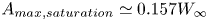 $A_{max, saturation} \simeq 0.157W_{\infty }$ in agreement with Reibert et al. Reference Reibert, Saric, Carrillo and Chapman1996). The
  $\lambda _2$ harmonic and its evolution are also properly described, despite enhanced amplitude differences for the more upstream configurations considered, related to the primary amplitude discrepancies. To verify the sensitivity of the NPSE matching to the initial amplitude estimate, the area between the matching NPSE solution and two equivalent solutions initiated with
  $A_0 \times \ (1 \pm 0.1)$ is shown as a shaded region in figure 8. In addition, the experimental amplitude uncertainties given by the PIV correlation have been found to be smaller, thus contained also in the shaded region.
The overall instability behaviour is well modelled by the NPSE (as already shown by Haynes & Reed Reference Haynes and Reed2000). Therefore, the upstream portion of the numerical solution can be exploited to extract an estimation of the perturbation initial amplitude  $A_0$. This is computed as the equivalent amplitude a modal CFI should posses at the
  $x_{DRE}/c$ location in order to give a downstream development of the flow field comparable to the experimental measurement. This is particularly instructive given the inability of experimental measurement techniques to resolve such mild effects. It must be noted that all NPSE simulations are initiated only with the
  $\lambda _1$ mode and as such
  $A_0$ refers to the latter. The
  $A_0$ extracted for the two cases of figure 9(d) are represented by the red
  $\times$ markers, while the ensemble estimates for the various tested heights and chord locations are reported in figure 10.

Figure 10. Initial instability amplitude ( $A_0$) from NPSE against
  $Re_k$. Dashed line is a linear fit of the
  $A_0$ data (
 $A_{0,{fit}}$). Colourmap based on
  $x_{{DRE}}/c$, symbols based on element height.
The observed  $A_0$ curves immediately confirm that the receptivity process is not linearly dependent on the considered parameters. Nonetheless,
  $Re_k$ appears to correlate surprisingly well to the estimated initial amplitude, possibly due to the inherent information used by this metric which includes the local velocity or momentum of the incoming flow. Despite not giving a complete description of the single forcing cases behaviour, the simple least-squares linear data fit (
 $A_{0,{fit}}=6.2\times 10^{-5}Re_k$) reported in figure 10 appears to capture the main
  $A_0$ differences given by modifications of the DRE amplitude. A global estimation of the fit accuracy is described by the coefficient of determination (
 $R^2=0.97$), indicating the fit is capturing up to 97 % of the data variance. More detailed considerations can be carried out considering the
  $A_0$-linear fit local residuals (
 $\Delta A_0=A_0-A_{0,{fit}}$), which appear to be relatively higher for the smaller elements. In particular, for
  $k_1$, the residuals estimation reaches a maximum of
  $\Delta A_0\simeq 0.5A_0$ in contrast to the
  $\Delta A_0\leqslant 0.25A_0$ for
  $Re_k>70$. Additionally, for each of the three considered element amplitudes, higher deviations from the linear fit pertain to the more upstream configurations reported, which experience stronger local pressure gradient variations and possible local effects not properly modelled by the NPSE approach. This behaviour is in agreement with previous investigations stating that in the vicinity of the dominant mode neutral point, linear receptivity is only expected for DRE amplitudes much smaller than those of the present study (Schrader et al. Reference Schrader, Brandt and Henningson2009; Kurian et al. Reference Kurian, Fransson and Alfredsson2011; Tempelmann et al. Reference Tempelmann, Schrader, Hanifi, Brandt and Henningson2012). The more downstream cases, however, are less affected by the local flow field characteristics (i.e. pressure gradient and local effects), falling closer to the linear fit approximation for the
  $Re_k-A_0$ relation. This behaviour validates the possibility of up-scaling the upstream configurations to further investigate the near-DRE flow phenomena, and reflects the monotonic behaviour of transition location with
  $Re_k$ observed from the IR measurements (figure 4).
Notwithstanding geometrical parameters, the direct solution of nonlinear stability theory appears to capture best the overall increase of initial amplitude corresponding to the three considered heights simply based on downstream measurements. Yet, the initial amplitude values are not linearly dependent on k, as the relative increase between estimated amplitudes is not representative of the proportional increase in DRE height (Tempelmann et al. Reference Tempelmann, Schrader, Hanifi, Brandt and Henningson2012, table 2). In addition, the DRE location also appears to affect the initial amplitude estimation, showing an initial increase in  $A_0$ followed by a slow decrease as more downstream application locations are considered. However, DREs of higher amplitude placed at identical
  $x_{DRE}/c$ (thus, identical pressure gradient) lead to stronger differences between the NPSE and experimental amplitudes evolution (figure 8). The observed trends significantly differ from the results obtained by Tempelmann et al. (Reference Tempelmann, Schrader, Hanifi, Brandt and Henningson2012) for smaller roughness heights (i.e.
  $\leqslant$10 % of the local
  $\delta ^*$) that led to a linear receptivity process. This different correlation between
  $A_0$ and the elements’ location further suggests that the DRE amplitude is the dominant parameter for the receptivity of the cases considered in this work. Multiple error sources can be affecting the
  $A_0$ behaviour, including measurement uncertainties and modelling errors in the NPSE approach which, for example, does not account for the effect of the local pressure gradient on the near flow dynamics and consequently on
  $A_0$. In fact, a good match between numerical and experimental amplitude is obtained to 1 % of chord downstream of the array location, as shown by the full marks of figure 8. However, by comparing the amplitude values closer to the element (i.e. 0.3 % downstream of the element, figure 13) differences between the experimental and the NPSE values can be observed, confirming modal stability theory does not accurately model the instability growth immediately aft of the roughness array. These observations further justify the identified
  $A_0$ behaviour, stressing the importance of the near-DRE flow dynamics for the onset and later evolution of stationary CFI.
In conclusion, the investigation of the stationary disturbances led to the description of the downstream development of the primary mode and its harmonics. Moreover, complementing NPSE simulations allows for the estimation of the initial instability amplitude represented by  $A_0$. As expected, the reported values show a strong dependency of the instability onset on the forcing amplitude being, however, only mildly affected by the forcing location. Yet, the defined geometrical parameters are not capable of completely describing the underlying receptivity relations. This can be traced back to the flow field dynamics in the immediate vicinity of the DRE, which can be affected by the local pressure gradient and potentially include non-modal and transient growth features similar to what was identified in 2-D flows by White, Rice & Ergin (Reference White, Rice and Ergin2005) and Reshotko (Reference Reshotko2001). The
  $A_0$ estimation directly from NPSE appears to support this hypothesis, therefore, a further step towards the analysis of the relation between the DRE element and the initial instability amplitude can be guided by the near-DRE flow investigation reported in § 4.
4. Near-DRE flow development
Of the results reported so far, only the  $A_0$ estimation brings interesting insights on the initial phases of receptivity. However, despite observing a dependency on the forcing amplitude and location, the
  $A_0$ modifications appear to be mostly affected by the near-element flow dynamics, characterized by flow phenomena that can hardly be parametrized. Nonetheless, to better understand the initial receptivity phases, the last part of this work is dedicated to a more in-depth investigation of the flow evolution in the roughness elements vicinity. For arrays applied between
  $x/c=0.25\text {--}0.30$, additional PIV planes are collected with a step
  $\simeq$0.16 % chord starting 0.3 % downstream of the DRE location to avoid light reflections.
The time-averaged spanwise  $\bar {w}$ velocity contours for forcing at
  $Re_k=145$ (
 $x_{DRE}/c=0.25, k_3$) are reported in figure 11 along with the corresponding perturbation fields (estimated as
  $\bar {w}(z,y)-\bar {w}_z(y)$). This forcing case is chosen as the representative configuration throughout this section as it features the larger element considered (i.e.
  $k_3$), thus, the developing flow features are most observable and less subject to noise issues. The average velocity fields reveal a boundary layer almost unaffected by CFI, in fact no flow modulation is yet present in the base flow. However, a momentum deficit region is developing directly in the wake of the element surrounded by higher speed flow possibly due to a momentum redistribution effect induced by the roughness element itself (Kurz & Kloker Reference Kurz and Kloker2016). Already visible in the plane closest to the DRE (at
  $x/c=0.253$) this low-speed hump forms immediately downstream each of the elements present in the PIV domain and rapidly decays between
  $x/c=0.253\text {--}0.26$. Downstream (
 $x/c=0.27$) the disturbance field evolves into a weak but uniform high-speed low-speed region alternation typical of stationary CFI (e.g. Bippes Reference Bippes1999). The topology of the flow modulation is very similar to corresponding cases of weak upstream forcing such as
  $Re_k=18$ shown in figure 6. These observations reconcile well with the DNS results by Kurz & Kloker (Reference Kurz and Kloker2016). More specifically, they identified two pairs of horseshoe vortices developing around the roughness elements: an outer pair propagating from the element sides, most likely due to the element-induced spanwise shear, and an inner pair originating aft of the element due to wall-normal ejection of flow. In a 3-D boundary layer for both pairs, only the leg co-rotating with the BL crossflow is sustained and develops along the chord, while the counter-rotating legs are suppressed shortly after the elements location. The emergence of these vortices drives a momentum redistribution process which results in the formation of a low-speed hump in the wake of the elements due to low-momentum flow upwelling. Despite the different flow features characterizing a 2-D or 3-D boundary layer, Kurz & Kloker (Reference Kurz and Kloker2016) observed that the near-DRE flow characteristics are comparable for the two cases. In fact, flow features and evolution comparable to what is observed in the present work, are reported in the work by Ergin & White (Reference Ergin and White2006), an experimental investigation on the flow past a roughness element in a 2-D boundary layer.

Figure 11. (a–c) Time-averaged spanwise  $\bar {w}$ velocity contours and (d–f) perturbation velocity fields (
 $\bar {w} - \bar {w}_z$) acquired for
  $Re_k=145$ in the array vicinity. Superimposed contours of
  $\bar {w}$ (full lines, 5 levels from 0 to 1). Dashed rectangle represents the roughness shape and location.
A spanwise Fourier decomposition is applied to these near-DRE fields and the corresponding spectra are reported in figure 12 for case  $Re_k=145$. Differently from the upstream forcing case (figure 7a), the spectra of the present case identify a high energy spectral content involving the dominant mode
  $\lambda _1$ and numerous harmonics. This is mainly attributed to the highly concentrated region of velocity deficit in the wake of the elements, which are otherwise located in an undisturbed spanwise invariant flow. In terms of spatial spectra, the DRE wake essentially acts as a pseudo-pulse, effectively containing all spatial frequencies. The diameter of the DRE (
 $\simeq$1.7 mm) is nevertheless finite and only four times less than the elements inter-spacing. As such, the spectral energy is not equally distributed and decays with higher harmonics. For the results presented in figure 12, more than 35 % of the spectral energy is contained in the first five harmonics. However, it must be noted that the identified spectral components do not necessarily correspond to natural modal instabilities in the flow, rather they can be seen as modal representations of the near-DRE wake in Fourier space. As such, the perturbation amplitude computed following the integral approach includes all the complex flow features corresponding to the near-DRE flow development. Integral amplitudes extracted from the
  $\bar {w}$ velocity fields and from the
  $\bar {w}_{R_1}$ field are reported in figure 13.

Figure 12. (a) Fourier spectra in the spanwise wavelength domain and (b) spectra amplitudes in the x– $\lambda _z$ plane for
  $Re_k=145$.

Figure 13. Integral amplitude along x in the array vicinity from (a)  $\bar {w}$, (b)
  $\bar {w}_{R_1}$. Integral amplitudes from the NPSE solution at
  $x/c=0.253$ (full markers).
The amplitude development extracted from the time-averaged PIV fields displays a very mild total disturbance growth followed by a significant decay associated to the velocity deficit evolution, and a subsequent growth due to the flow modulation development, figure 13(a). As also confirmed by the reported spectra, the downstream flow modulation is dominated by the  $\lambda _1$ mode and despite overall smaller amplitudes it reflects the crossflow characteristics and growth process previously discussed for cases of more upstream located arrays (figure 6). Interestingly, the amplitude curves of the presented cases are characterized by comparable trends and amplitudes in the element vicinity. The change of height or chord locations of these arrays leave the initial decay and subsequent growth almost unaltered, suggesting that the near-DRE flow region is mostly influenced by the flow blockage caused by the element itself rather than the overall flow stability. Unfortunately, the current set-up does not permit to directly compute experimental instability amplitudes for arrays located in regions affected by stronger variation of the pressure gradient as these are located closer to the leading edge, where the boundary layer is extremely thin. However, the observed near-DRE flow similarity is in agreement with the results of the numerical computations conducted by Kurz & Kloker (Reference Kurz and Kloker2014) on a more upstream forcing configuration, and sets an important starting point for the scalability of the examined configurations.
The similarity among forcing cases is additionally evident on the amplitude curves extracted from the  $\bar {w}_{R_1}$ fields (figure 13b). It must be emphasised that the identified Fourier modes do not necessarily represent the naturally developing wake instabilities. Nonetheless, they provide a valid modal description of the wake flow field which delivers interesting insights in the relative flow dynamics. In particular, for the three presented configurations, the
  $\lambda _1$ mode shows a continuous decay from the DRE location to 1 % of chord downstream, indicating that the initial amplitude growth observed in figure 13(a) may be linked to the behaviour of higher harmonics. To further address this consideration, hereafter we present a more detailed analysis of the individual Fourier modes’ behaviour for case
  $Re_k=145$. Figure 14 includes the estimation of the total perturbation integral amplitude
  $A_{int}(\bar {w})$, as well as the integral amplitude of the first six harmonics of the dominant mode
  $\lambda _1$ extracted from the Fourier spectra. Additionally,
  $A_{int}(\bar {w}_{R_{1-6}})$ is the integral amplitude computed from a truncated Fourier reconstructed flow field including only the six reported modes. Despite the mild amplitude differences between
  $A_{int}(\bar {w})$ and
  $A_{int}(\bar {w}_{R_{1-6}})$, both amplitude trends show a mild growth followed by rapid decay in the element vicinity. However, both the
  $\lambda _1$ and
  $\lambda _2$ modes are decaying aft of the roughness element, and only start to grow downstream of
  $x/c=0.26$, where the NPSE-experimental amplitude match indicates that the instability growth is following an exponential trend. On the other hand, in the element vicinity (i.e.
  $x/c<0.26$) Fourier modes
  $\lambda _3$,
  $\lambda _4$,
  $\lambda _5$ and
  $\lambda _6$ all show mild growth followed by rapid decay. These flow features match well with the results presented by White et al. (Reference White, Rice and Ergin2005), who identified non-modal mechanisms and, in particular, transient growth as a fundamental feature of the near-DRE wake development for a non-swept flow. The individual modes behaviour described in figure 14 as well as the observed mild
  $A_{int}(\bar {w})$ growth, appear to reflect the characteristics of a transient growth process (e.g. Landahl Reference Landahl1980; Schmid & Henningson Reference Schmid and Henningson2001) possibly driven by the behaviour of individual Fourier components comparable to those identified by White et al. (Reference White, Rice and Ergin2005).

Figure 14. Integral amplitude along x in the array vicinity for forcing case  $k_3$,
  $Re_k=145$ from
  $\bar {w}$,
  $\bar {w}_{R_1}$,
  $\bar {w}_{R_2}$,
  $\bar {w}_{R_3}$,
  $\bar {w}_{R_4}$,
  $\bar {w}_{R_5}$,
  $\bar {w}_{R_6}$ flow fields and from the Fourier reconstructed flow field
  $\bar {w}_{R_{1-6}}$. Amplitude of matching NPSE solution (-.). The y-axis is plotted with a logarithmic scale to ease visualization.
Previous works by Corbett & Bottaro (Reference Corbett and Bottaro2001) and Breuer & Kuraishi (Reference Breuer and Kuraishi1994) show that flow fields developing aft of a cylindrical element can produce a transient growth mechanism that can lead to rapid initial growth of crossflow instabilities, enhancing their downstream development which then follows an exponential growth process. This transient growth process is typically governing the linear superposition of non-orthogonal modes (e.g. Corbett & Bottaro Reference Corbett and Bottaro2001; Levin & Henningson Reference Levin and Henningson2003; Lucas Reference Lucas2014), thus, it would relate the amplitude growth observed in the element wake to the presence of non-modal flow interactions. More specifically, the vectorial sum of individually decaying non-orthogonal solutions to the stability problem can lead to transient growth. However, these eigensolutions appear at the same spanwise wavelength and frequency. As such, the decoupling of modal (i.e. exponential) and non-modal (i.e. algebraic) growth effects is not possible by means of a Fourier decomposition. Non-modal interactions are not accounted for in the NPSE solver, however, together with the local pressure gradient they could significantly affect the near-DRE wake development, further justifying the  $A_0$ behaviour observed in figure 10. Additionally, the initial boost in amplitude of higher harmonics of the primary stationary mode given by a transient growth mechanism can lead to the formation of strong shear layers in the DRE wake. These can in turn induce unsteady wake instabilities (such as vortex shedding or shear layer instabilities of sinuous or varicose nature) that can affect the CFI initial amplitude, growth rate and transition location (Breuer & Kuraishi Reference Breuer and Kuraishi1994; Lucas Reference Lucas2014; Loiseau et al. Reference Loiseau, Robinet, Cherubini and Leriche2014). In particular, in the
  $Re_k=145$ forcing case presented in figure 14 the effect of the transient mechanism on the primary wavelength (i.e.
  $\lambda _1$) is visible in the initial decay. The latter cannot be modelled by NPSE, as is evident from the different evolution of
  $A_{int}(\bar {w}_{R_{1}})$ and the integral amplitude computed from the NPSE solution, i.e.
  $A_{NPSE}(\bar {w}_{R_{1}})$. The NPSE amplitude evolution is in fact purely exponential, thus resulting in an underestimation of the
  $\lambda _1$ mode
  $A_0$. This consideration explains the observed numerical and experimental amplitude differences registered in figure 13(b), where the NPSE initial amplitude is underestimated for all the reported cases if compared with the experimental values. The result in figure 14 is possibly the first experimental observation of transient growth in a swept wing boundary layer. Nevertheless, the region in which the perturbation amplitude initially grows while individual modes are decaying is extremely short (less than 1 % chord). This spans merely three PIV measurement planes rendering the spatial resolution insufficient to identify one of the signature features of transient growth which is algebraic amplitude evolution. The elucidation of such mechanisms is currently the subject of dedicated ongoing investigations by the authors.
In conclusion, for the limited number of cases investigated in this study, the application of DRE in a region affected by linearly developing natural crossflow is still successfully conditioning the downstream CFI development. Moreover, the pre-existing CFI modulation appears to have negligible effects on the near-DRE flow features which present comparable amplitude and behaviour independently of the forcing chord location, as also observed by Kurz & Kloker (Reference Kurz and Kloker2014). Therefore, the withstanding relation between roughness elements and crossflow onset may be more complex than a simple two elements interaction, involving a chain of effects moving from the elements to the near-DRE flow and consequently to the onset of the CFI. The identified near-DRE behaviour can potentially be linked to a transient growth process which affects the BL flow providing the proper initial conditions to the modal crossflow instabilities development (e.g. Corbett & Bottaro Reference Corbett and Bottaro2001). Considering the narrow parameter range examined and the insufficient spatial resolution for the current work this remains a hypothesis. However, its potentially pertinent role in the complete definition of the receptivity process justifies further detailed investigations dedicated to the near-DRE flow field. These investigations can be simplified by the observed repeatability of the near-DRE wake characteristics demonstrated in this work, allowing for this type of measurement at more downstream and experimentally more accessible chord locations.
5. Conclusions
The presented experimental investigations explore the overall effect of DRE amplitude and chord location on the development and breakdown of stationary CFI. Roughness arrays are manufactured with a fixed element inter-spacing corresponding to the wavelength of the dominant crossflow mode ( $\lambda _1$ according to LPSE), in order to force a deterministic flow scenario focused on a single monochromatic mode. The forcing arrays are applied on the wing surface at various chord locations, while four different element heights are considered spanning a broad range of
  $k/\delta ^* \simeq 0.15\text {--}2.4$ and
  $Re_k \simeq 15\text {--}280$.
The global inspection of transition performed through IR thermography relates the forcing configuration to the observed transition modifications. An increase (decrease) in element height and/or a decrease (increase) in DRE streamwise location lead to an advancement (postponement) of laminar to turbulent transition. Reflecting the transition front modifications, configurations characterized by higher  $Re_k$ introduce instabilities with higher amplitudes which rapidly grow along the chord up to saturation and turbulence onset.
Nonlinear development of primary instabilities is numerically modelled by solving NPSE through an in-house developed solver. A good match is found between the experimental and numerical development of the instabilities as they progress in the boundary layer, including the extracted instabilities amplitude and saturation amplitudes. As such, the upstream initialisation of the numerical solution provides an estimation of the equivalent instability initial amplitude ( $A_0$) at the DRE array location leading to comparable downstream development of CFI. The collected
  $A_0$ values indicate the forcing amplitude is the main parameter influencing the initial instability amplitudes. The direct estimation of
  $A_0$ using NPSE appears to capture the overall influence of the forcing elements sufficiently well, while still revealing pertinent differences from a universal scaling law. In particular, the inherent relations between forcing configuration and the initial instability amplitudes as well as the transition locations are not following a simply linear trend. Nonetheless,
  $Re_k$ performs relatively well in capturing both transition modifications and estimation of the initial perturbation amplitude stemming from a given DRE configuration. However, the residual data scatter suggests more complex and possibly non-modal mechanisms, likely influenced by the local pressure gradient and not captured by the NPSE, are active in the element vicinity.
The final part of this work presents an investigation of the near-DRE flow development for a limited set of cases. In the velocity fields a momentum deficit region is identified behind the element and is observed to decay further downstream, where a boundary layer modulation corresponding to a stationary crossflow mode (with  $\lambda _1$ wavelength) emerges (Kurz & Kloker Reference Kurz and Kloker2016). These flow features are reflected by the reported amplitude estimations. Additionally, DRE arrays are applied in a region affected by the development of weak (i.e. still linear) natural crossflow disturbances, conditioning the CFI evolution also in this configuration. This confirms the near-DRE flow is mostly influenced by the blockage effect of the element rather than the local flow stability, further reconciling the inability of NPSE back projections in fully capturing the initial amplitude (
 $A_0$). Furthermore, this observation opens new possibilities for up-scaling of the considered forcing configurations, which would simplify the experimental investigation of the near-DRE flow features. Moreover, preliminary evidence of transient growth behaviour can be identified in the DRE wake, based on spanwise spectral analysis. However, the few cases considered and the low spatial resolution achieved require further dedicated investigations to confirm this hypothesis.
From the reported results it appears that the inherent relation between roughness elements and CFI onset is more complex than a simple two elements interaction. A chain of effects relating the physical elements to their near-DRE flow features and consequently to the onset of the CFI is revealed, effectively making the near-DRE flow development an intermediate and important receptivity step. This step is eventually responsible in setting the initial conditions for the modal CFI development. Considering their pertinent role in the complete definition of the receptivity process, near-DRE dynamics will be the subject of future investigations. These investigations can be simplified by the revealed repeatability of the flow characteristics, enabling such measurements at more downstream and experimentally more accessible chord locations.
Acknowledgements
A dedicated acknowledgement goes to S. Bernardy and E. Langedijk for sharing their technical knowledge during the experimental preparation and to the colleagues for their contribution and support.
Funding
The authors are grateful to the European Research Council for financially supporting this research through the GloWing Starting Grant (grant no. 803082).
Declaration of interests
The authors report no conflict of interest.


 Open access