


Introduction
Calving is an important mechanism of mass loss for marine-terminating Arctic glaciers, including those of the Russian Arctic (Moholdt and others, Reference Moholdt, Heid, Benham and Dowdeswell2012a; Melkonian and others, Reference Melkonian, Willis, Pritchard and Stewart2016). The Russian Arctic, which comprises the archipelagos of Novaya Zemlya, Severnaya Zemlya and Franz Josef Land (Fig. 1a), had a total glacierized area of 51 592 km2 during the period 2000–2010 with tidewater glaciers accounting for 65% of this area (Pfeffer and others, Reference Pfeffer2014). The estimated total ice volume in the Russian High Arctic is 16 839 ± 2205 km3 (Huss and Farinotti, Reference Huss and Farinotti2012). In spite of recent climate warming over the Arctic region (Hartmann and others, Reference Hartmann2013), the recent ice-mass losses from the Russian Arctic were moderate, totalling ~ 11 ± 4 Gt a−1 over 2003–2009 (Moholdt and others, Reference Moholdt, Wouters and Gardner2012b; Matsuo and Heki, Reference Matsuo and Heki2013; Gardner and others, Reference Gardner2013). This is far less than other Arctic regions such as the Canadian Arctic, Greenland peripheral glaciers and glaciers of Alaska, even if considered per unit area (Gardner and others, Reference Gardner2013). However, the mass losses from the Russian Arctic by the end of the 21st century have been projected to increase substantially (Radić and others, Reference Radić2013), with an expected contribution to sea-level rise of between 9.5 ± 4.6 and 18.1 ± 5.5 mm in sea-level equivalent over 2010–2100, depending on emission-pathway scenarios (Huss and Hock, Reference Huss and Hock2015).
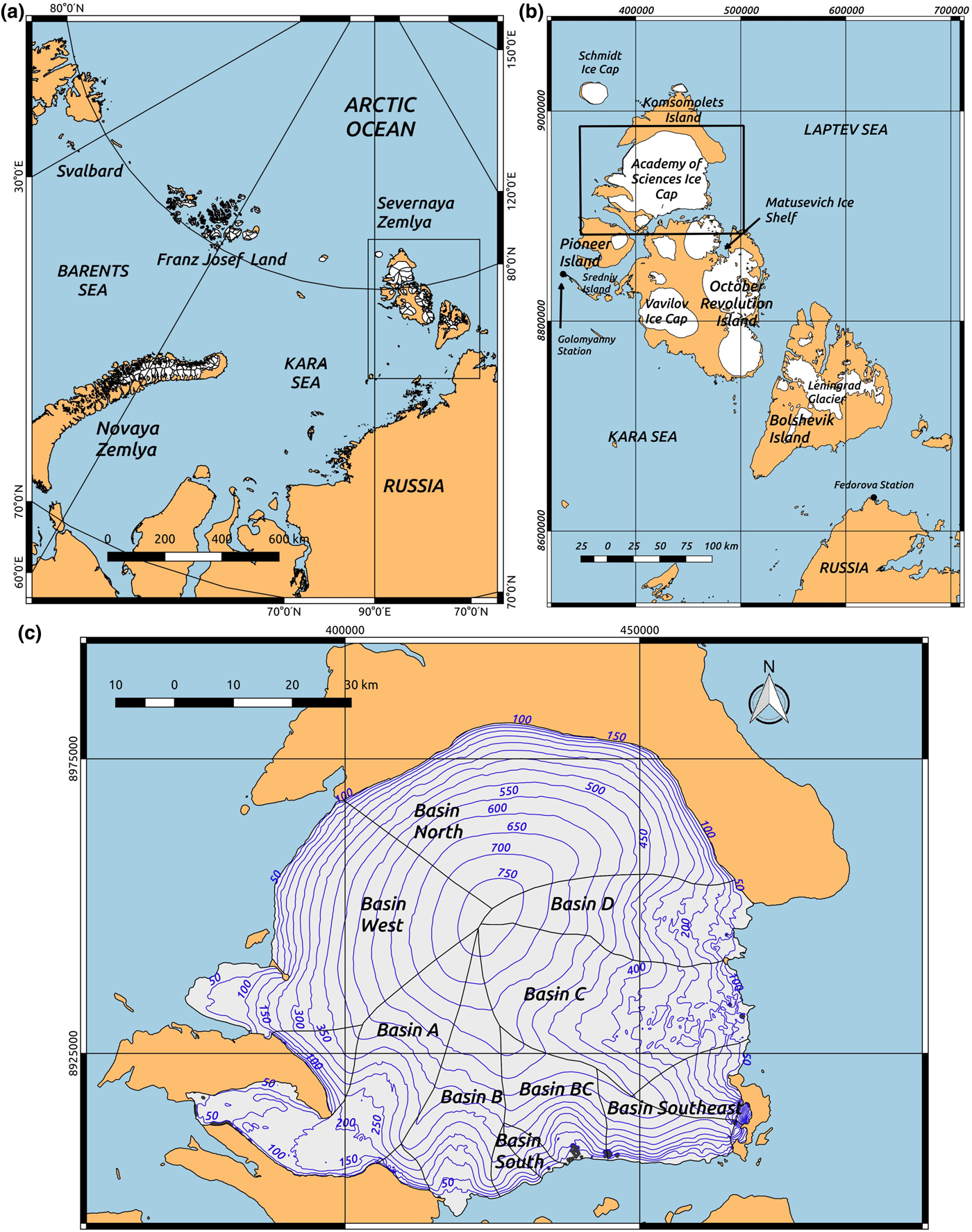
Fig. 1. (a) Location of Severnaya Zemlya in the Russian Arctic. (b) Major ice masses on Severnaya Zemlya (Wessel and Smith, Reference Wessel and Smith1996). Glacier outlines are from the Randolph Glacier Inventory (RGI) version 5.0 (Pfeffer and others, Reference Pfeffer2014). (c) Surface topography of the Academy of Sciences Ice Cap in Severnaya Zemlya from ArcticDEM mosaic product (Noh and others, Reference Noh, Howat, Porter, Willis and Morin2016). Outlines defining the various drainage basins of the ice cap are from the RGI. Basins A, B, C and D are named following Dowdeswell and others (Reference Dowdeswell2002) and Moholdt and others (Reference Moholdt, Heid, Benham and Dowdeswell2012a). The basin between Basins B and C is referred to here as Basin BC and new names Basin West, Basin South and Basin Southeast are introduced. A polar stereographic projection with 90° East central meridian is used for map (a). The rest of the maps in this study are projected in UTM zone 47 North.
Ice-mass losses from the Russian Arctic over the period October 2003–October 2009 were estimated to be − 9.8 ± 1.9 Gt a−1 using Ice, Cloud, and land Elevation Satellite (ICESat) data and − 7.1 ± 5.5 Gt a−1 using Gravity Recovery and Climate Experiment (GRACE) observations (Moholdt and others, Reference Moholdt, Wouters and Gardner2012b). Other GRACE estimates found mass changes within the range 5–15 Gt a−1 for various 5–10 year periods between 2003 and 2012 (Jacob and others, Reference Jacob, Wahr, Pfeffer and Swenson2012; Moholdt and others, Reference Moholdt, Wouters and Gardner2012b; Matsuo and Heki, Reference Matsuo and Heki2013). The differences can be attributed to the non-overlapping study periods, GRACE's large footprint (~ 250 km), and uncertainties in the glacier-isostatic adjustment correction, which is poorly constrained in this region (Svendsen and others, Reference Svendsen, Gataullin, Mangerud and Polyak2004).
Ice-mass losses in the Russian Arctic have occurred mainly in Novaya Zemlya (~80%), with Severnaya Zemlya and Franz Josef Land contributing the remaining ~20% (Moholdt and others, Reference Moholdt, Wouters and Gardner2012b). For this reason, several recent studies have focused on determining the main drivers of the large ice-mass losses from Novaya Zemlya. Moholdt and others (Reference Moholdt, Wouters and Gardner2012b) suggested that climate (in particular, increased melt due to higher temperatures) was a more important factor in driving mass loss from Novaya Zemlya than glacier dynamics. Carr and others (Reference Carr, Stokes and Vieli2014) and Melkonian and others (Reference Melkonian, Willis, Pritchard and Stewart2016), while acknowledging the important role of climate in driving the recent mass losses of land-terminating glaciers, suggested that retreat at the marine-terminating glaciers along the Barents Sea coast of Novaya Zemlya reflected dynamic processes. Recent work has revealed that retreat rates of Novaya Zemlya's marine-terminating outlet glaciers may have slowed down (Carr and others, Reference Carr, Bell, Killick and Holt2017).
There is a small amount of earlier work on the dynamics (Dowdeswell and Williams, Reference Dowdeswell and Williams1997; Dowdeswell and others, Reference Dowdeswell2002, Reference Dowdeswell, Dowdeswell, Williams and Glazovsky2010) and mass balance (Bassford and others, Reference Bassford, Siegert and Dowdeswell2006a,Reference Bassford, Siegert and Dowdeswellb,Reference Bassfordc) of Severnaya Zemlya glaciers. However, in recent years Severnaya Zemlya has attracted more attention, despite its limited mass loss, due to the collapse of the Matusevich Ice Shelf, October Revolution Island (Fig. 1b), in 2012, with the subsequent accelerated thinning of the glaciers feeding the ice shelf (Willis and others, Reference Willis, Melkonian and Pritchard2015). In addition, the ‘slow’ surge of the Vavilov Ice Cap, also on October Revolution Island, in 2015 has been described in some detail (Glazovsky and others, Reference Glazovsky, Bushueva and Nosenko2015; Strozzi and others, Reference Strozzi, Paul, Wiesmann, Schellenberger and Kääb2017). Franz Josef Land has remained relatively little studied. Nonetheless, a recent paper by Zheng and others (Reference Zheng2018) has shown that the mass loss from this archipelago has doubled between the periods 1953–2011/2015 and 2011–2015 and Dowdeswell (Reference Dowdeswell2017) has reported the presence of potentially sensitive fringing ice shelves in some bays and inlets.
Satellite remote-sensing studies of glacier surface velocity and ice discharge from Severnaya Zemlya have been very scarce until recent years (Dowdeswell and others, Reference Dowdeswell2002; Sharov and Tyukavina, Reference Sharov and Tyukavina2009; Moholdt and others, Reference Moholdt, Heid, Benham and Dowdeswell2012a). The more recent availability of increasing amounts of remote-sensing Synthetic Aperture Radar (SAR) data, with an improving temporal and spatial resolution, from platforms such as TerraSAR-X, PALSAR-1 and Sentinel-1, has enabled further studies. Examples include work by Strozzi and others (Reference Strozzi, Paul, Wiesmann, Schellenberger and Kääb2017) (covering the entire Arctic region) or the present paper, which focuses on the Academy of Sciences Ice Cap on Komsomolets Island, Severnaya Zemlya (Figs 1b, c). This ice cap, with an area of 5575 km2, is the largest in Severnaya Zemlya and the focus of this study.
Surface velocity and associated ice discharge estimates for the Academy of Sciences Ice Cap differ substantially between 1988 and 2009 (Dowdeswell and others, Reference Dowdeswell2002; Moholdt and others, Reference Moholdt, Heid, Benham and Dowdeswell2012a), indicating large interannual and decadal variations, but under- or overestimation due to limitations of the available data are also possible. For instance, Moholdt and others (Reference Moholdt, Heid, Benham and Dowdeswell2012a) suggested that the estimates by Dowdeswell and others (Reference Dowdeswell2002) for 1995 could be underestimated because of the unresolved glacier movement perpendicular to the SAR look direction. On the other hand, the surface-velocity field calculated by Moholdt and others (Reference Moholdt, Heid, Benham and Dowdeswell2012a) was inferred from optical imagery that did not cover the glacier fronts, so that the ice discharge was calculated at flux gates at some distance from the calving front. This could lead to an overestimation of ice discharge if not corrected by the surface ablation between the flux gates and the calving front. Furthermore, there are no available studies of intra-annual (including seasonal) variations in the ice-surface velocity of this ice cap. This introduces a further source of uncertainty, because the calculated ice discharges often correspond to particular snapshots in time.
The above discussion motivates the present study, aimed at the calculation of updated estimates of calving flux (ice discharge minus mass flux due to front position changes) for the Academy of Sciences Ice Cap and the intra-annual and seasonal variations in this parameter. The study is undertaken through the analysis of 54 pairs of weekly-spaced Sentinel-1 SAR Terrain Observation by Progressive Scans (TOPS) acquisition-mode images acquired from November 2016 to November 2017 with a 12-d period between the images in each pair. We also compare our estimates of calving flux with those of previous studies, searching for possible drivers of the observed changes. As calving is just one element of the total glacier mass balance, we also investigate the total mass balance of the ice cap calculated using geodetic methods (DEM differencing). This allows us to estimate the climatic mass balance. Furthermore, we estimate the partitioning of total ablation into surface ablation and frontal ablation, which is of interest to projections of future glacier wastage.
Study site
The Academy of Sciences Ice Cap is one of the largest Arctic ice caps, with an estimated area of ~5575 km2 and volume of ~2184 km3 (Fig. 1b) (Dowdeswell and others, Reference Dowdeswell2002). Its dome reaches 787 m a.s.l. (ArcticDEM, Noh and others (Reference Noh, Howat, Porter, Willis and Morin2016)) and the ice cap has a maximum ice thickness of ~819 m (Dowdeswell and others, Reference Dowdeswell2002). The study of the calving flux regime is of particular relevance for the Academy of Sciences Ice Cap because a large fraction (~42%) of its margin is marine and ~50% of its bed is below sea level (Dowdeswell and others, Reference Dowdeswell2002). The latter authors undertook airborne radio-echo sounding at a frequency of 100 MHz to determine the thickness of the ice cap and SAR interferometry from ERS tandem-phase scenes from 1995 to infer ice-surface velocities. Combining these data, they estimated the calving flux from the ice cap. In their analysis of the form and flow of the ice cap, which included the calculation of driving stresses, they found no evidence of past surge activity within the residence time of the ice (Dowdeswell and Williams, Reference Dowdeswell and Williams1997). In particular, they noted that there was no evidence of any deformation of either large-scale ice structures or medial moraines. Assuming zero climatic mass balance (based on observations at the neighbouring Vavilov Ice Cap by Barkov and others (Reference Barkov1992)), and using a total accumulation rate derived from an ice core drilled at the summit of the Academy of Sciences Ice Cap (Fritzsche and others, Reference Fritzsche2002, Reference Fritzsche2005; Opel and others, Reference Opel2009), together with an assumption on the change of accumulation with altitude (Bryazgin and Yunak, Reference Bryazgin and Yunak1988), they also estimated the surface ablation of the entire ice cap. This allowed them to determine the shares of total ablation by surface ablation and calving, showing that iceberg calving contributed about ~ 40% of the total mass losses. The mass balance of the ice caps on Severnaya Zemlya and their response to climate change was tackled in a set of papers by Bassford and others (Reference Bassford, Siegert and Dowdeswell2006a,Reference Bassford, Siegert and Dowdeswellb,Reference Bassfordc). Moholdt and others (Reference Moholdt, Heid, Benham and Dowdeswell2012a), in turn, used ICESat altimetry, together with older DEMs and velocities from Landsat imagery, to calculate the geodetic mass balance and calving flux from the Academy of Sciences Ice Cap for various periods during the last three decades, showing that variable ice-stream dynamics dominated the mass balance of the ice cap. Studies of ice-flow modelling and physical-parameter inversion are also available for the Academy of Sciences Ice Cap (Konovalov, Reference Konovalov2012; Konovalov and Nagornov, Reference Konovalov and Nagornov2017).
The climate of Severnaya Zemlya is classified as a polar desert with both low temperatures and low precipitation (Moholdt and others, Reference Moholdt, Wouters and Gardner2012b). The atmospheric circulation is dominated by high-pressure areas over Siberia and the Arctic Ocean, and low pressure over the Barents and Kara seas (Alexandrov and others, Reference Alexandrov, Radionov and Svyashchennikov2000; Bolshiyanov and Makeyev, Reference Bolshiyanov and Makeyev1995). There is a gradient in precipitation from south to north with the Kara Sea as a probable moisture source (Bolshiyanov and Makeyev, Reference Bolshiyanov and Makeyev1995; Zhao and others, Reference Zhao, Ramage, Semmens and Obleitner2014). This precipitation gradient is demonstrated by the south-north decrease of the ELA in Severnaya Zemlya, ranging from ~600 m for the Vavilov Ice Cap, ~400 m for the Academy of Sciences Ice Cap and ~200 m for Schmidt Island (Bassford and others, Reference Bassford, Siegert and Dowdeswell2006b; Dowdeswell and others, Reference Dowdeswell2002).
Two permanent weather stations, Golomyanny and Fedorova (Fig. 1b), provide meteorological records from the 1930s to the present day (Alexandrov and others, Reference Alexandrov, Radionov and Svyashchennikov2000; Dowdeswell and others, Reference Dowdeswell1997). These datasets record mean annual surface air temperatures of − 14.7 and − 15°C, respectively, with Fedorova registering an average July temperature of 1.5°C for the period 1930–1990 (Dowdeswell and others, Reference Dowdeswell1997). Mean annual precipitation is also similar for both weather stations, at ~0.19 m w.e. for Golomyanny and ~0.20 m w.e. for Fedorova (Alexandrov and others, Reference Alexandrov, Radionov and Svyashchennikov2000; Dowdeswell and others, Reference Dowdeswell1997). However, Zhao and others (Reference Zhao, Ramage, Semmens and Obleitner2014) have noted that NCEP-NCAR reanalysis summer temperatures at free air 850 hPa geopotential height over Severnaya Zemlya (Kalnay and others, Reference Kalnay1996), while strongly correlated with number of melt days, have a weak correlation with Golomyanny Station summer mean temperatures. For this reason, we have not used in our analysis the temperature data from Golomyanny and Fedorova stations, but, instead, the NCEP-NCAR reanalysis temperatures, described in section ‘Ice-cap thickness from ice-penetrating radar, and other data’. Neither the precipitation data at Golomyanny and Fedorova stations are representative of the conditions at the ice cap, which receives a higher amount of precipitation of ~0.4 m w.e. a−1 (Bolshiyanov and Makeyev, Reference Bolshiyanov and Makeyev1995) than recorded at Golomyanny and Fedorova stations.
Regarding longer-term past temperature evolution, a temperature record from the Academy of Sciences Ice Cap, from δ18O ice core data, shows a minimum in ~1790 followed by an increasing trend up to the present day (Fritzsche and others, Reference Fritzsche2005; Opel and others, Reference Opel, Fritzsche and Meyer2013). Additional information on the climatological conditions on Severnaya Zemlya, and the Academy of Sciences Ice Cap in particular, is presented in Supplementary Material section ‘Further information on climatic conditions on Severnaya Zemlya and the Academy of Sciences Ice Cap’.
Data
SAR data
Surface velocities on the Academy of Sciences Ice Cap were derived from Sentinel-1B SAR TOPS Interferometric Wide (IW) Level-1 Single Look Complex (SLC) images (Zan and Guarnieri, Reference Zan and Guarnieri2006). This type of product provides a geo-referenced complex SAR image (using accurate altitude and orbital information from the satellite) in slant-range geometry, processed in zero-Doppler. The image is normally composed of three sub-swaths with each sub-swath normally comprising nine consecutive bursts, which overlap in azimuth direction. Burst synchronization is needed for interferometry and for accurate offset tracking (Holzner and Bamler, Reference Holzner and Bamler2002). The resolution of Sentinel-1 SAR TOPS IW mode is 5 and 20 m in the range and azimuth directions, respectively. We used the vertical transmit and vertical receive (VV) channel, which has better quality amplitude features and higher signal-to-noise ratio compared with the horizontal transmit and vertical receive (HV) channel, making it better suited for retrieval of ice motion (Nagler and others, Reference Nagler, Rott, Hetzenecker, Wuite and Potin2015). The TOPS improves the performance of the already-existing ScanSAR acquisition mode (Zan and Guarnieri, Reference Zan and Guarnieri2006). During a TOPS mode acquisition, the SAR antenna is steered in the azimuth direction from aft to fore at a constant rate. This mode of observation has several advantages; in particular, the measured targets are observed with the whole azimuth antenna pattern, which also reduces any scalloping effect (Zan and Guarnieri, Reference Zan and Guarnieri2006). The main disadvantage is that it imposes a more restrictive approach for the co-registration procedure and for interferometric processing. The peculiarities of the co-registration with the spectral diversity method have been addressed by Grandin (Reference Grandin2015). The SAR images used in this study were acquired every 12 d from November 2016 to November 2017. Additional details can be found in Supplementary Material Table S1.
Ice-surface elevation data
Using surface-elevation data from various sources and snapshots in time, we derived surface-elevation change rates and volume changes. We used ICESat elevation data from version 34 of the GLAH06 altimetry product (Zwally and others, Reference Zwally, Schutz, Hancock and Dimarzio2014). This dataset was acquired by the Geoscience Laser Altimeter System (GLAS) onboard ICESat (Zwally and others, Reference Zwally2002). The period of activity of this sensor spanned 6 years, from October 2003 to October 2009. The satellite was operated in campaign mode, retrieving data from the same ground tracks for 17 periods of ~33 d each. ICESat altimetry is very accurate (~15 cm) where gently sloping topography is present (Zwally and others, Reference Zwally2002). The majority of observations used in this study date from Spring 2004 (for details see Supplementary Material Table S2). We also used the ArcticDEM derived from high-resolution sub-metre satellite imagery from the WorldView and GeoEye satellite constellations (Porter and others, Reference Porter2018). The Surface Extraction with TIN-based Search-space Minimization (SETSM) algorithm allows a fully automated retrieval of surface heights. The resulting DEMs are finally adjusted using ICESat-derived altimetry as a reference (Noh and Howat, Reference Noh and Howat2015; Noh and others, Reference Noh, Howat, Porter, Willis and Morin2016). The presence of ice-free land surrounding the ice cap allowed the vertical adjustment of the strips, and also served as a reference for checking the quality of the DEMs. The horizontal resolution of the strip DEM product is 2 m, whereas that of the mosaic DEM product is 10 m. The vertical accuracy of these datasets depends on the use of ground-control points as a final step for DEM vertical position refinement. Thus, when no ground control is available, the DEM accuracy relies on the accuracy of the sensor's rational polynomial coefficients. Typically the uncertainty values range from 4 m when no ground control is used to sub-metre accuracy with ground control (Noh and Howat, Reference Noh and Howat2015; Noh and others, Reference Noh, Howat, Porter, Willis and Morin2016). The DEM strips used for this study are from the years 2012, 2013 and 2016 (Supplementary Material Table S3 and Fig. S4).
Ice-cap thickness from ice-penetrating radar, and other data
Ice-penetrating radar measurements of ice thickness were derived from a 100 MHz system during a spring 1997 campaign on Severnaya Zemlya (Dowdeswell and others, Reference Dowdeswell2002). The mean crossing-point error in ice-thickness measurements was 10.5 m. We used Level 3 Sea Surface Temperature (SST) thermal infrared annual and monthly SSTs derived from the Terra Moderate Resolution Imaging Spectroradiometer (MODIS) sensor at 9 km resolution, with an accuracy of ±0.4°C (OBPG, 2015a,Reference OBPGb). Sea-ice concentration from the Sea Ice Index was used in its version 3 at 25 km resolution with an accuracy of ±5 and ±15% of the actual sea-ice concentration in winter and summer, respectively (Fetterer and others, Reference Fetterer, Knowles, Meier, Savoie and Windnagel2017). Finally, NCEP/NCAR Reanalysis 1 surface air temperatures (Kalnay and others, Reference Kalnay1996) at 2.5° resolution in latitude and longitude, and daily resolution, were used with a mean absolute error of ~0.25 and 1.25°C in summer and winter, respectively (Mooney and others, Reference Mooney, Mulligan and Fealy2011). An example of these data is illustrated in Supplementary Material Figure S3.
Methodology
Ice-surface velocities
SAR data processing.
GAMMA software (Wegmüller and others, Reference Wegmüller2015) (GAMMA Remote Sensing AG, Gümlingen, Switzerland) was used for processing the Sentinel-1 SAR acquisitions (Strozzi and others, Reference Strozzi, Luckman, Murray, Wegmuller and Werner2002; Schellenberger and others, Reference Schellenberger, van Wychen, Copland, Kääb and Gray2016) with the intensity offset-tracking algorithm applied exclusively. Sentinel-1 TOPS mode images need to be co-registered before any offset tracking or interferometric algorithms are applied. This fine co-registration procedure requires the use of a DEM (Wegmüller and others, Reference Wegmüller2015). The procedure can be carried out with a medium resolution DEM such as the SRTM DEM, which has a resolution of ~30 m and an accuracy of ±16 m (Rodriguez and others, Reference Rodriguez2005). However, we used the ArcticDEM mosaic release 6, which has a much higher resolution and accuracy (section ‘Ice-surface elevation data'; Noh and others (Reference Noh, Howat, Porter, Willis and Morin2016)). Co-registration begins by obtaining the DEM in SAR image coordinates, followed by the application of the matching algorithm and the spectral diversity method (which uses the interferometric phase) over the overlapping areas of the SAR image bursts. The co-registration requirements are stringent and a co-registration quality of 1/1000th of a pixel in the azimuth direction is required for the phase discontinuity between consecutive burst edges to be less than 3° (Scheiber and others, Reference Scheiber, Jager, Prats-Iraola, Zan and Geudtner2015). After full co-registration is achieved, deramping of the SLC images for correcting the azimuth phase ramp is required to apply oversampling in the offset-tracking procedures (Wegmüller and others, Reference Wegmüller2015). Once the above steps are completed, the offset-tracking technique is the same as for normal strip-map mode scenes (Strozzi and others, Reference Strozzi, Luckman, Murray, Wegmuller and Werner2002; Werner and others, Reference Werner, Wegmüller, Strozzi and Wiesmann2005). We used a matching window of 320 × 64 pixels (1200 × 1280 m) in range and azimuth directions, respectively, with an oversampling factor of two for improving the tracking results (Strozzi and others, Reference Strozzi2008). Surface displacements are obtained in image coordinates, which are then geocoded using a lookup table derived from the DEM and the image parameters. The sampling steps were of 40 × 8 pixels and the resolution of the final velocity map was 130 × 105 m in range and azimuth directions. The geocoding was completed using the ArcticDEM mosaic product. We used a bicubic spline interpolation to generate the geocoded grids. Finally, calculated velocities were manually checked for blunders and mis-matches which, if found, were removed from the dataset.
Ice-surface velocity error estimates.
Errors in surface velocity were estimated by analysing the performance of the algorithm on ice-free ground on Komsomolets Island (e.g. the ice-free areas to the north of the Academy of Sciences Ice Cap) under the hypothesis that the error of the offset-tracking technique on bare ground should be close to zero. We calculated the root-mean-square error (RMSE) of the intensity-offset tracking results. The results give an RMSE value of ~0.013 m d−1 (~4.5 m a−1) for the range offsets and ~0.021 m d−1 (7.5 m a−1) for the azimuth offsets over the 12-d repeat acquisition periods. The combined errors in the magnitude of the ice-surface velocity is ~0.024 m d−1 (~8.75 m a−1). These numbers are similar to those presented in other glaciological studies (Short and Gray, Reference Short and Gray2004; van Wychen and others, Reference van Wychen2017). Error estimates vary between individual SAR image pairs. However, the above numbers are representative of the actual errors in the whole set of images. The main factors that have an impact on the error budget in these image pairs are: (1) the matching error (which is a function of the co-registration between images, template size and the quality of the image features), and (2) the geocoding error (given the high-quality ephemeris data of Sentinel-1, this error is mostly due to the error of the DEMs used for the topographic correction (Nagler and others, Reference Nagler, Rott, Hetzenecker, Wuite and Potin2015)).
Ice-surface elevation change rates and associated mass changes
Two different datasets were used to determine surface-elevation changes on the Academy of Sciences Ice Cap during recent decades: ICESat altimetry (Supplementary Material Table S2) and the ArcticDEM strip products (Supplementary Material Table S3). The decadal-scale surface-elevation changes were estimated by differencing ICESat altimetry and ArcticDEM strips from 2016, which provided elevation change rate averages over the period 2004–2016. Short-term elevation changes were calculated using pairs of ArcticDEM strip products from 2012/2013–2016. The elevation change rates were split into 25-m height bins using an ice-cap hypsometry calculated from the ArcticDEM mosaic product. Mean elevation change rate values were calculated for individual drainage basins and for increments of ice-cap hypsometry:

where A i is the area of the 25-m hypsometry band, $ \bar{dh_i} $ is the averaged elevation change rate for that band and ΔV is the derived volume change for the basin. Finally, volume change rates were converted to mass loss rates by multiplying by an ice density of 900 kg m−3. This assumes Sorge's law (Bader, Reference Bader1954), i.e. that there is no changing firn thickness or density through time and that all volume changes are of glacier ice. We calculated elevation-change rates for individual basins. Two error sources were considered: the error derived from the differencing of the two datasets and the extrapolation error, the latter being the error associated to an estimation made in an area outside of the region covered by the ICESat altimetry data. The error of the elevation difference was calculated as the square root of the sum of the squares of the measurement errors of ICESat altimetry (Zwally and others, Reference Zwally2002; Moholdt and others, Reference Moholdt, Nuth, Hagen and Kohler2010) and the ArcticDEM DEMs (Noh and Howat, Reference Noh and Howat2015); error values can be seen in section ‘Ice-surface elevation data’. The elevation change rate error can be calculated from the error of the elevation difference by dividing it by the number of years between the acquisitions considered. The extrapolation error was estimated from the difference, within the same height bins, of the calculated point-wise elevation change rates from ICESat altimetry and the mean elevation change rate from the WorldView strip DEMs. A further test was made to check the ICESat elevation changes extrapolated to whole basins. The approach consisted of sub-sampling the ArcticDEM strip DEM differences to retain only data with the same distribution and density as the ICESat dataset. A comparison between elevation changes using the new datasets showed similar results for both products (i.e. sub-sampled ArcticDEM and ICESat), with small differences attributable to different survey time spans. Specifically, Basin B, which had relatively poor ICESat coverage, presented a difference between extrapolated elevation changes estimated using ICESat and ArcticDEM DEMs. On the other hand, when applying a specific sub-sampling methodology over the ArcticDEM dataset, these differences disappeared. This suggests that the distribution of ICESat data on smaller glacier basins is fundamental for estimating the robustness of the basin-wide elevation change extrapolation. The short-term changes in surface elevation were calculated by differencing pairs of ArcticDEM strips acquired between 2012 and 2013, and between 2013 and 2016. DEMs from similar periods of the year (May–July) were used, with a 3–year difference. This temporal gap allowed minimization of the influence of seasonal variability in the retrieved elevation change (e.g. an episode of snow precipitation could conceal the signal). The errors in elevation change rate were estimated by comparing two ArcticDEMs on ice-free land. This analysis provided an RMSE value of 0.91 m for the height differences. Finally, the error for the basin-wide mass change rates was calculated using error propagation.
Ice-flow regime mapping
A set of four ice-flow regimes was defined for the Academy of Sciences Ice Cap following Burgess and others (Reference Burgess, Sharp, Mair, Dowdeswell and Benham2005) and van Wychen and others (Reference van Wychen2017). The flow regimes are classified according to the relationship between the ratio of surface velocity to ice thickness (v/h) and the driving stress (τd) along flowlines across the ice cap. When basal motion is by internal deformation only, the quotient v/h represents the mean shear strain rate in a vertical column, whereas, when basal motion is important, v/h is a measure of the effective viscosity of the glacier ice. The driving stress is derived from

where ρ is the ice density (900 kg m−3), g is the acceleration due to gravity (9.81 m s−2), h is the ice thickness and α is the ice-surface slope. The local surface slope was averaged using a moving window of ten times the ice thickness in order to reduce the effect of local variations due to longitudinal stress gradients. Burgess and others (Reference Burgess, Sharp, Mair, Dowdeswell and Benham2005) based their classification on the increasing role of basal sliding relative to internal deformation as the marine outlet-glacier terminus is approached. The four main flow regimes are defined as follows (Burgess and others, Reference Burgess, Sharp, Mair, Dowdeswell and Benham2005):
1. Flow regime 1: values of v/h < 0.075 a−1 and with a high positive correlation with τd. This flow regime describes ice motion solely by deformation with little or no contribution from basal sliding. Such regions are characterized by convex-upward surface profiles.
2. Flow regime 2: values of v/h between 0.075 and 0.28 a−1. Here there is a decrease in effective viscosity and flow resistance compared to flow regime 1, with a larger contribution from basal sliding to ice velocity. This flow regime appears at the head of outlet glaciers, where convergent flow and flow stripes on the ice surface are common. The surface profile shifts from convex-up to concave-up in this area.
3. Flow regime 3: values of v/h > 0.28 a−1 and τd > 75 kPa. The areas with this flow regime show a further reduction in viscosity, where basal sliding probably makes an increasingly large contribution to surface velocity. These regions are characterized by the presence of well-developed flow stripes at the glacier surface.
4. Flow regime 4: values of v/h > 0.28 a−1 and τd < 75 kPa. Ice flow in these areas is characterized by low basal friction, and basal sliding is the major component of surface velocity. The deformation of a sedimentary substrate may contribute to basal motion.
We note that the surface-slope averaging involved in the calculation of driving stress could have an influence on the distinction between flow regimes 3 and 4 near glacier termini, because the averaging window size decreases as the glacier margins are approached.
Dynamic ice discharge
In this paper we use the term calving flux as defined in Cogley and others (Reference Cogley2011), to denote the ice discharge calculated through a flux gate close to the calving front minus the mass flux involved in front position changes. In our case study, spanning the period November 2016 to November 2017, glacier terminus position changes have been negligible (in some basins, small advances in localized zones are compensated for by limited retreat in other zones); calving flux and ice discharge are therefore equivalent.
Calculation of ice discharge.
For tidewater glaciers, ice discharge is ideally calculated through flux gates as close as possible to the calving fronts. For floating ice tongues or ice shelves, discharge is usually calculated at the grounding line. There is some evidence from both ice-penetrating radar data collected in 1997 and earlier investigations by Russian scientists that small areas of the ice-cap margin at the seaward end of the ice streams of the Academy of Sciences Ice Cap may be floating or close to floatation (Dowdeswell and others, Reference Dowdeswell2002). However, we calculated ice discharge at flux gates located within ~ 1.5–3 km of the calving front, where ice is grounded. Ice discharge is thus calculated as mass flux per unit time across a given vertical surface S, approximated using area bins as

where ρ is the ice density, L i and H i are respectively the width and thickness of an area bin, f is the ratio of surface to depth-averaged velocity, v i is the magnitude of surface velocity and γi is the angle between the surface-velocity vector and the direction normal to the local flux gate for the bin under consideration. In the literature it is assumed that f ∈[0.8,1] (Cuffey and Paterson, Reference Cuffey and Paterson2010). To provide a useful approximation for this parameter an analysis of the driving stresses present in a glacier and its derived flow regimes would be advisable (Burgess and others, Reference Burgess, Sharp, Mair, Dowdeswell and Benham2005; van Wychen and others, Reference van Wychen2017). However, simple observations of glacier surface features could provide straightforward indicators of the flow regime and therefore assist in better constraining f. Normally, tidewater-glacier velocity at the terminus is dominated by basal sliding which makes f close to unity. Following Vijay and Braun (Reference Vijay and Braun2017), we took f = 0.93 ± 0.05, assuming that all tidewater glaciers on the Academy of Sciences Ice Cap have a large component of basal motion. For ice density, ρ = 900 ± 17 kg m−3 was assumed. The flux gates cover the whole frontal area of each marine-terminating glacier basin. Once the flux gate is defined for a glacier, it is divided into small bins of the same length (30 m). The ice thickness of each bin was calculated by interpolating the ice-thickness field provided by Dowdeswell and others (Reference Dowdeswell2002). This initial ice thickness was then adjusted using the surface-elevation change estimated from the comparison of the ICESat and ArcticDEM strip elevation datasets (i.e. adjusted to 2016). The velocity vector orientations were calculated with respect to the vector normal to each flux-gate bin.
Estimate of errors in ice discharge.
Errors in ice discharge were estimated following Sánchez-Gámez and Navarro (Reference Sánchez-Gámez and Navarro2018). Applying error propagation to Eqn (3) yields
where each term is of the form (taking $\sigma _{\phi _H}$ as an example)

In Eqn (4) we have omitted the term $\sigma _{\phi _L}^{2}$ because the bin-width L i is assumed to be error-free. As error estimates for ice-thickness and surface-velocity measurements we took σH = 10 m (Dowdeswell and others, Reference Dowdeswell2002) and σv = 0.024 m d−1 (Strozzi and others, Reference Strozzi, Luckman, Murray, Wegmuller and Werner2002). For the errors in density and the ratio of surface to depth-averaged velocity we took 0.17 kg m−3 and 0.05, respectively, as introduced earlier in this section. The estimated error could be underestimated, since errors in elevation change and ice-thickness interpolation errors were not considered.
Climatic mass balance
Neglecting any basal melting or freezing, the mass-balance rate $\dot {M}$ for a given basin is calculated as

where $\dot {B}$ is the climatic mass-balance rate (surface mass balance plus internal balance) and $\dot {D}$
 is the calving flux (ice discharge minus mass flux associated with front position changes), calculated as a surface integral of its local value $\dot {b}$
 , over the area S of the basin, and a line integral of the local value $\dot {d}$
 , along the perimeter P of its marine-terminating margin, respectively (Cogley and others, Reference Cogley2011). We note that the calving flux term $\dot {D}$
 is always negative, as it represents a rate of mass loss. If we know the calving flux and the mass-balance rate derived from the surface-elevation changes, then we can use Eqn (6) to estimate the climatic mass balance for each basin and thus the partitioning of total mass balance into climatic mass balance and frontal ablation. In general, the latter term refers to the ice mass losses by calving, subaerial frontal melting and sublimation, and subaqueous frontal melting at the nearly-vertical calving fronts (Cogley and others, Reference Cogley2011). However, in our case study total frontal ablation can be considered nearly equivalent to calving flux or ice discharge. This is because subaerial frontal melting and sublimation are usually assumed to be very small, and in our case study submarine melting is also assumed to be small, because no substantial retreat has been observed along the ice fronts of the nearly stagnant parts of the Academy of Sciences Ice Cap (Moholdt and others, Reference Moholdt, Heid, Benham and Dowdeswell2012a).
Results
Ice cap surface velocity and intra-annual variability
Ice cap surface velocities inferred from intensity offset tracking of Sentinel-1B IW SAR images are presented in Figure 2. Four of the marine-terminating drainage basins (B, BC, C and D) show zones of ice-stream-like flow with high velocities. Basin A also shows a well-defined zone of lower, but relatively high velocities. Ice Streams A, B, C and D were identified in the earlier observations by Dowdeswell and others (Reference Dowdeswell2002) and Moholdt and others (Reference Moholdt, Heid, Benham and Dowdeswell2012a), but Ice Stream BC was not visible in their velocity maps. We also identify two smaller zones with relatively high velocities on either side of Ice Stream BC, in Basins South and Southeast (Fig. 2).
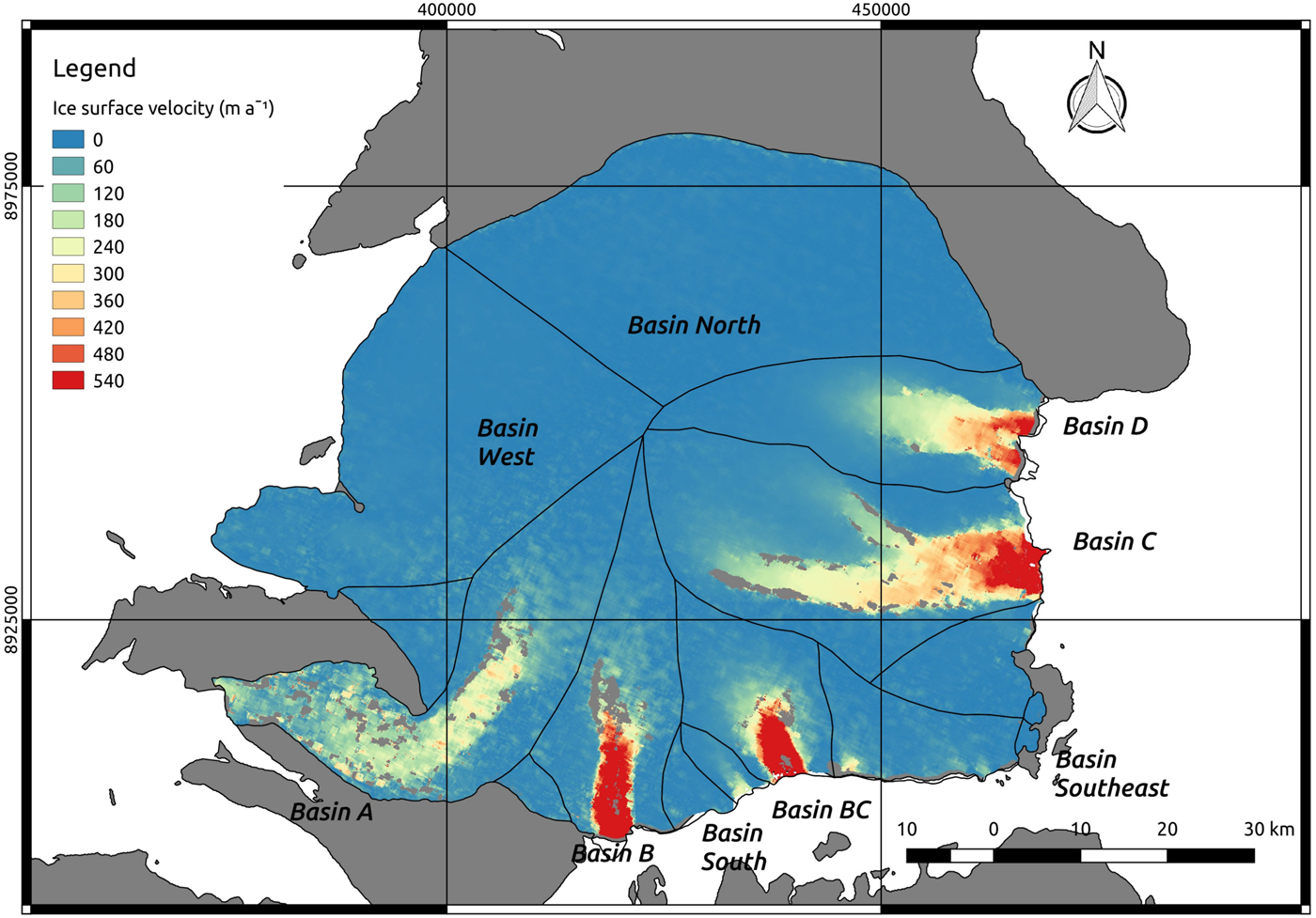
Fig. 2. Surface velocities for the various drainage basins of the Academy of Sciences Ice Cap. Velocities correspond to the Sentinel-1 SAR image pair acquired on 6 and 18 March 2017. Grey colour is used for both ice-free land areas and zones where ice velocities could not be calculated.
The surface-velocity fields of all major ice streams, except A, show a similar pattern. Surface velocity starts to increase where ice flow converges from upper accumulation areas and increases to a maximum at marine glacier termini. Ice Stream A, however, decreases in velocity before the glacier terminus is reached and slightly increases again as the terminus is approached.
In addition to the ice cap-wide surface-velocity field, we computed the mean annual velocities at the flux gates of all marine-terminating basins, which were used to compute the ice discharge. These velocities are shown in Table 1, together with the main characteristics of the corresponding flux gates. The maximum velocity at the flux gate of each of the basins with a well-developed ice stream (A, B, BC, C, D) is also given. We also analysed, during our observation period November 2016–November 2017, the intra-annual variability of surface velocity (both seasonal and shorter-term variations) for the fastest-flowing ice streams (B, BC, C, D). The main results are shown in Figure 3 and Table 2. Ice Stream A is not represented because we did not identify a significant seasonal signal. The velocities shown here are spatially-averaged values over an across-flow window located at the fastest (central) part of each stream, at the flux-gate location. The approximate across-flow averaging-window sizes were: 5 km for Basin B, 7 km for Basin BC and 10 km for Basins C and D. Each graph in Figure 3 consists of 54 velocity values representing 12-d averages. For each of the time series we did a least-squares fit to a model (red line in Fig. 3) consisting in the sum of a straight line (representing a linear trend) and a sinusoidal signal (representing the seasonal variability). The parameters of the fit are given in Table 2. The latter also shows the mean annual velocities (November 2016–November 2017) over the fastest-flowing central parts of Ice Streams B, BC, C and D (the same across-flow windows used in Fig. 3). The seasonality given in the table is the percentage of the amplitude (half of the variation range) of the sinusoidal fit function with respect to the mean annual velocity. The intra-annual velocity variability is also given. This is computed as the percentage of the mean of the absolute values of the velocity deviations with respect to the annual mean velocity (the maximum percentage deviation is also given).
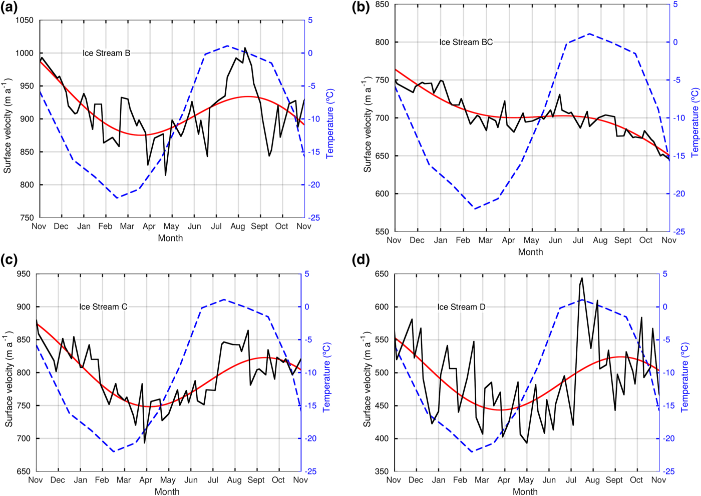
Fig. 3. Temporal variability, during the period November 2016–November 2017, of the surface velocity for the fastest ice streams of the Academy of Sciences Ice Cap, and their fit to a velocity model (red line) consisting of a straight line plus a sinusoidal signal. The dashed blue line is the monthly-averaged air temperature over the ice cap (average value for the three cells of NCEP/NCAR Reanalysis 1 over Northern Komsomolets Island). All panels have a common vertical scale for temperature.
Table 1. Principal characteristics and mean annual (November 2016–November 2017) ice-discharge rates for the marine-terminating drainage basins of the Academy of Sciences Ice Cap shown in Figure 2

Velocity and thickness are average values over each basin's flux gate (FG). Approximate maximum velocities for the main basins are also given. Maximum velocities are not given for the basins without a well-developed ice stream, because they would be not representative of the flow regime
Table 2. Mean annual surface velocities (November 2016–November 2017) over the fastest-flowing central parts of Ice Streams B, BC, C and D, and main parameters of the least-square fit to a velocity model of the temporal variations in velocity shown in Figure 3

The principal parameters characterizing the intra-annual velocity variations are also given. See in the main text the explanation of the various parameters shown in this table.
Note that the velocities presented in Figure 3 do not match exactly those given in Table 1, because the latter are calculated over the entire flux-gate length, whereas the former correspond to a smaller across-flow window at the fastest zone of each ice stream, near the terminus. Excluding Ice Stream BC, which has only weak seasonality (Table 2), the purely seasonal signal (assumed to be given by the sinusoidal fit) is at a minimum in late March and April, and reaches a maximum around mid-September, but slightly earlier (mid-August) for the fastest ice stream (Ice Stream B). The minimum/maximum observed velocities do not always match exactly to the corresponding minima/maxima of the seasonal fits. For Ice Stream B, the minimum observed velocity occurs 1 month later than the minimum of the seasonal fit, and the maximum observed velocities for Ice Streams C and D occur in July–August, ~ 1 − 2 months earlier than the maximum of their seasonal fits, which takes place in mid-September. For IceStreams B, C and D the maximum observed velocities correspond to a period of sustained high velocities lasting for about 2 months in July–August (see Fig. 3).
Ice Streams B, C and D also exhibit short-term, non-seasonal intra-annual variations throughout the year. The velocity variations typically range between 50 and 100 m a−1 but reach up to 200 m a−1 for Ice Stream D, and are therefore markedly above our error estimate of 8.75 m a−1 given in section ‘Ice-surface velocity error estimates’. Ice Stream D is the slowest on the ice cap (mean annual velocity of 491 m a−1) but shows the largest velocity variations, more than 200 m a−1 during the period of sustained high velocities starting in early July (whose peak-to-peak variation represents a ~40% change over the mean annual velocity). By contrast, Ice Stream BC, whose average velocity is relatively high (703 m a−1) shows the smallest intra-annual velocity variations (in addition to the weakest seasonal signal), but has the largest deceleration (− 118 m a−2) during the period under study. Ice Stream B is the fastest (average velocity of 912 m a−1) and has medium-to-large velocity variations. Finally, Ice Stream C has a relatively high average velocity (796 m a−1) and medium-range velocity variations, somewhat lower than those of Ice Stream B. Figure 3 also shows the mean monthly air temperature over the entire Academy of Sciences Ice Cap. Note that the seasonal temperature signal is ~ 1 − 2 months ahead of the purely -seasonal velocity signal, and that the time of the maximum temperatures is coincident with the maximum observed velocities, corresponding to the sustained high-velocity period.
Ice discharge
We estimate a total ice discharge of 1.93 ± 0.12 Gt a−1 from the Academy of Sciences Ice Cap during November 2016–November 2017. Contributions from the individual basins are presented in Table 1. The largest contributors to ice discharge are the southern (B and BC) and eastern (C and D) basins, where the fastest ice streams are located. Drainage Basin BC, which in our case is the third largest contributor to total ice discharge, was not found in previous studies to be a significant source of ice discharge (Dowdeswell and others, Reference Dowdeswell2002; Moholdt and others, Reference Moholdt, Heid, Benham and Dowdeswell2012a). Our data thus indicate that fast ice-stream flow was initiated in this basin after the period covered by the two earlier studies (i.e. after 2009) and before our study period began in 2017. The intra-annual and seasonal variations in ice discharge are associated with corresponding changes in ice velocity. The magnitude of the intra-annual velocity variations thus gives an indication of the error that would be incurred if the ice velocities calculated at a particular snapshot in time were extrapolated to calculate the ice discharge for the whole year. The maximum intra-annual variation in ice discharge at a basin scale (which corresponds to the maximum observed surface-velocity variation during our observation period), is found in Basin C and reaches 0.15 Gt a−1. It is associated with the period of sustained high velocities in July–August (Fig. 3c). Although the velocity variations for this period are larger for Basin D, the ice discharge of Ice Stream C is larger (due to its thicker ice and faster velocity), resulting in a larger ice discharge variation.
Ice cap flow regimes
A map of the pattern of driving stresses on the Academy of Sciences Ice Cap, based on the 2016 ArcticDEM mosaic product, is shown in Figure 4. Noticeable changes (and more detail) can be seen compared to the driving stress map of Dowdeswell and others (Reference Dowdeswell2002). In general terms, the lower resolution of the driving stresses calculated with the airborne altimetric data from the 1997 radio echo-sounding campaign allowed only major patterns over the ice cap to be seen (e.g. the decrease in driving stress on the summit). In Figure 4, the areas of largest driving stress are readily observed in the regions of convergent flow at the heads of the ice streams. The most remarkable examples are Ice Streams D and BC, whose driving stresses reach values of up to 150 kPa at their heads (Fig. 4). Ice Streams A and B show a similar driving stress distribution, but their maximum values are lower, at about 100 kPa (Fig. 4). There are also areas of high driving stress in Basin Southeast, Basin North and along the land-terminating margin of the small (unnamed) basin between Basin A and Basin West, with values of 125, 100 and 100 kPa, respectively.
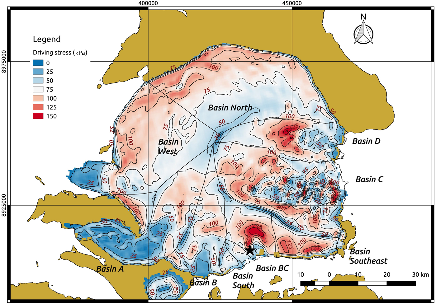
Fig. 4. Driving stress field for the Academy of Sciences Ice Cap. Driving stresses are calculated using ice-thickness data from the 1997 radar campaign and the surface slopes derived from the ArcticDEM mosaic product. The black star shown in the figure indicates the decrease in driving stress between this study and Dowdeswell and others (Reference Dowdeswell2002) (see section ‘Initiation of ice-stream flow at Basin BC’).
The map of flow regimes, derived from the interpretation of surface velocity, ice thickness and driving stress fields, is presented in Figure 5. Table 3 summarizes the main characteristics of each flow regime as defined in section ‘Ice-flow regime mapping’. Flow regime 1 dominates in the slow-moving zones of the ice cap, including Basins North and West, and the upper reaches of all other basins. Flow regime 2 is present in the zones of transition from the low-velocity regions at the upper reaches of the various basins to the high-velocity zones of the ice cap, and coincides with convergent flow at the head of the ice streams (Burgess and others, Reference Burgess, Sharp, Mair, Dowdeswell and Benham2005). In addition, as described by Burgess and others (Reference Burgess, Sharp, Mair, Dowdeswell and Benham2005), flow regime 2 normally shows a transition from a convex-up profile typical of flow regime 1 to a concave-up surface profile. Interestingly, flow regime 3 is only present over a large area at the head of Ice Stream BC and more subtly at Ice Stream D. In the rest of the major drainage basins (i.e. Basins A, B and C), a fast transition from flow regime 2 directly to flow regime 4 occurs. This behaviour suggests a rapid shift from zones of high viscosity and flow resistance to zones of low friction at the glacier bed, which may be linked to the presence of deformable marine sediments beneath the outer part of the ice cap, much of which lies below modern sea level (Dowdeswell and others, Reference Dowdeswell2002). These authors noted that internal deformation alone would account for just a few metres per year of movement, implying that fast flow within the Severnaya Zemlya ice streams is possible to be through basal motion. Given that ~ 50% of the ice-cap bed lies below present sea level and glaciers terminate in the adjacent seas, it is possible that much of the bed is made up of deformable marine sediments.
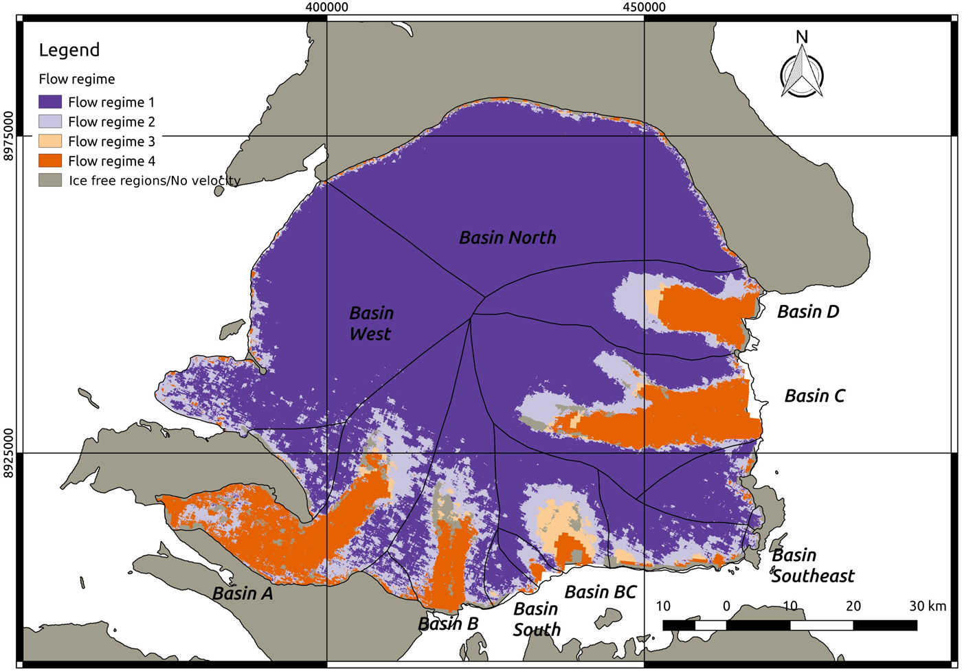
Fig. 5. Flow regimes of the Academy of Sciences Ice Cap (see Table 3 and section ‘Ice-flow regime mapping’ for the description of the flow regimes).
Table 3. Flow regime classes

Surface-elevation changes and associated mass changes
Surface-elevation change rates are shown in Table 4 and Figure 6. The surface-elevation changes at a decadal scale (2004–2016) and at the recent, short-term scale (2012/2013–2016) are similar, except for Basin B. The thinning rate for Basin B during the second period is double than that of the first period. The decadal scale surface-elevation change rate map displayed in Figure 6a shows a general thinning pattern in all marine-terminating basins and a state close to balance on the land-terminating northern and marine-terminating western drainage basins. The thinning is largest for the basins with ice streams draining to the southeast and east (Basins BC, C and D). Note the similarity between the surface-elevation change rates (Fig. 6) and the driving stresses (Fig. 4). The reason for this similarity is that the zones of high slopes and, hence, large driving stresses, are prone to thinning in order to restore the force balance. Drainage Basin A, which has the slowest ice-stream flow, shows only limited average thinning, but greater thinning in its upper reaches and thickening at lower elevations. The thinning pattern is similar for all fast-flowing basins. The highest thinning rates occur where flow converges from the accumulation areas at the heads of the major ice streams (e.g. Basin BC in Fig. 6b).
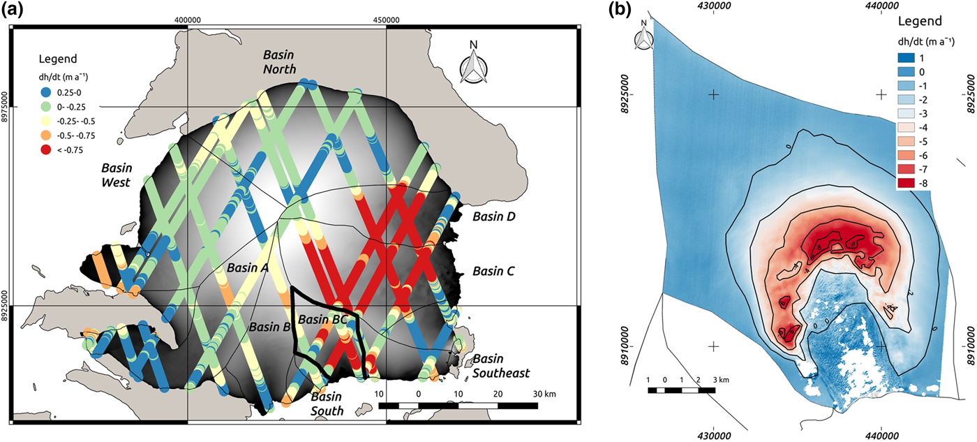
Fig. 6. (a) Results from ICESat-ArcticDEM differencing for the Academy of Sciences Ice Cap in terms of surface-elevation change rates. The background image of the ice cap is the ArcticDEM mosaic product. Basin BC is highlighted. (b) Results from ArcticDEM-ArcticDEM strip differencing for Drainage Basin BC in terms of surface-elevation change rates (from 2012-05-11 to 2016-07-14). White represents no data. Additional results of thinning rates from ArcticDEM-ArcticDEM strip differencing can be found in Supplementary Material Figures S5, S6 and S7 for Basins B, C and D, respectively.
Table 4. Mean annual surface elevation and mass-change rates for the main marine-terminating drainage basins of the Academy of Sciences Ice Cap. Values are calculated from both ICESat-ArcticDEM and ArcticDEM-ArcticDEM differencing, which represent decadal (2004–2016) and recent, shorter-term (2012/13–2016) average values, respectively (see Supplementary Material Table S5)

ICESat elevation changes are extrapolated hypsometrically. The rates for some basins during 2012/13–2016 are not given because of insufficient coverage of the WorldView images in 2012/13. Mass-change rates are calculated assuming an ice density of 900 kg m−3.
Climatic mass balance
As discussed in subsection ‘Climatic mass balance’ of section ‘Methodology', we calculated the climatic mass balance from the total mass balance and the calving flux using Eqn (6). The total mass balance was obtained from surface-elevation changes using the geodetic method. As we aimed to obtain a climatic mass-balance estimate for a period as close as possible to present, we took the geodetic mass balance for the period 2012/13–2016. However, no geodetic mass-balance data were available for certain basins (North, West, South, Southeast) because of the lack of coverage by WorldView images. For these basins, we used instead the geodetic mass balance for the period 2004–2016. This use of a longer-term mass balance is justified because no significant changes were detected in the drainage basins with insufficient WorldView coverage. The results for each basin are found in Supplementary Material Table S4. For the whole ice cap, a total geodetic mass balance $\dot {M} = -1.72\pm 0.67\,{\rm Gt}\,{\rm a}^{-1}$ (− 0.31 ± 0.12 m w.e. a−1) was obtained. If the 2004–2016 rates had been used for all basins, the geodetic mass balance would have been − 1.74 ± 0.67 Gt a−1 (− 0.31 ± 0.12 m w.e. a−1); an insignificant difference. This total mass balance for the ice cap can be divided into a climatic mass balance $\dot {B}= 0.21\pm 0.63\,{\rm Gt}\,{\rm a}^{-1}$
 (0.04 ± 0.12 m w.e. a−1), not significantly different from zero, and a calving flux $\dot {D}= -1.93\pm 0.12\,{\rm Gt}\,{\rm a}^{-1}$
 (− 0.35 ± 0.02 m w.e. a−1). The total mass balance of the ice cap is therefore dominated by the calving flux.
Discussion
Intra-annual and seasonal ice velocity variations
To determine the processes that might drive the observed short-term ice velocity variations (Fig. 3), and in particular whether they respond to an external forcing with a spatial scale large enough to affect all basins (e.g. atmospheric forcing), or are driven by local dynamic conditions which can differ among basins (e.g. surface slope, ice thickness, subglacial bed conditions or topography), it is of interest to analyse whether the changes observed in the various basins are correlated. Only the sustained period of high velocities during July–August is synchronous between all ice streams, except BC, indicating a likely large-scale forcing. Ice Streams C and D show relatively similar variations, although they are much larger in magnitude for D, suggesting external forcing modulated by local dynamic conditions. As all basins show many non-correlated velocity variations, the local dynamic conditions appear to play a role in shaping the observed velocity variations (Fig. 3).
In section ‘Ice cap surface velocity and intra-annual variability’ it was noted that our sinusoidal model of seasonal velocity variations was lagging air temperatures by 1–2 months (Fig. 3). This supports the interpretation that the summer speed-up is triggered by the drainage of surface meltwater to the glacier bed, enhancing lubrication and basal sliding (Zwally, Reference Zwally2002), as has been observed in many Arctic regions (e.g. Dunse and others (Reference Dunse, Schuler, Hagen and Reijmer2012) for Svalbard, and references therein for other Arctic regions). As explained by Copland and others (Reference Copland, Sharp and Nienow2003), glacier acceleration usually lags the onset of summer melt. Meltwater refreezes in the snowpack until the cold content of the snow and firn decreases, thereby causing delayed runoff. Basal lubrication does not occur until a connection between the supraglacial and the englacial/subglacial drainage systems is established.
In our case study from Severnaya Zemlya, maximum observed velocities occurred during the sustained high-velocity period beginning in late June–early July and lasted for almost 2 months (3 months for the fastest ice stream). The sudden drop in velocities following this period, taking place when the air temperatures remain relatively high (monthly average temperature above − 1°C) for 1–2 additional months (and sustained melt is thus expected), suggests that the abrupt slow-down could be due to the transition from a hydraulically inefficient distributed drainage system to an efficient channelized system (Schoof, Reference Schoof2010; Sundal and others, Reference Sundal2011).
The maximum of the seasonal velocity trend (sinusoidal fit in Fig. 3) occurs around mid-September (or mid-August, in the case of Ice Stream B, the fastest ice stream). In 2017, the maximum is nearly coincident with the period when the coasts of northern Severnaya Zemlya are shifting from being nearly sea-ice free to being fully sea-ice covered (Supplementary Material Fig. S1). This is of interest because Zhao and others (Reference Zhao, Ramage, Semmens and Obleitner2014) have shown, by ruling out regional temperature influence using partial correlation analysis, that the total melt days on both Novaya Zemlya and Severnaya Zemlya are statistically anti-correlated with regional late summer sea-ice extent, linking ice and snow-melt on land to regional sea-ice extent variations.
The relationship between higher air temperatures, increased surface melt, and enhanced basal lubrication and sliding can thus potentially explain the seasonal velocity variations. It is also expected to explain the shorter-term intra-annual velocity changes occurring during summer, although the monthly resolution of the temperature data prevents making a stronger argument. However, on the Academy of Sciences Ice Cap intra-annual velocity variations occur throughout the year, not just during summer. This is a common feature of the observed velocities of many outlet glaciers in Greenland and other polar regions (Howat and others, Reference Howat, Box, Ahn, Herrington and McFadden2010; Dunse and others, Reference Dunse, Schuler, Hagen and Reijmer2012) but its occurrence during the winter is seldom analysed in the literature. Attempting to understand the reasons for these observed velocity variations, a Fourier analysis of the residual signal resulting from subtracting the linear trend and the sinusoidal fit from the velocity time series was undertaken. However, the Fourier power spectra did not show any significant peaks, implying that we can discard periodic processes such as monthly tidal variations (note that, because of the 12-d averaging and 7-d sampling period, we cannot detect any shorter-period tidal component). Other possible periodic signals, such as regular passage of cyclones, cannot be detected because of our velocity data resolution, as typical cyclone frequencies over northern Severnaya Zemlya are 0.075−0.1 d−1 (a 10−13 d periodicity) during the winter and 0.125−0.15 d−1 (7–8 d periodicity) during summer (Zahn and others, Reference Zahn, Akperov, Rinke, Feser and Mokhov2018). Other mechanisms that could drive quasi-periodic variations in velocity, such as stick-slip motion (Bindschadler, Reference Bindschadler2003; Sergienko and others, Reference Sergienko, MacAyeal and Bindschadler2009; Winberry and others, Reference Winberry, Anandakrishnan, Alley, Bindschadler and King2009), have a much shorter periodicity (~ 1 d), associated with forcing by daily tides, and thus cannot be tested using the available data.
We checked other theories that could help us to explain the observed velocity variations during the winter. However, we were unable to reach significant conclusions, either because these theories could only explain constant bed deformation or because we lacked additional observational data necessary to test such theories. For completeness, we briefly present these theories in Supplementary Material section ‘Some theories that could explain the velocity variations observed during the winter’.
Initiation of ice-stream flow at Basin BC
The most striking difference in ice-cap dynamics between our study and those of Dowdeswell and others (Reference Dowdeswell2002) and Moholdt and others (Reference Moholdt, Heid, Benham and Dowdeswell2012a) is the initiation of ice-stream flow in Basin BC. This flow accounts for nearly all of the difference in total ice discharge from the ice cap between our own estimate for 2016/2017 (1.93 Gt a−1) and that of Moholdt and others (Reference Moholdt, Heid, Benham and Dowdeswell2012a) for 2003–2009 (1.4 Gt a−1). Ice-stream flow was clearly not visible in the interferograms in Figure 9 of Dowdeswell and others (Reference Dowdeswell2002) or in Figure 5a of Sharov and Tyukavina (Reference Sharov and Tyukavina2009), both based on the SAR acquisitions of 1995. In fact, Dowdeswell and others (Reference Dowdeswell2002) explicitly mention (pp. 5–10) that ‘A fifth basin with rough topography, on the south side of the ice cap, shows only limited evidence of fast flow’. The decrease in driving stress between the study by Dowdeswell and others (Reference Dowdeswell2002) (between 75 and 100 kPa; Fig. 12a of Dowdeswell and others (Reference Dowdeswell2002)) and our analysis (25–50 kPa; black star marks location in Fig. 4), reflects the large drop in surface slope associated with the initiation of stream flow. Additionally, the map of the flow regimes (Fig. 5) reveals a peculiar pattern for Ice Stream BC. The extent of flow regime 3 (see section ‘Ice-flow regime mapping’ and Table 3 for a summary of the flow regimes) for Ice Stream BC is the largest of all the observed ice streams. The size of the zone of combined flow regimes 2 and 3 is also much larger than that of flow regime 4. This suggests a later initiation in time of ice stream flow in this basin as compared with Basins B, C and D. The reason is that zones with well-developed ice stream flow are expected to be dominated by flow regime 4 and to have a shorter zone of transition between flow regimes 1 and 4 (under the assumption of similar soft-bedded sediments in the zones of fast flow). Comparison of a Landsat-7 image of July 2002 with a Sentinel-2 image from March 2016 (Fig. 7) clearly shows the initiation of fast flow. Note the similarity of the flow characteristics of Basin South in both images, in clear contrast with the marked dissimilarity for those of Basin BC, with stream flow evident in the 2016 image. All of the above suggests that stream flow in Basin BC was initiated after 2002, and before 2016.
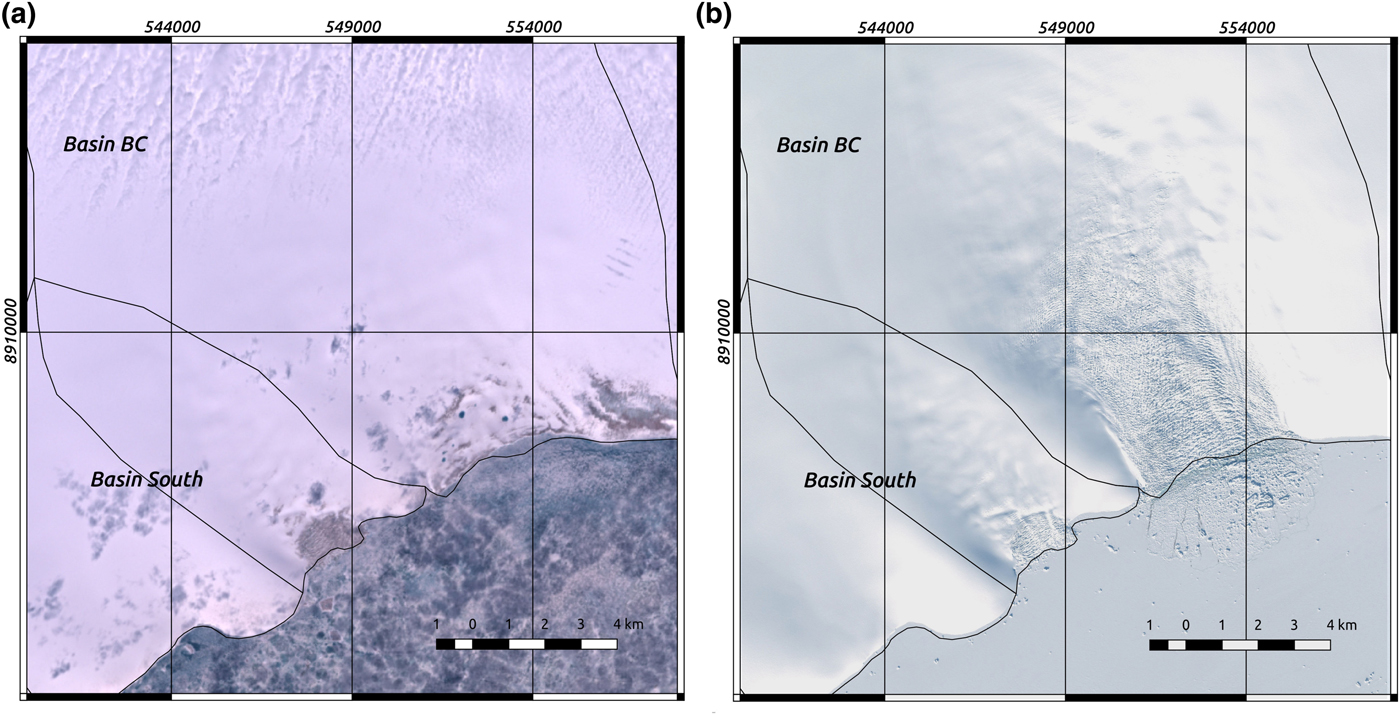
Fig. 7. Comparison of (a) Landsat-7 and (b) Sentinel-2 images, acquired on 09/07/2002 and 29/03/2016 respectively. The crevassing of Ice Stream BC is noticeable on the second image.
Interpretation of surface-elevation changes, calving flux and mass balance between 1988 and 2016
Changes of thinning rates with respect to those of previous studies.
We here discuss, at a basin scale, the main changes in thinning rates between the two periods analysed in more detail by Moholdt and others (Reference Moholdt, Heid, Benham and Dowdeswell2012a) (1988–2006 and 2003–2009) and our own study periods (2004–2016 and 2012/13–2016) (Supplementary Material Table S5, in terms of mass balance). Recall, from section ‘Surface-elevation changes and associated mass changes’, that the changes in thinning rate between the periods 2004–2016 and 2012/13–2016 were negligible, with the exception of Basin B. Also note that our study period 2004–2016 partly overlaps with the period 2003–2009 analysed by Moholdt and others (Reference Moholdt, Heid, Benham and Dowdeswell2012a). Basins North (land-terminating) and West (marine-terminating but with slow flow) are grouped together under ‘North’ in Moholdt and others (Reference Moholdt, Heid, Benham and Dowdeswell2012a) study, and have remained fairly stable along the entire set of periods analysed. Basin A in 2004–2016 shows thinning at its upper elevations and thickening at lower levels, as observed during both periods analysed by Moholdt and others (Reference Moholdt, Heid, Benham and Dowdeswell2012a), who noted a surge-like elevation change pattern supported by the velocity fields of the 1995 InSAR data of Dowdeswell and others (Reference Dowdeswell2002). Moholdt and others (Reference Moholdt, Heid, Benham and Dowdeswell2012a) also noted a decrease in dynamic instability (implying a reduction in ice flow) between 1988–2006 and 2003–2009, indicating glacier deceleration. This trend has continued during our observation period of 2004–2016, with differences in surface-elevation change rates between the upper and lower parts larger than 0.8 m a−1 (Fig. 6a), suggesting continued deceleration.
Surface-elevation change rate decreased in Basin B, from − 1.26 ± 0.31 m a−1 in 1988–2006, to − 0.28 ± 0.11 2004–2016 and to − 0.58 ± 0.18 m a−1 in 2012/13–2016. Moreover, its spatial pattern of surface-elevation changes (Figs 6a and S5) is of particular interest, as it shows a surge-like pattern, with current marked thinning in the upper part of the basin (~ −2 m a−1) and thickening in the lower part of the ice stream (~ 1 m a−1).
Basins South, BC and Southeast are reported jointly under ‘Others’ in the study by Moholdt and others (Reference Moholdt, Heid, Benham and Dowdeswell2012a). They showed a transition from a near-balance value of − 0.02 ± 0.10 m a−1 in Moholdt and others (Reference Moholdt, Heid, Benham and Dowdeswell2012a) for 2003–2006 to thinning in the 2004–2016 period (surface-elevation change rate of − 0.59 ± 0.17 m a−1). This transition is more marked if Basin BC is considered separately, as it showed a rate of − 1.31 ± 0.33 m a−1 for 2004–2016, due to the initiation of ice stream flow.
Basin C experienced widespread thinning during all periods, but the change was more marked during the earliest interval, with average surface-elevation change rates of − 2.56 ± 0.26 m a−1 in 1988–2006, changing to ~ −1 m a−1 in the two most recent periods (Fig. S6 and, in terms of mass balance, Table S5). Basin D has also shown widespread thinning in all periods, but decreasing slowly in magnitude through time. This indicates sustained fast flow and large cumulative thinning (Fig. S7).
These changes in surface elevation indicate a larger dynamic thinning and a larger contribution to mass loss by the marine-terminating southern and eastern drainage basins for 2004–2016 and for 2012/13–2016, as compared with the results of Moholdt and others (Reference Moholdt, Heid, Benham and Dowdeswell2012a) for 2003–2006. This largest thinning, at the zones of onset of ice-stream flow, is an additional indication of dynamic instability.
Comparison of calving fluxes with previous studies.
Calving flux estimates for the Academy of Sciences Ice Cap, derived using different techniques, are available for various periods (some of them overlapping) within the last ~30 years. Dowdeswell and others (Reference Dowdeswell2002) estimated the calving flux for September/December 1995 using SAR interferometry, whereas Moholdt and others (Reference Moholdt, Heid, Benham and Dowdeswell2012a) calculated flux for the period June 2000–August 2002 using image-matching of Landsat scenes. For the periods 1988–2006 and 2003–2009, Moholdt and others (Reference Moholdt, Heid, Benham and Dowdeswell2012a) estimated the ice discharge in an indirect way, subtracting from the geodetic mass balance (calculated from DEM differencing assuming Sorge's law) an estimate of the climatic mass balance. The latter was based on the assumption (which we have also made in our total mass balance estimate discussed in section ‘Total ablation by surface and frontal loss') of considering Basin North (basins North and West in our study) as an analogue for the climatic mass balance of the whole ice cap (Moholdt and others, Reference Moholdt, Heid, Benham and Dowdeswell2012a). This assumption was justified because the northern part of the ice cap is land-terminating (and thus climatic mass balance and geodetic mass balance are equal) and its western part, although marine-terminating, appears to be dynamically inactive with no significant calving losses. Extrapolating the estimated climatic mass balance to the rest of the ice cap leads to a near-zero climatic mass balance for the whole Academy of Sciences Ice Cap, which is consistent with other pieces of evidence that will be discussed later.
All available calving flux results are shown in Table 5. Significant variations are evident during the entire period, although the calving flux in the last decade seems to have been more stable than in previous decades (Table 5). Note that the difference of ~ 0.5 Gt a−1 between the estimates for 2003–2009 and 2016–2017 can be almost entirely attributed to the recent initiation of fast flow in Basin BC (section ‘Initiation of ice-stream flow at Basin BC’ and Table 5, included in ‘Others’). The lowest calving flux estimate (0.6 Gt for 1995) used a DEM of limited accuracy, derived from an airborne pressure-based altimeter (Dowdeswell and others, Reference Dowdeswell2002). This implies large uncertainties in the estimated calving flux. Additionally, as pointed out by Moholdt and others (Reference Moholdt, Heid, Benham and Dowdeswell2012a), in the study by Dowdeswell and others (Reference Dowdeswell2002) ice velocity could only be detected in the satellite look direction (northeastward), leading to a likely underestimate. Moreover, note that in Dowdeswell and others (Reference Dowdeswell2002) work ice velocity for Ice Streams B, C and D was not resolved (phase coherence broke down) near the margins, so the closest point of velocity evaluation was ~ 5 − 8 km from the calving front. This implies that the highest velocities further down-glacier were not used in the discharge estimate, leading to a likely underestimate (in our study, this distance is of ~ 1.5 − 3 km from the terminus, just enough to avoid any possible floating tongues).
Table 5. Estimated calving flux for the drainage basins of the Academy of Sciences Ice Cap for various periods. Basin North here groups Basins North and West, and ‘Others’ groups Basins South, BC and Southeast

These names are used for compatibility with Moholdt and others (Reference Moholdt, Heid, Benham and Dowdeswell2012a)
The main potential shortcoming of the indirect estimates of calving flux for 1988–2006 and 2003–2009 is the assumption of Sorge's law in the conversion from volume changes to mass changes (i.e. that there is no changing firn thickness or density through time). The amount of melt layers in ice cores is a proxy for the summer warmth at the ice-cap surface (Koerner, Reference Koerner1977). In the analysis by Opel and others (Reference Opel2009) of the deep ice core taken in 1999–2001 at the summit of Academy of Sciences Ice Cap, a strong increase in melt-layer content was found at the beginning of the 20th century, which remained at a high level until about 1970 and then decreased markedly until 1998. These large temporal variations in melt-layer content, together with modelling experiments on the neighbouring Vavilov Ice Cap on October Revolution Island (Bassford and others, Reference Bassford, Siegert and Dowdeswell2006a,Reference Bassfordc), Severnaya Zemlya, indicate that the assumption of an absence of temporal change in firn thickness or density is not suitable for the Academy of Sciences Ice Cap. Even so, the associated uncertainty cannot justify the large differences in calving flux observed between the various periods shown in Table 5. In the case of the calving flux estimates based on data for particular snapshots in time, the period (within the year) when the observations were made can neither explain such large differences, on the light of the magnitude of the seasonal and intra-annual variability in surface velocities analysed in earlier sections. Consequently, there is a need to search for drivers of the large differences in calving flux observed over the last three decades.
Drivers of observed long-term changes in calving flux.
Increasing summer air temperature may be a driver of increasing calving, through its influence on surface melting followed by drainage to the glacier bed, enhancing bed lubrication and basal sliding (Zwally, Reference Zwally2002). However, such accelerations in velocity are mostly short-lived and do not contribute to increased calving (Sundal and others, Reference Sundal2011). Air temperatures could still play a role if they had an influence on sea-ice or ice mélange concentration, as these are known to affect calving, especially when glaciers are confined in fjords (Moon and others, Reference Moon, Joughin and Smith2015; Otero and others, Reference Otero2017). However, the possible effects of sea-ice cover on the dynamics and calving flux of the Academy of Sciences Ice Cap are expected to be weak, as their marine termini are not confined in fjords where sea ice or ice mélange could form, be retained and exert a significant backpressure. Moreover, the seas surrounding Severnaya Zemlya are characterized by relatively thin first-year ice, because this is a region where new ice is produced and soon moved away by the oceanic currents that flow northwards past the archipelago and subsequently turn to the west towards Fram Strait (Serreze and Barry, Reference Serreze and Barry2014). However, Sharov and Tyukavina (Reference Sharov and Tyukavina2009) pointed out that medium-term (from decadal to semi-centennial) changes in glacier volumes on Severnaya Zemlya were linked to the extent and duration of sea-ice cover nearby, so that slow-moving maritime ice caps would grow when the sea-ice cover in adjacent waters was small, and thin when the sea-ice cover consolidated. This, however, would apply in our case study only to the slow-moving Basins West and A. More generally we did not find any clear relationship between summer (June–July–August) average temperature and calving flux, or between sea-ice concentration and calving flux, which could explain the observed long-term changes in calving flux (Figs S2, S3). In fact, the highest calving fluxes corresponded to the period 1988–2006, which had, overall, lower air temperatures and larger late September sea-ice extent than the periods 2003–2009 and 2016–2017 (Figs S2, S3). The calving flux in 2003–2009 was lower than that of 2016–2017, and mean summer temperatures during 2003–2009 (~ 0.8°C on average) were higher than that of summer 2017 (− 0.2°C). The mean late September sea-ice extent was also higher on average for 2003–2009 compared with 2016–2017 (Fig. S2). Only for the lowest calving flux estimate, which corresponds to particular snapshots in time (September and November 1995), did we find that the sea-ice extent in late September was larger than those of the preceding and following years (Fig. S2). The summer before our SAR image acquisitions (2016) was relatively warm (mean summer air temperature of 1.2°C), but was followed by a marked drop in temperature, to − 0.2°C in summer 2017 (Fig. S3). However, the sea surrounding northern Severnaya Zemlya was virtually ice free at the end of September 2017 (Fig. S1).
In the absence of a clear climate-related driver for the large interannual changes in calving flux observed during the last three decades, we are inclined to associate the observed dynamic instabilities with intrinsic characteristics within the Academy of Sciences Ice Cap, as suggested by Moholdt and others (Reference Moholdt, Heid, Benham and Dowdeswell2012a). One of the characteristics that could influence long-term variations in terminus position and calving fluxes is the complex geometry of the subglacial and seabed topography in the terminal zones of the eastern basins (C and D) (Dowdeswell and others, Reference Dowdeswell2002). The variations of flux could be associated with changes in floatation conditions (Howat and others, Reference Howat, Joughin and Scambos2007). The floating or near-floating state of these marginal zones has been suggested through various lines of evidence, such as the very low ice-surface gradients, the strong radar returns from the ice-cap bed in several areas at the margin of the ice streams, and the large numbers of tabular icebergs observed near their margins (Dowdeswell and others, Reference Dowdeswell2002).
Comparison of mass-balance rates with previous studies.
The estimates of the total mass balance of the Academy of Sciences Ice Cap within the last three decades are summarized in Table 6. Detail by basin is found in Table S5. All mass balances were obtained by the geodetic method, which has the limitations derived from the use of Sorge's law, discussed earlier. Possible changes in ice-cap area, if significant, would be a further limitation. Dowdeswell and others (Reference Dowdeswell2002) reported an ice-cap area of 5575 km2, based on Landsat images acquired in 1988. Moholdt and others (Reference Moholdt, Heid, Benham and Dowdeswell2012a), using multitemporal satellite imagery from Corona and Landsat acquired between 1962 and 2010, concluded that there have been no clear trends in the terminus fluctuations of the Academy of Sciences Ice Cap, and calculated a total marine-terminating glacier area loss of 5 km2 between 1988 and 2009, which included several examples of local advance and retreat. Their estimated rate of ice-volume loss between 1988 and 2009, due to retreat, was only 0.02 km3 a−1, which is not significant in terms of ice-cap mass balance. Our own observations, using Landsat-7 and Sentinel-2 optical images from July 2002 and March 2016, respectively, showed local advances and retreats of the eastern and southern marine margins of up to ~ 1 − 2 km with respect to the margins of Moholdt and others (Reference Moholdt, Heid, Benham and Dowdeswell2012a), but the net change in area is negligible and thus we have used the same ice-cap area of 5570 km2 of Moholdt and others (Reference Moholdt, Heid, Benham and Dowdeswell2012a).
Table 6. Total mass balance of the Academy of Sciences Ice Cap for different periods. For calculating the values under ‘This study’, for the basins without an estimate for 2012/13–2016, our estimate for 2004–2016 has been taken

The total mass balances shown in Table 6 parallel (with reversed sign) those of the calving fluxes presented in Table 5. The largest difference between the data in both tables (~ 0.3 − 0.4 Gt a−1, for the period 2003–2009), is due to the use by Moholdt and others (Reference Moholdt, Wouters and Gardner2012b) of Basin North as an analogue for the climatic mass balance of the whole ice cap (the slightly positive climatic mass balance of Basin North multiplied by the area of the whole ice cap accounts for this difference). The second largest difference corresponds to the most recent period, and it could be attributed to the fact that the periods considered in both tables are close but not equal (2016/17 vs 2012/13–2016) and, additionally, the mass balances given for certain basins for 2012/13–2016 actually correspond to the period 2004–2016 (as shown in Supplementary Material Table S5), due to unavailability of WordView strips for those basins during 2012/13–2016. Overall, the results in Tables 5 and 6 indicate that the total mass balance of the ice cap is nearly equivalent to the calving losses, which means that the long-term climatic mass balance has remained close to zero since 1988.
The limited earlier observations of climatic mass balance available, for the Vavilov Ice Cap on October Revolution Island some 120 km to the south, also indicate a near-zero average balance of − 0.03 m a−1 for the periods 1975–1981 and 1986–1988 (Barkov and others, Reference Barkov1992), and a similar value of − 0.02 m a−1 for the complete period 1974–1988 from mass-balance modelling experiments (Bassford and others, Reference Bassford2006c). Although all these estimates pointed to large interannual variability, such year-to-year variations have limited interest in the context of this discussion, since we only have average mass-balance estimates over periods of several years, up to more than a decade. We may thus consider that the climatic mass balance of the Academy of Sciences Ice Cap has been close to zero on average during at least the last four decades.
A discussion of the factors that might control long-term changes and trends in mass balance and, in particular, of the climatic mass balance, can be found in Supplementary Material section ‘Possible factors controlling long-term changes and trends in climatic mass balance’. The conclusion is that the long-term near-equilibrium climatic mass balance of the Academy of Sciences Ice Cap (and Servernaya Zemlya ice masses in general) may be the result of two opposing effects. On one hand, low sea-ice cover would enhance precipitation by exposing larger areas of open water to evaporation. On the other, these larger areas of open water would allow onshore advection of heat from warming mixed ocean layers, accelerating surface melt on the ice cap. With the climatic mass balance remaining near zero, the role of the calving flux is critical in determining the total mass balance of the Academy of Sciences Ice Cap.
Total ablation by surface and frontal loss
Having in mind projections of the future contributions of glacier wastage to sea-level rise, we want to know the relative contributions of surface versus frontal ablation to total ablation. Frontal ablation is equivalent, in our case study, to calving flux, which has been calculated before, but the other term, surface ablation, is unknown. To estimate surface ablation, we subtract from our calculated climatic mass balance for 2012–2016 (0.21 ± 0.30 Gt a−1; see section ‘Climatic mass balance’ ) an estimate of total accumulation over the ice cap. Total accumulation is based on the measured net accumulation at the ice-cap summit and its variation with altitude (Dowdeswell and others, Reference Dowdeswell2002).
Various ice core and structural-stratigraphic studies at the ice-cap summit (Fritzsche and others, Reference Fritzsche2002, Reference Fritzsche2005) yielded accumulation values of 0.43–0.53 m w.e. a−1 for several periods between 1963 and 1999 (Supplementary Material section ‘On the calculation of the shares of total ablation by frontal ablation and surface ablation’). Measurements elsewhere in Severnaya Zemlya suggest that annual precipitation decreases with altitude from 0.45 to 0.25 m w.e. a−1 (Bryazgin and Yunak, Reference Bryazgin and Yunak1988). Assuming, as in Dowdeswell and others (Reference Dowdeswell2002), a value of 0.30 m w.e. a−1 as the average accumulation over the entire ice cap, we obtain a total accumulation of 1.67 Gt a−1. Taking account of our positive climatic mass-balance estimate of 0.21 ± 0.30 Gt a−1, the surface ablation will thus be − 1.46 Gt a−1. Added to the frontal ablation of − 1.72 Gt a−1, we derive a total ablation of − 3.18 Gt a−1. This implies that frontal ablation represents, on average, ~54% of the mass losses over 2012–2016, with the remaining 46% corresponding to surface ablation. If we had considered, instead, the upper bound for the accumulation rate of 0.46 m w.e. a−1 (Fritzsche and others, Reference Fritzsche2005), frontal ablation would have represented ~42% of the total ablation over the period 2012–2016, with the remaining ~58% corresponding to surface ablation. We conclude that calving losses are a substantial component, in fact about half of the total mass loss from the Academy of Sciences Ice Cap.
Conclusions
The following main conclusions are drawn from our analysis:
(1) During the period November 2016–November 2017, the marine-terminating margins of the Academy of Sciences Ice Cap remained nearly stable, so that ice discharge and calving flux are equivalent in our study, at 1.93 ± 0.12 Gt a−1. The difference with the estimate by Moholdt and others (Reference Moholdt, Heid, Benham and Dowdeswell2012a) of ~ 1.4 Gt a−1 for 2003–2009 can be attributed to the initiation of ice stream flow in Basin BC after 2002.
(2) The long-term (interannual/interdecadal) variations of ice discharge during the last three decades were large, at between 0.6 and 3.2 Gt a−1. The lack of clear environmental drivers for the observed changes suggests that this dynamic instability is associated with intrinsic characteristics of the ice cap. We suggest that this instability could be caused by the long-term changes in floatation conditions associated with the complex geometry of the subglacial and seabed topography in the terminal zones of the fast-flowing eastern basins (B and C).
(3) The purely seasonal variability in ice velocity (and correspondingly in ice discharge) during the period November 2016–November 2017 is up to ~ 10% of the yearly averaged velocity values (20% peak-to-peak), but the intra-annual variability, considering changes other than seasonal, has average values of up to 16%, depending on basin, but with maximum values of up to 32% of the yearly-averaged velocities (32 and 64% peak-to-peak). This gives an idea of the errors that could be incurred if the ice discharges calculated for particular snapshots in time were extrapolated to mean annual values.
(4) Intra-annual variations in ice velocity during the summer are probably associated with the periods of surface melting, the routing of this meltwater to the glacier bed and enhanced basal sliding. Maximum velocities are reached during a sustained high-velocity period lasting for about 2 months and followed by an abrupt slow-down in velocities well before the end of the melt season. This abrupt drop in velocities may be due to the transition from a hydraulically inefficient distributed drainage system to an efficient channelized system. An explanation for the short-term intra-annual velocity variations observed during winter remains elusive, however.
(5) The average total geodetic mass balance of the ice cap during 2012–2016 was − 1.72 ± 0.27 Gt a−1, equivalent to − 0.31 ± 0.05 m w.e. a−1 over the whole ice cap. The average climatic mass balance of the ice cap during 2012–2016 (similar to that for 2004–2016), was not significantly different from zero, at 0.21 ± 0.30 Gt a−1, or equivalently 0.04 ± 0.05 m w.e. a−1. This is in line with the scarce in-situ observations in the region during the 1970s and 1980s and with remote-sensing estimates by other authors for 1988–2006 and 2003–2009. The average climatic mass balance has thus remained around zero during the last four decades, and the total mass balance has therefore been governed by the calving flux.
(6) We estimate that the average total ablation (surface ablation plus frontal ablation) over the period 2012–2016 was about − 3.18 Gt a−1, of which frontal ablation (mostly calving) represented ~54% and the remaining ~46% corresponded to surface ablation. Calving losses were, therefore, an important contributor to the mass losses from the Academy of Sciences Ice Cap.
Summarising, with a climatic mass balance averaging to zero over the last four decades, in spite of regional warming, the total mass balance of the ice cap has been driven mainly by ice discharge, which does not seem to have responded to environmental changes but instead to intrinsic characteristics of the ice cap such as the subglacial and seabed topography near the marine-terminating margins.
Supplementary material
The supplementary material for this article can be found at https://doi.org/10.1017/jog.2019.58
Acknowledgments
This study has received funding from the European Union's Horizon 2020 research and innovation programme under grant agreement No 727890 and from grants CTM2014-56473-R and CTM2017-84441-R of the Spanish National Plan for R $\&$ D. The radio-echo sounding campaign was funded by grants GR3/9958 and GST/02/2195 to JAD from the UK Natural Environment Research Council. Support to AG by the Russian Fund for basicresearch grant 18-05-60109 is also acknowledged. This research has been carried out as part of the Network on Arctic Glaciology of the International Arctic Science Committee (IASC-NAG). DEMs were provided by the Polar Geospatial Center under NSF OPP awards 1043681, 1559691 and 1542736. Copernicus Sentinel data 2016–2017 were processed by ESA. NCEP reanalysis data were provided by the NOAA/OAR/ESRL PSD, Boulder, Colorado, USA, from their website at https://www.esrl.noaa.gov/psd/. We thank the scientific editor, Beata Csatho, and two anonymous reviewers, for their many suggestions to improve the manuscript.


 Open access