


Impact Statement
What effect does buoyancy have on pollution dispersion behind a backward-facing step? The answer to this question has wide-ranging applications, such as smoke trapped behind a burning building or dispersion of buoyant pollutants in wide street canyons.
With a growing global urban population, we are increasingly situated in close proximity to a multitude of sources of harmful airborne pollution with numerous documented health implications. Understanding and quantifying the mechanisms that transport these, often buoyant, pollutants can help to understand and reduce human exposure. At the low flow speeds associated with urban environments, the effects of buoyancy can be significant. We find here that the concentration of a pollutant trapped in the wake of a building is reduced if that pollutant is positively buoyant. We present a model to predict this reduction in concentration.
1. Introduction
The backwards-facing step is a canonical wake flow that appears in many scenarios ranging from street canyons to aspects of aerofoil design (Reference Mishriky and WalshMishriky & Walsh, 2016). Here, we investigate the effect of buoyancy on pollution dispersion in the wake. Some examples of practical interest include trapping of smoke behind a burning building and dispersal of pollution within street canyons (Reference Simoens, Ayrault and WallaceSimoens, Ayrault, & Wallace, 2007). The backward-facing step also represents a simple model to investigate the effect of buoyancy on wakes more generally, and as such could provide insights into vehicle pollutant dispersion.
The turbulent wake structure of the backward-facing step has several important features (figure 1a). As the free-stream flow passes over the step, a shear layer forms. The shear layer encompasses a recirculation region of low-speed flow located behind the step and eventually reattaches to the ground. Many studies, such as those by Reference Adams and JohnstonAdams and Johnston (1988) and Reference Tihon, Pěnkavovà, Havlica and ŠimčikTihon, Pěnkavovà, Havlica, and Šimčik (2012), have investigated how  $L_r$, the reattachment length, changes with Reynolds number ( $Re_H = UH/\nu$) and expansion ratio ( $E_r = (H+h)/h$; see figure 1a). As found by Reference Nadge and GovardhanNadge and Govardhan (2014), $L_r$ increases with both $E_r$ and $Re_H$, levelling off as the flow becomes Reynolds invariant, at a value of $Re_H$ which depends on the value of $E_r$. The free-stream turbulence levels also affect the reattachment length, as does the thickness of the boundary layer when it separates over the step (Reference Chen, Asai, Nonomura, Guannan and LiuChen, Asai, Nonomura, Guannan, & Liu, 2018).
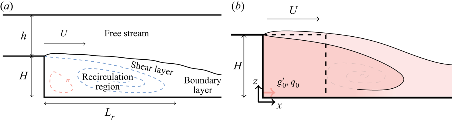
Figure 1. The backward-facing step. (a) Flow structure. A shear layer forms where the flow separates at the top of the step, reattaching to the ground some distance  $L_r$ behind the step. After reattachment the wake structure feeds into a boundary layer. Two vortical structures form in the recirculation region: a larger primary vortex (blue) and a smaller secondary vortex (red). (b) Problem set-up. Step height $H$, free-stream flow speed $U$ and a buoyancy flux per unit depth of $f_{0} = g'_{0} q_0$, where $g'_{0}$ and $q_0$ are the exhaust buoyancy and volume flux per unit depth. Dashed lines indicate an $H \times H$ box over which the concentration will be averaged, allowing comparison of theory with experiments.
At sufficiently high Reynolds number, a separated recirculation region forms behind the step that contains two counter-rotating vortical structures (Reference Chen, Asai, Nonomura, Guannan and LiuChen et al., 2018). The primary recirculation (figure 1a, blue) is the larger of the two and is driven by the shear layer, with the top half of the primary recirculation forming part of the shear layer whilst the bottom half forms the lower bounding velocity for the shear layer. The smaller secondary recirculation (figure 1a, red) is located at the base of the wall of the step and driven by the primary recirculation region. Reference Chen, Asai, Nonomura, Guannan and LiuChen et al. (2018) provide a more extensive review of the flow structure behind the backward-facing step.
Significantly fewer papers have investigated the influence of buoyancy upon the wake of the backward-facing step. Existing research has focused on the case where the step is rotated at right angles to that shown in figure 1(a). A downstream ‘floor’ is uniformly heated and flow is in the vertical direction such that buoyancy either directly assists or opposes the wake (Reference Abu-Mulaweh, Armaly and ChenAbu-Mulaweh, Armaly, & Chen, 1993; Reference Iwai, Nakabe, Suzuki and MatsubaraIwai, Nakabe, Suzuki, & Matsubara, 1999; Reference Niemann and FröhlichNiemann & Fröhlich, 2016). This research has shown that when the buoyancy force aligns with the direction of flow, buoyancy reduces the wake size, while when buoyancy opposes the flow the wake size increases.
There has been some initial research into the effect of buoyancy released into the near wake of a floor-mounted cube (e.g. Reference Lin, Ooka, Kikumoto, Sato and AraiLin, Ooka, Kikumoto, Sato, & Arai, 2020; Reference Olvera, Choudhuri and LiOlvera, Choudhuri, & Li, 2008; Reference Tominaga and StathopoulosTominaga & Stathopoulos, 2018). Those authors have investigated the effect of pollutant source location and the effect of additional cubes up- and downstream. So far, this research has been largely qualitative, has not examined a wide range of buoyancy fluxes or explained the physical mechanisms behind the changes observed in pollution dispersion. Experiments performed within a wind tunnel by Reference Olvera, Choudhuri and LiOlvera et al. (2008) found that increasing the buoyancy of the pollutant moves the concentration and velocity wake profiles upwards. This phenomenon was still significant at five cube heights downstream. Using an ‘origin correction’ method Reference Robins and ApsleyRobins and Apsley (2018) introduced buoyancy into their Gaussian plume model of pollution dispersion behind buildings; however, their model focuses upon far-field pollutant concentrations rather than the near field examined in this investigation.
We systematically examine the effect of buoyancy on pollutant dispersion directly behind the step, for a range of free-stream flow speeds, exhaust buoyancies and exhaust fluxes and develop a model that describes the observations. We outline the problem in § 2 and present some dimensional reasoning, alongside a model that predicts the total pollutant concentration trapped in an  $H \times H$ region behind the step. Section 3 outlines the experimental methods, while § 4 details and discusses the experimental results. We demonstrate that increasing the buoyancy of the pollutant behind the step or decreasing the flow velocity leads to a reduction in the average concentration trapped there. We conclude in § 5.
2. Problem outline and theory
In this section, we outline the problem and the relevant non-dimensional parameters. The relevant variables are illustrated in figure 1(b). There are six dimensional parameters in the problem that can be controlled independently: the free-stream velocity  $U$, the step height $H$, the viscosity of the working fluid $\nu$, the exhaust concentration volume flux $c_0 q_0$ and the exhaust volumetric as well as buoyancy flux per unit depth, $q_0$ and $f_0= q_0g'_0$, respectively. Thereby, $g'_0=g(\rho _0-\rho )/\rho$ is the reduced gravity of the exhaust, $g$ is the gravitational constant, $\rho _0$ and $\rho$ are the densities of the exhaust and the free stream, respectively, and $c_0$ is the concentration of the exhaust.
The units in the problem are time, length and a measure unit for the pollutant concentration. We choose the free-stream velocity  $U$, the step height $H$ as well as the concentration volume flux per unit depth $c_0q_0$ as the repeating variables. The remaining three dimensional parameters can be non-dimensionalised and we form three dimensionless groups: the step Reynolds number, an adapted densimetric Froude number and a dimensionless flow rate analogous to an exhaust dilution rate:
 \begin{equation} Re_H = \frac{UH}{\nu},\quad Fr' = \frac{U}{f_0^{1/3}},\quad \hat{q}_{0} = \frac{q_0}{UH}. \end{equation}
As found by Reference Armaly, Durst, Pereira and SchönungArmaly, Durst, Pereira, and Schönung (1983) and others, at a high enough Reynolds number, the flow around the step becomes Reynolds invariant, which is discussed further in § 3. Furthermore, our experiments have been designed such that  $\hat {q}_{0}$ is small. This is outlined in more detail in Appendix B.2 and discussed further in § 4. Performing our experiments in the Reynolds-invariant regime, and considering $\hat {q}_{0}\approx 0$, allows the collected experimental results to be scaled purely in relation to the adapted Froude number $Fr'$. The upstream flow has been laminarised using two layers of flow-aligning mesh and foam, and as such the turbulence generated within the wake is considered to be much larger than that of the free-stream flow. Hence, the results presented may not be directly applicable to scenarios with considerably turbulent free-stream flows. Reference Caton, Britter and DalzielCaton, Britter, and Dalziel (2003) investigated and modelled dispersion mechanisms in a street canyon for high and low levels of external turbulence. Furthermore, the scenario is considered to have a small boundary layer upon the step. Reference Essel and TachieEssel and Tachie (2015) investigated surface roughness upon the upstream boundary layer and how that changes the shape of the wake, producing nominal changes for the purpose of this investigation.
The adapted Froude number  $Fr'$ is analogous to a densitometric Froude number $Fr$ in that it relates inertial forces to buoyancy. A traditional densitometric Froude number ( $Fr = U/\sqrt {g'_0H}$) can be found through inspection to be $Fr^2 = Fr'^3\hat {q}_0$, and does not constitute a separate non-dimensional group. Since the exhaust is quickly diluted and mixed into the wake, the total buoyancy flux into the wake is more dynamically significant than the exhaust buoyancy strength and therefore $Fr'$ was selected over $Fr$. As we see later, $Fr'$ can also be considered as a ratio of the time scale associated with recirculation in the wake and the time scale associated with buoyancy-driven transport within the exhaust plume.
Similarly, the dynamically significant quantity when non-dimensionalising the concentration downstream of the step is not the concentration of the exhaust  $c_0$, but the concentration volume flux $c_0 q_0$. Therefore, a generic concentration ( $c_{*}$) is non-dimensionalised with the selected repeating variables as
 \begin{equation} \hat{c}_{ * } = \frac{c_{ * }UH}{c_0q_0} = \frac{c_{ * }}{c_0 \hat{q}_0}. \end{equation}
We characterise the concentration behind the step using the average concentration  $\bar {c}_{H\times H}$ in an $H \times H$ square immediately downstream of the step (figure 1b). When non-dimensionalised in accordance with (2.2), this averaged quantity is denoted as $\hat {c}$, such that
 \begin{equation} \hat{c} = \frac{\bar{c}_{H\times H}}{c_0\hat{q}_0}. \end{equation}
We have chosen this measure  $\bar {c}_{H\times H}$ as it can be clearly and objectively defined, i.e. it does not depend on the exact size or shape of the wake.
Invoking Buckingham's  $\pi$-Theorem, we expect the functional relationship
 \begin{equation} \hat{c} = f\left(Re_H, \hat{q}_0, Fr'\right)\approx f(Fr'), \end{equation}
since we consider the Reynolds-invariant regime and the assumption that  $\hat {q}_0\approx 0$, except where it constitutes exhaust concentration flux, since the exhaust concentration is expected to be significantly higher than the average wake concentrations.
2.1 Modelling neutrally buoyant pollution dispersion
We begin modelling our flow by considering the neutrally buoyant case. We time-average the wake and simplify the system into three distinct regions: a well-mixed recirculation region, a shear layer and a free-stream flow (figure 1a). The fluxes of concentration between these three regions are modelled and balanced to estimate the average concentration within the recirculation region  $c_r$. The shear layer and the recirculation vortex are coupled flow structures, with the shear layer driving the recirculation vortex and the vortex feeding into and drawing from the shear layer. From this point onward, the wake of the backward-facing step is separated into a structure resembling a shear layer bounding a low-velocity region below, referred to as the recirculation region.
The shear layer entrains fluid from the recirculation region and the free-stream flow. We parametrise the shear layer with a streamwise coordinate  $s$. In the following, we neglect the effects of curvature of $s$ on the entrainment and detrainment flows of the shear layer. At some point along $s$, the shear layer flow is drawn back (detrained) into the recirculation region. This point of entrainment reversal aligns with the centre of the primary vortex. We define this length along $s$ until this entrainment reversal as $s_1$, and the distance from this point to the end of the shear layer as $s_2$ (figure 2). A careful inspection of our particle image velocimetry (PIV) velocity field measurements (figure 5) shows that the centre of the primary vortex aligns with the midpoint along the shear layer. This has motivated the modelling assumption
 \begin{equation} s_1 = s_2. \end{equation}
We model the entrainment velocity  $U_e$ into the shear layer as being of constant magnitude and proportional to the velocity difference between the midstream velocity and the free stream ${\rm \Delta} U\approx U/2$. This allows the entrainment velocity to be expressed as
 \begin{gather} U_e = E \frac{U}{2}, \end{gather}
 \begin{gather}\hat{U}_e = \frac{U_e}{U} = \frac{E}{2}, \end{gather}
where  $E$ is a constant entrainment coefficient, relating the entrainment velocity to the characteristic velocity deficit between the shear layer and the outside flow. Integrating this velocity over the length $s_1$ gives the total flux $U_es_1$ across the surface. By considering conservation of volume within the recirculation region and using our modelling assumptions $\hat {q_0}\approx 0$ and $s_1=s_2$, we can conclude that the detrainment velocity $U_d$ out of the shear layer into the recirculation region has the same value as $U_e$, i.e. $U_d=U_e$, with Appendix B.2 briefly discussing the the validity of this assumption.
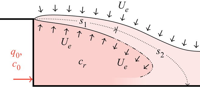
Figure 2. The neutral case. Exhaust flow per unit depth  $q_0$ is injected at the base of the step and well mixed into the recirculation region. Until point $s_1$ flow is entrained into the shear layer from the free stream and the recirculation region at rate $U_e$. Beyond $s_1$, until the point $s_2$, flow is entrained and detrained (as indicated) from the shear layer also at rate $U_e$. Points $s_1$ and $s_2$ are defined in § 2.1. The average value of pollutant concentration with the recirculation region is $c_r$. Diagram not to scale.
Additionally considering the fluxes of concentration into the shear layer and recirculation region allows for the time-average concentration within the shear layer ( $c_{sl}$) and the recirculation region ( $c_r$) to be found (Appendix B.2). The average concentration within the recirculation region is given by
 \begin{gather} c_r|_{Fr'\rightarrow \infty} = c_0 \frac{{\rm e}^{{1}/{2}} q_0}{U_es_1}, \end{gather}
 \begin{gather}\hat{c}_r|_{Fr'\rightarrow \infty} = \frac{c_r|_{Fr'\rightarrow \infty}}{c_0 \hat{q}_0} = \frac{{\rm e}^{{1}/{2}}}{\hat{U}_e\hat{s}_1}, \end{gather}
where  $\hat {s}_1 = s_1/H$. As outlined in figure 1(b), we wish to estimate the average concentration within an $H \times H$ region. If we assume the exhaust is quickly well mixed into the recirculation region and that the recirculation region fills the $H \times H$ zone, $\hat {c}$ can be modelled as being equal to $\hat {c}_r|_{Fr'\rightarrow \infty }$.
2.2 Modelling buoyant pollution dispersion
We now examine the effect of introducing buoyancy. When introduced, the buoyancy forces compete against the inertial forces in the wake. As buoyancy becomes more influential, it is expected that the inertial forces within the recirculation region will be overcome and a wall plume will form on the backward face of the step. When buoyancy is sufficiently strong, the entrainment into the plume will prevent a pollutant from being mixed directly into the recirculation region, but instead will rise up and into the shear layer. When it reaches the shear layer, the considerably higher inertial forces present there take over and the pollutant gets mixed into and follows the behaviour of the shear layer (figure 3a).

Figure 3. The effect of a buoyant pollutant. (a) When buoyancy is sufficiently strong, a dominant wall plume will form on the back of the step. The total entrainment flux per unit depth into the wall plume is  $q_{pe}$. Aspects of the model unchanged from the neutral exhaust model (2) are shown faded. The average values of concentration and buoyancy in the recirculation region are $c_r$, $g'_r$. (b) For slightly weaker buoyancy forcing, some of the pollutant will be mixed into the recirculation region as the plume rises. We denote the fraction of plume pollutant flux that reaches the shear layer as $\beta$. Diagrams not to scale.
As with the neutral exhaust, this scenario (figure 3a) can be modelled by considering volume and concentration fluxes into and out of the recirculation region, the shear layer and now additionally the plume. The entrainment flux per unit depth into the wall plume ( $q_{pe}$) can be derived from the plume entrainment assumption (see Reference TurnerTurner, 1973). As outlined in Appendix B.1, it is given by
 \begin{gather} q_{pe} = 3\alpha f_0^{1/3} H, \end{gather}
 \begin{gather}\hat{q}_{pe} = \frac{3\alpha}{Fr'}, \end{gather}
where  $\alpha$ is the entrainment coefficient for the plume ( $\alpha \approx 0.09$) and $3$ is a constant relating the characteristic plume velocity to the buoyancy flux (Reference Parker, Burridge, Partridge and LindenParker, Burridge, Partridge, & Linden, 2020).
There is a large range of intermediate behaviour where the exhaust buoyancy is not strong enough to overcome the inertial forces in the wake. In this range we model that a fraction  $0<\beta <1$ of the plume pollutant will make it directly into the shear layer as a result of its buoyancy whilst the remaining proportion ( $1-\beta$) is mixed into the recirculation region. Determining $\beta$ is key to modelling this intermediary behaviour. The value of $\beta$ will depend upon the ratio between a time scale for how quickly the buoyant pollutant can rise to the height of the shear layer ( $\tau _p$) and a time scale for how quickly the recirculation region can mix the pollutant ( $\tau _r$). Through dimensional considerations these two time scales can be determined as
 \begin{equation} \tau_p \equiv \frac{H}{f_0^{1/3}},\quad \tau_r \equiv \frac{H}{U},\quad \text{where}\ \frac{\tau_r}{\tau_p} = \frac{U}{f_0^{1/3}} = Fr', \end{equation}
where we note that  $f_0^{1/3}$ is a characteristic velocity scale of a line plume. This suggests that $\beta$ is a function of $Fr'$, and exhibits the behaviour that $\beta \to 1$ as $Fr' \to 0$ and $\beta \to 0$ as $Fr' \to \infty$. A function that fits this behaviour is an exponential:
 \begin{equation} \beta = \exp({-Fr'/Fr'_c}), \end{equation}
which is our modelling assumption for the functional dependence  $\beta (Fr')$. Here, $Fr'_c$ is a constant which can be thought of as a critical Froude number where the buoyancy forces match the inertial forces within the wake. This can be estimated by considering the flow speed within the wake, which from figure 5 can be seen to be approximately $0.03<|\boldsymbol {u}|/U<0.1$. This gives an estimate for the critical Froude number as $10< Fr'_c<30$.
Considering the concentration and volume fluxes into and out of the plume, the shear layer and the recirculation region (Appendix B), the normalised average pollutant concentration within the recirculation region can be found as a function of  $Fr'$ to be
 \begin{equation} \hat{c}_r = \frac{D(Fr') - \beta(Fr')}{\beta(Fr')\hat{q}_{pe} + \hat{U}_e\hat{s}_1}, \end{equation}
where  $\hat {q}_{pe}=q_{pe}/(UH)$ and $D$ is defined further below in (2.16a–d).
We wish to estimate the average concentration within an  $H \times H$ region immediately behind the step. As outlined in more detail in Appendix B.2, the fraction of the exhaust plume $\beta$ that is driven into the shear layer due to the buoyancy of the plume will also contribute to the total concentration during the period of time it takes the plume to rise to the shear layer. By assuming that the plume remains located within the $H\times H$ region, this contribution can be found to be $\beta Fr'/3$ when averaged over the $H\times H$ region. By assuming that the recirculation region fills the $H\times H$ zone, the prediction for $\hat {c}$ is then given by
 \begin{gather} \hat{c} = \frac{\bar{c}_{H\times H}}{c_0\hat{q}_0} = \frac{D - \beta}{\beta\hat{q}_{pe} + \hat{U}_e \hat{s}_1} + \frac{\beta}{3} Fr' , \end{gather}
 \begin{gather}D(Fr') = \exp\left(\frac{\beta \hat{q}_{pe} + \hat{U}_e\hat{s}_1}{\beta\hat{q}_{pe} + 2\hat{U}_e\hat{s}_1}\right), \quad \beta(Fr') = \exp({-Fr'/Fr'_c}), \quad \hat{q}_{pe}(Fr') = \frac{3\alpha}{Fr'}, \quad \hat{U}_e = \frac{E}{2}, \end{gather}
with  $\alpha$ being the entrainment coefficient for the plume and $E$ being the entrainment coefficient for the shear layer. The assumption that the recirculation region encompasses the $H\times H$ area is reasonable since the dip of the shear layer is very low for the majority of the shear layer as can be seen from PIV measurements in figure 5. As the shear layer develops, its width increases. This means that the shear layer slightly encroaches on the $H\times H$ region. However, the contribution of this encroachment is negligible and can be calculated to have an influence of less than $0.5\,\%$ upon the predicted value of $\hat {c}$.
As  $Fr' \rightarrow 0$ the value of $\hat {c}$ predicted by (2.15) approaches zero as $\hat {q}_{pe}\to \infty$ according to (2.16a–d) . At particularly low Froude numbers, the modelling assumptions will loose their validity: decreasing $Fr'$ by changing $U$ or $g_0'$ causes problems to arise with Reynolds invariance and the Boussinesq approximation, respectively. Increasing the exhaust flow rate per unit depth ( $q_0$) will break the assumption that $q_0$ is small and does not influence the flow structure.
3. Experimental methods
We now describe the experiments performed to test the model from the previous section. Experiments were performed within a recirculating water flume (figure 4a) with a working cross-section of  $300\,{\rm mm}\times 450\,{\rm mm}$ and flow speeds in the range of $73\unicode{x2013}133\,{\rm mm}\,{\rm s}^{-1}$. Two turbulence-damping meshes were placed upstream to improve the flow uniformity in the working section. The upstream contraction and the blockage ratio ( $10\,\%$) meet the criteria detailed by Reference Barlow, Pope and RaeBarlow, Pope, and Rae (1999) for maximum allowable blockage ratio within wind tunnels and water flumes. As shown in figure 4(b), the step is smoothly ramped up to its full height over a distance of $205.8\,{\rm mm}$ ( ${\sim }4.5H$) and then maintained at the full step height for $67\,{\rm mm}$ ( ${\sim }1.5H$). The step spans the entire width of the flume, which gives an aspect ratio of $AR = 6.7$. Reference Brederode and BradshawBrederode and Bradshaw (1973) and Reference Papadopoulos and OtugenPapadopoulos and Otugen (1995) investigated the influence of $AR$ upon the reattachment length, both finding that reattachment length increases with $AR$ until it levels off to a consistent value, occurring around $AR=5$, this also being a function of the expansion ratio of the step. With non-infinite aspect ratios, three-dimensional flow structures are still present, and Reference Hall, Behnia, Fletcher and MorrisonHall, Behnia, Fletcher, and Morrison (2003) find that the primary and secondary vortices spiral up to meet the top of the step at the sidewalls when observing a time-averaged flow structure. Reference Brederode and BradshawBrederode and Bradshaw (1973) considered an expansion ratio of $ER=1.11$, equal to that considered within this investigation, and found the reattachment length stabilised to $5.9$.

Figure 4. Experimental set-up. (a) The recirculating flume has a  $300\,{\rm mm}\times 450\,{\rm mm}$ cross-section and flow speeds of $73\unicode{x2013}133\,{\rm mm}\,{\rm s}^{-1}$. (b) The step smoothly ramps up to a height $H = 45\,{\rm mm}$ over a distance ${\sim }4.5H$ and remains at a constant height for ${\sim }1.5H$ giving an expansion ratio of $1.11$. Flow rates of $12.3 < q_0 < 27.9\,{\rm mm}^2\,{\rm s}^{-1}$ were used giving $0.015< U_0/U<0.064$, where $U_0$ is the speed of the exhaust flow and $U$ the free-stream flow speed. (c) Line source design. Exhaust passes through a brass plate with $1\,{\rm mm}$ diameter holes drilled at a spacing of $7\,{\rm mm}$. Flow then exits through a sharp-edged $6\,{\rm mm}$ gap at the base of the step.
The step is mounted on a Perspex floor which is  $600\,{\rm mm}$ long and the full width of the tank. A gear pump is used to pump a dyed saline solution through a line source at the base of the step (figure 4c). The tested values of $q_0$, the volume flux per unit depth, were $12.3,\ 17.4,\ 22.6 \text { and } 27.9\,{\rm mm}^2\,{\rm s}^{-1}$, which when combined with the range of flow speeds tested results in a range of $2.1<\hat {q}_0<8.5$ for the normalised exhaust flow rate per unit depth. The line source exhaust (figure 4c) was designed to trip the exhaust to turbulence, inspired by the Cooper plume nozzle (Reference Kaye and LindenKaye & Linden, 2004). The exhaust was passed initially through a brass plate with $1\,{\rm mm}$ diameter holes drilled at a spacing of $7\,{\rm mm}$.
The saline exhaust used in this investigation is negatively buoyant in comparison with the water used as the working fluid. The step and Perspex floor, as shown in figure 4(a), are inverted and as such are representative of a positively buoyant plume released behind an upward-facing step. We assume the flow is Boussinesq, i.e. that density differences are small and have negligible influence except where the difference is multiplied by acceleration due to gravity,  $g$. The experimental results are presented flipped, as many applications involve positively buoyant pollutants behind an upward-facing step.
Quantitative data were collected using PIV and dye attenuation measurements. The PIV technique was used to measure the velocity field behind the step in order to identify when the wake structure became Reynolds invariant. The PIV used  $55\,\mathrm {\mu }$m diameter neutrally buoyant polyamide particles and data were collected at 50 fps and analysed with PIVlab (Reference Thielicke and SonntagThielicke & Sonntag, 2021). A high-performance signal synchroniser was used to provide a stable DC power supply to the PIV light sheet. Flickering interference between the 50 fps frame rate and the 50 Hz mains AC power supply was not found to occur.
Back-lit dye attenuation, as outlined by Reference Allgayer and HuntAllgayer and Hunt (2012), is used to extract depth-integrated concentration profiles of the released ‘pollutant’. Dye attenuation data were collected at 20 fps. A methylene blue dye concentration of  $0.447\,{\rm mg}\,{\rm l}^{-1}$ was used. A description of the methods used, along with calibration curves and ranges of assumed linearity for the dye can be found in Appendix A.1. Further details of uncertainties in experimental measurements can be found in Appendix A.2.
As we are principally interested in applications at high Reynolds number, we performed a series of experiments to ensure our experiments were in the Reynolds-number-invariant regime. Reference Armaly, Durst, Pereira and SchönungArmaly et al. (1983) and Reference Nadge and GovardhanNadge and Govardhan (2014) both examined the backward-facing step at varying Reynolds numbers, finding that the reattachment length was Reynolds invariant around  $Re_{H} \sim 2\times 10^4$ for an expansion ratio of 1.1 (equal to the expansion ratio examined in this paper). Reference Tihon, Pěnkavovà, Havlica and ŠimčikTihon et al. (2012) also investigated the behaviour of reattachment length with Reynolds number, and found a sharp increase in reattachment length at low $Re_H$ which levels out around $Re_H = 800\unicode{x2013}1200$. Our experiments were performed at a higher $Re$ than that of Reference Tihon, Pěnkavovà, Havlica and ŠimčikTihon et al. (2012), but lower $Re$ than that of Reference Armaly, Durst, Pereira and SchönungArmaly et al. (1983) and Reference Nadge and GovardhanNadge and Govardhan (2014); therefore, we include PIV results demonstrating $Re_H$ invariance.
We varied the Reynolds number in the range  $370< Re_H<6000$, with PIV results for five selected Reynolds numbers shown in figure 5. There is a significant change to the general flow structure between $Re_H = 370$ and $Re_H = 880$ (figure 5a,b) with significantly fewer changes as $Re_H$ increases to $3300$, $4600$ and $5300$ (figure 5c–e). The reattachment length reached follows the pattern outlined by Reference Tihon, Pěnkavovà, Havlica and ŠimčikTihon et al. (2012) and our PIV experiments indicate that the overall structure of the wake behind the backward-facing step has reached Reynolds invariance at $Re_H \approx 3000$. This can further be seen by considering the change to the recirculation length with Reynolds number, see figure 5(f), in which the recirculation length reduces and plateaus at approximately $4.7H$. All subsequent experiments were performed above the determined critical Reynolds number, with experiments performed at $Re_H = 3300, 4600 \text { and } 6000$.

Figure 5. Reynolds number effects. (a–e) Time-averaged velocity profiles with streamlines for increasing Reynolds number  $Re_H = [370, 880, 3300, 4600, 5300]$. Free-stream flow speeds $U = [8,20,73,103,118]\,{\rm mm}\,{\rm s}^{-1}$. Dashed streamlines indicate $|\boldsymbol {u}|<0.1U$, where $\boldsymbol {u}$ is the local flow velocity. (f) Recirculation length ( $L_r$) plotted against Reynolds number. Invariance is observed for $Re_H\gtrsim 3000$.
4. Results
We now outline the experimental results. Figure 6(a,c,e) shows instantaneous false-colour concentration fields for three selected cases. Buoyancy has been introduced in the second, and increased further in the third. The profiles are produced using a dye attenuation technique (details in Appendix A.1), which results in depth averaging over the width of the flume. The shear layer confining the recirculation region can be observed with instabilities developing on the upper edge similar in appearance to classic Kelvin–Helmholtz instabilities, although they cannot be directly described as Kelvin–Helmholtz (except in the neutral exhaust case) due to the presence of an unstable density stratification in the direction of shear (see the supplementary information for videos available at https://doi.org/10.1017/flo.2023.14). As buoyancy is increased, less of the pollutant is trapped within the recirculation region, and instead is quickly transported up to the shear layer by the plume.

Figure 6. (a,c,e) Instantaneous concentration fields (using a natural logarithmic scale) and (b,d,f) time-averagedconcentration fields (using a logarithmic scale) with PIV streamlines overlaid, for varying adapted Froude number  $Fr' = U/(q_0 g'_0)^{1/3}$: (a,b) $\infty$; (c,d) $9.9$; (e,f) $6.4$. The flow speed was $U = 73\,{\rm mm}\,{\rm s}^{-1}$ ( $Re_H =3300$) and the exhaust flow rate (per unit depth) $q_0 = 27.9\,{\rm mm}^2\,{\rm s}^{-1}$. The buoyancy of the pollutant was varied as $g'_0 = [0, 14.3, 51.7]\,{\rm mm}\,{\rm s}^{-2}$.
Figure 6(b,d,f) shows time-averaged concentration fields for the three cases considered. The profiles were time-averaged over 90 s. The convergence of these profiles was checked by increasing the averaging time until the mean concentration within an  $H\times H$ region behind the step had stabilised. This was found to converge after ${\sim }45\,{\rm s}$. Streamlines, derived from PIV from experiments performed at similar Froude numbers ( $Fr' = [\infty,\ 10.9,\ 7.1]$), have been overlaid on the concentration fields. The macrostructure of the wake is unchanged through the addition of buoyancy. Small changes between the three profiles can be noted close to and towards the base of the step. It should be noted that this coincides with the region where the PIV is less accurate due to the combination of significantly slower flow speeds and refractive index issues relating to the salinity of the exhaust.
From figure 6(b), it can be seen that at high  $Fr'$ the pollutant becomes close to well mixed within an $H\times 1.5H$ rectangle behind the wake, with pollutant transport dominated by the inertial forces of the recirculation region. The pollutant is eventually pushed up into the shear layer by the strong primary vortex. As the $Fr'$ number decreases, the strength of the buoyancy begins to overcome the inertial forces in the wake and buoyancy transports the pollutant directly into the shear layer rather than being mixed into the recirculation region (figure 6d). As the $Fr'$ number is decreased further, the buoyant pollutant sticks more closely to the wall of the step, forming a structure analogous to a wall plume (figure 6f). At intermediary stages, the buoyant plume attaches and detaches due to unsteady fluctuations in the inertial forces in the wake. This behaviour will also be dependent upon the exhaust momentum, an effect we have neglected in this investigation. The velocity scales within the recirculation region are significantly lower than those in the free stream and the shear layer (see figure 5); therefore as the influence of buoyancy is increased it first overcomes the inertial forces within the recirculation region. We expect that as buoyancy is increased further, it will begin to influence the shear layer and macrostructure of the wake; however, this was not clearly observed experimentally within the range of $Fr'$ that we were able to achieve while keeping the experiment in the Reynolds ( $Re_H$)-invariant regime. The neutral exhaust flow in figure 6(b) might appear to show a strong exhaust jet which clings to the floor up until approximately $H$, which would contradict the previous assumption that the exhaust momentum is negligible. However, the strength of this exhaust jet is exaggerated by the secondary recirculation vortex which pushes pollutant in the direction of the exhaust jet. As buoyancy is increased in figure 6(d,f) and buoyancy begins to overcome the inertial forces in the secondary vortex, the jet width reduces to $0.25H$.
The effect of  $Fr'$ can be seen further in figure 7, which shows vertical profiles of time-averaged concentration at three distances from the step with increasing $Fr'$. These profiles can be thought of as vertical lines taken from figure 6(b,d,f). The highest buoyancy case (lowest $Fr'$, yellow) has a reduced concentration trapped immediately behind the step compared with the lowest and neutral buoyancy (high $Fr'$, purple). This reduction is consistent from $x/H=1$ to $x/H=3$ (figure 7a,c), although further from the step the relative reduction in concentration is smaller. Furthermore, there is a noticeable shift upwards in the location of the peak concentration behind the step as buoyancy increases. Initially, because the pollutant is being advected and dispersed by the recirculation region, a fairly flat distribution is observed with the neutral case showing a peak concentration very low to the ground. As the influence of buoyancy increases ( $Fr'$ decreases) the wall plume develops and pushes the pollutant into the shear layer, shown through the presence of a distinct peak occurring around $z/H \sim 0.8$ at $x/H = 1$. At still lower $Fr'$ it is expected that this peak would move upwards as the strength of the buoyancy within the shear layer begins to overcome the inertial forces of the shear layer.

Figure 7. Vertical profiles of concentration at varying distances downstream of the step: (a)  $x/H=1$, (b) $x/H = 2$ and (c) $x/H = 3$. All $x$ axes have equal proportioned scales. The flow rate was $U = 73\,{\rm mm}\,{\rm s}^{-1}$ and the exhaust flow rate per unit depth was $q_0 = 22.6\,{\rm mm}^2\,{\rm s}^{-1}$. The Froude number was varied by changing the buoyancy as $g'_0 = [0,\ 5.54,\ 8.45,\ 14.3,\ 31.9,\ 51.7]\,{\rm mm}\,{\rm s}^{-2}$.
The reduction in pollutant trapped behind the step can be quantitatively examined by averaging the concentration in an  $H \times H$ square behind the step ( $\bar {c}|_{H \times H}$). Figure 8 shows $\hat {c}$ plotted against the adapted Froude number $Fr'$, where $\hat {c}$ is $\bar {c}|_{H \times H}$ divided by $c_{0}\hat {q}_0$ as defined in (2.1a–c). The data points in figure 8 represent a systematic variation of the exhaust buoyancy ( $g'_{0} = [0,\ 5.54,\ 8.45,\ 14.3,\ 31.9,\ 51.7]\,{\rm mm}\,{\rm s}^{-2}$), the exhaust flow rate ( $q_0 = [12.3,\ 17.4,\ 22.6,\ 27.9]\,{\rm mm}^2\,{\rm s}^{-1}$) and the free-stream flow speed ( $U= [73,\ 103,\ 133]\,{\rm mm}\,{\rm s}^{-1}$).
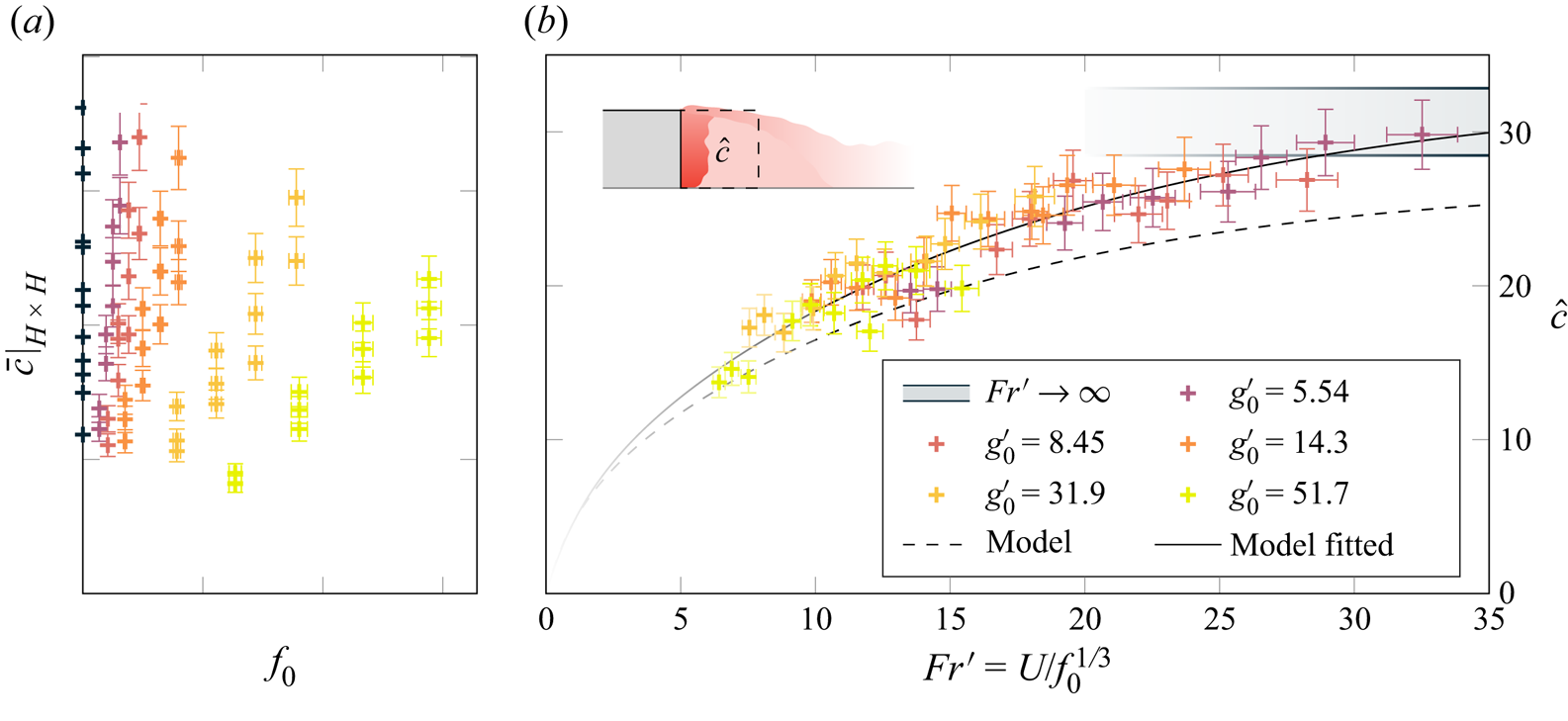
Figure 8. The effect of buoyancy on the concentration of pollutant trapped behind a step. (a) Average concentration within an  $H\times H$ region behind the step plotted against exhaust buoyancy flux. (b) Average non-dimensional concentration $\hat {c}$ behind the step versus the adapted Froude number $Fr'$. The flow speed was varied as $U = [73\ 103\ 133]\,{\rm mm}\,{\rm s}^{-1}$ along with the exhaust flow rate per unit depth as $q_0 = [12.3\ 17.4\ 22.6\ 27.9]\,{\rm mm}^2\,{\rm s}^{-1}$ and the exhaust buoyancy as $g'_0 = [\text {see legend}]\,{\rm mm}\,{\rm s}^{-2}$. Dashed line represents model (2.15) with expected model parameter values and solid line shows the model with fitted parameter values (see table 1).
Figure 8(a) shows the average concentration behind the step against the buoyancy flux. Figure 8(b) shows how these data collapse onto a curve displaying the asymptotic behaviour predicted by the theory developed in § 2. The dashed line shows the model from (2.15) and (2.16a–d) with the parameters  $E$,
$E$,  $\alpha$ and $Fr'_c$ fitted with a least-squares method to the data. A comparison between the predicted values and the fitted values can be found within table 1. Parameter $\hat {s}_1$ is taken as half the length of the shear layer, which is taken to be half of the length of the recirculation region.
Table 1. Model parameters. Comparison of predicted with fitted values. Fit performed with a least-squares method, and values shown to two significant figures.
 $^{a}$Derived from Reference RajaratnamRajaratnam (1976). $^{b}$Reference TurnerTurner (1973) and Reference Parker, Burridge, Partridge and LindenParker et al. (2020). $^{c}$Expected range from order-of-magnitude considerations in § 2.2.
The exhaust flow rate was assumed to be small ( $\hat {q}_0 \ll 1$). To check the validity of this assumption, we can substitute the range of values for $\hat {q}_0$ used into the model. We find this changes the estimate for $\hat {c}$ by a maximum of 4 %.
5. Conclusions and discussion
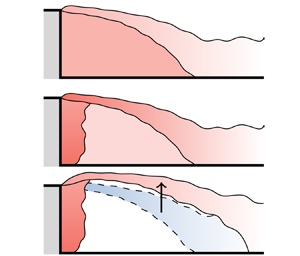
We have investigated the effect of buoyancy on pollutant dispersion behind a backward-facing step. We have identified the transition between two main regimes, depending on the relative strength of the buoyancy of the pollutant and the inertia of the surrounding flow, as measured by an adapted Froude number,  $Fr'$. When the effect of buoyancy is weak ( $Fr'\gtrapprox 25$) pollutant dispersion is driven entirely by advection in the wake (figure 9a). As the buoyancy of the pollutant is increased (moderate $Fr' \lessapprox 15$), buoyancy-driven convection dominates relative to inertial forces within the recirculation region but remains negligible in comparison with the inertial strength of the shear layer (figure 9b). As a result, in this regime the pollutant trapped behind the step reduces, but the shape of the wake is unaffected. A third regime is hypothesised to exist below the range of $Fr'$ tested in our study ( $7< Fr' < \infty$) where buoyancy becomes sufficiently strong to influence the height of the shear layer and the overall shape of the wake (figure 9c).

Figure 9. Three regimes. (a) High  $Fr'$: pollutant is advected and dispersed by the recirculation region. (b) Moderate $Fr'$: a wall plume develops and feeds directly into shear layer. The concentration of pollutant trapped behind the step decreases. (c) Low $Fr'$: increasing buoyancy starts to influence the shape of the wake and location of the shear layer.
A theoretical steady-state model was developed to determine the average pollutant concentration held within the recirculation region and how it changes with  $Fr'$. The model predicts the pollutant trapped in this region to decrease as the influence of buoyancy is increased (decreasing $Fr'$). The experimental results were found to compare well with the model predictions, with three fitted parameters. The values of these fitted parameters were close to estimates derived from further modelling.
This paper has begun to quantify how buoyancy changes the dispersion and transport of a pollutant whilst also subject to the inertial forces in the wake of a backward-facing step. This work can feed into future research into the effect of buoyancy on car exhaust dispersion, along with other important urban pollution transport problems, such as the dispersal of pollution behind buildings.
Appendix A. Experimental methods
A.1 Dye calibration
The dye (methylene blue) used to extract approximate pollutant concentrations through dye attenuation does not perfectly follow the assumed Lambert–Beer attenuation law:
 \begin{equation} \ln \left(\frac{I}{I_0}\right) \propto{-}hc, \end{equation}
where  $I$ is the light intensity recorded by the camera, $I_0$ is the background light intensity (Reference Allgayer and HuntAllgayer & Hunt, 2012), $h$ is the depth of the attenuating specimen and $c$ is the dye concentration. Nonlinearity is introduced due to a range of wavelengths of light being used during the experiment, an appropriate red filter being used to minimise this. The actual attenuation and the assumed range of linearity are shown in figure 10.

Figure 10. Methylene blue calibration curve and histogram of pixel values within an instantaneous shot of the  $H\times H$ region behind the step with a neutral exhaust being expelled. Here $c_0$ has a methylene blue concentration $0.447\,{\rm mg}\,{\rm l}^{-1}$, with this calibration curve being specific to the lighting, camera and camera settings of this investigation.
Figure 10 also displays a histogram showing the distribution of pixel values of  $\ln (I/I_0)$ within an $H\times H$ square behind the step for an instantaneous snapshot of a neutral exhaust experiment. It can be found that $97.9\,\%$ of pixel values fall within the assumed range of linearity. The total error for the estimated average concentration within an $H \times H$ square ( $\hat {c}$) can be calculated from the two plots in figure 10 and found to be 4.9 % due to nonlinearity in dye attenuation.
A.2 Error analysis
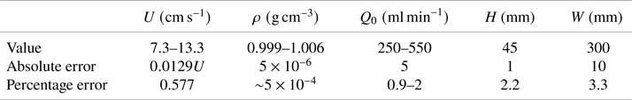
Table 2 lists the parameters considered within this investigation, the range of values considered and absolute errors associated with each value. From this the percentage errors for each quantity can be found and combined to find the errors associated with the final presented quantities.
Table 2. Errors associated with fundamental measured quantities.
Appendix B Modelling the wake
B.1 Modelling the plume
The plume is modelled as if it is acting in an ambient and still environment.
Entrainment velocity into the plume is proportional to the characteristic plume velocity, related by the entrainment constant  $\alpha$ (Reference TurnerTurner, 1973). The velocity within a wall plume is assumed to be self-similar and proportional to the cube root of exhaust buoyancy flux $f_0^{1/3}$ with a proportionality factor of $3$ (Reference Parker, Burridge, Partridge and LindenParker et al., 2020; Reference TurnerTurner, 1973). Integrating this for $0< z< H$ gives the total plume entrainment flux per unit depth as
 \begin{gather} q_{pe} = 3 \alpha f_0^{1/3} H, \end{gather}
 \begin{gather}\hat{q}_{pe} = \frac{q_{pe}}{UH} = \frac{3\alpha}{Fr'}, \end{gather}
where  $\hat {q}_{pe}$ is the normalised plume entrainment flux. Evaluating the volume and concentration fluxes into the plume, the volumetric flux ( $q_p$) and average concentration ( $c_p$) at the top of the plume after entrainment can be found to be
 \begin{gather} q_{p} = q_{pe} + q_0 \approx q_{pe}, \end{gather}
 \begin{gather}c_{p} = \frac{q_{pe}c_r + q_0 c_0}{q_p}. \end{gather}
In § 2.2, we outline that we expect a certain proportion of the plume ( $\beta q_p$) to rise directly into the shear layer as a result of the plume buoyancy with the remaining fraction ( $[1-\beta ] q_p$) being mixed back into the recirculation region (see figure 3b).
When estimating the average concentration  $\bar {c}_{H\times H}$ within the $H\times H$ region (2.15), the contribution of the pollutant that is held within the plume that will not be well mixed into the recirculation region needs to be considered. At each time point, the plume transports directly into the shear layer a fraction $\beta c_0 q_0$ of the exhaust pollutant flux (the contribution $\beta c_r q_{pe}$ is accounted for in Appendix B.2). The total additional pollutant amount due to the plume ( $C_p$) can be estimated using the exhaust flow rate multiplied by the time scale associated with how long it takes the plume to reach the top of the step. This gives
 \begin{gather} C_p = \beta c_oq_0 \frac{H}{3f_0^{1/3}}, \end{gather}
 \begin{gather}\hat{C}_p = \beta \frac{U}{f_0^{1/3}} \frac{H^2}{3} = \beta\frac{Fr'H^2}{3}, \end{gather}
where  $3f_0^{1/3}$ is the characteristic velocity associated with a wall plume (Reference Parker, Burridge, Partridge and LindenParker et al., 2020) and $\beta = \beta (Fr')$ accounts for the proportion of the plume that is expected to reach the shear layer without being mixed into the recirculation region (see (2.13)). Equation (2.15) considers the average pollutant concentration within the $H\times H$ region. Assuming that the plume remains within this region, the average contribution due to the plume can be found to be
 \begin{equation} \hat{c}_p = \beta \frac{Fr'}{3}.\end{equation}
B.2 Modelling the shear layer and recirculation region
In this section, we consider the fluxes into and out of the shear layer in order to determine the concentration profile within the shear layer. This will allow the average concentration  $c_r$ within the recirculation region to be calculated. We consider the general case where a fraction $\beta$ (2.13) of the exhaust plume rises directly into the shear layer due to the buoyancy of the exhaust, with the remaining fraction $1-\beta$ being well mixed into the recirculation region. To consider the neutral case, we set $\beta =0$. We make the assumption that the exhaust volumetric flux is small in comparison with other volume fluxes, except where it contributes to the exhaust concentration flux, such that
 $$\begin{gather} q_0 \ll q_{ * },\quad q_0 c_0 \sim q_{{ * }}c_{ * }, \end{gather}$$
where  $q_{*}$ and $c_{*}$ represent generic volume fluxes and concentrations considered within this investigation. The following modelling could be performed without the assumption that $q_0$ is small; however, the modelling assumption that the exhaust does not alter the flow structure would no longer be valid and further complex modelling would be required.
Figure 11(a) shows a control volume outlining the fluxes into and out of the shear layer up until the flow reversal point  $s_1$. Balancing these fluxes, we can find the average flow rate and average concentration within the shear layer at $s_1$ to be
 \begin{gather} q_{sl}(s_1) = \beta q_{pe} + 2U_es_1, \end{gather}
 \begin{gather}c_{sl}(s_1) = \frac{\beta c_0q_0 + c_r(\beta q_{pe} + U_es_1)}{\beta q_{pe} + 2U_es_1}. \end{gather}
After point  $s_1$, the flow is detrained out of the shear layer and back into the recirculation region. We assume here that the detrainment velocity $U_d$ out of the shear layer into the recirculation region has the same magnitude as the entrainment velocity, namely $U_d=U_e$. Figure 11(b) shows the fluxes into and out of a small control volume of length $ds$ after the point of entrainment reversal $s_1$. By considering this small control volume and a new streamwise coordinate ( $s'=s+s_1$), we can derive the average shear layer concentration $c_{sl}$ after the flow reversal as a function of $s'$:
$s'$:
 \begin{equation} c_{sl}(s') = c_{sl}(s_1)\exp\left(-\frac{U_e s'}{q_{sl}(s_1)}\right). \end{equation}
Integrating the detrainment velocity multiplied by  $c_{sl}(s')$ over the length $s_2$ gives the total concentration flux from the shear layer into the recirculation region:
 \begin{align} \int^{s_2}_0 c_{sl} U_e \,{\rm d} s' & = c_{sl}(s_1)q_{sl}(s_1) \left[ 1-\exp\left(-\frac{U_e s_2}{q_{sl}(s_1)}\right) \right] \end{align}
 \begin{align} & = [\beta c_0 q_0 + c_r(\beta q_{pe} + U_e s_1)] \left[ 1-\exp\left(-\frac{U_e s_2}{q_{sl}(s_1)}\right) \right]. \end{align}
Balancing the concentration fluxes into and out of the recirculation region,
 \begin{equation}
\underbrace{c_rq_{pe}}_{Entrainment\ into\ plume} +
\underbrace{c_rU_es_1}_{Entrainment\ into\ shear\ layer}
= \underbrace{\int^{s_2}_0 c_{sl} U_e \,{\rm d}
s'}_{Detrainment} + \underbrace{(1-\beta)(q_{pe}c_r
+ coq_0)}_{Fraction\ of\ plume\ mixed\ into\ RR},
\end{equation}
\begin{equation}
\underbrace{c_rq_{pe}}_{Entrainment\ into\ plume} +
\underbrace{c_rU_es_1}_{Entrainment\ into\ shear\ layer}
= \underbrace{\int^{s_2}_0 c_{sl} U_e \,{\rm d}
s'}_{Detrainment} + \underbrace{(1-\beta)(q_{pe}c_r
+ coq_0)}_{Fraction\ of\ plume\ mixed\ into\ RR},
\end{equation}
see figure 11(c), an expression for the normalised average concentration within the recirculation region  $\hat {c}_r$ can be found as
 \begin{equation} \hat{c}_r = \frac{c_r}{c_0\hat{q_0}} = \frac{D - \beta}{\beta\hat{q}_{pe} + \hat{U}_e \hat{s}_1}, \end{equation}
where
 \begin{equation} D = \exp\left(\frac{\hat{U}_e \hat{s}_2}{\hat{q}_{sl}(s_1)}\right) = \exp\left(\frac{\hat{U}_e \hat{s}_2}{\beta \hat{q}_{pe} + 2\hat{U}_e\hat{s}_1}\right). \end{equation}
By considering conservation of volume within the recirculation region, we can relate the length  $\hat {s}_2$ to $\hat {s}_1$ as
 \begin{equation} \hat{U}_e\hat{s}_2 = \hat{U}_e\hat{s}_1 + \beta \hat{q}_{pe}, \end{equation}
therefore simplifying the expression for  $D$ to
 \begin{equation} D = \exp\left( \frac{\beta \hat{q}_{pe} + \hat{U}_e\hat{s}_1}{\beta\hat{q}_{pe} + 2\hat{U}_e\hat{s}_1} \right). \end{equation}
Note that for the case of the neutral exhaust  $\beta =0$, we recover $\hat {s}_1=\hat {s}_2$.

Figure 11. Simplified shear layer control volumes, where  $q_{sl}$ is the shear layer volume flux, $c_{sl}$ is the average shear layer concentration, $U_e$ is the entrainment velocity, $c_r$ is the average recirculation region concentration and $c_0$ and $q_0$ are the exhaust concentration and flow rate per unit depth. (a) Control volume before entrainment reversal, valid over length $s_1$. (b) Small control volume after entrainment reversal, valid over length $s_2$. (c) Wake control volumes. This figure is a collation of figures 2, 3(a) and 3(b). Not to scale.
As outlined in § 2 and figure 1(b), we wish to estimate the average concentration  $\bar {c}_{H\times H}$ within an $H \times H$ region immediately behind the step. The fraction of the exhaust concentration flux $\beta c_0 q_0$ that is driven directly into the shear layer due to the buoyancy of the plume also contributes to the total concentration $\bar {c}_{H\times H}$ during the period of time it takes for the plume to rise to the shear layer; see (B.5). It should be noted that the plume also contains the contribution $(1-\beta ) c_0 q_0$. However, this contribution is already taken into consideration when calculating $c_r$, see (B14), allowing an estimate for the total concentration:
 \begin{align} \hat{c} & = \frac{\bar c_{H\times H}}{c_0\hat q_0} \end{align}
 \begin{align} & = \hat{c}_r + \hat c_p \end{align}
 \begin{align} & = \frac{D - \beta}{\beta\hat{q}_{pe} + \hat{U}_e \hat{s}_1} + \frac{\beta}{3} Fr', \end{align}
where we used (B.7) and (B15). Here, if we consider the neutral exhaust ( $Fr'\rightarrow \infty$ and $\beta =0$) the following value of $c_r$ is produced:
 \begin{equation} \hat{c}|_{Fr'\rightarrow \infty} = \frac{{\rm e}^{{1}/{2}}}{\hat{U}_e\hat{s}_1}. \end{equation}
As  $Fr' \rightarrow 0$, the value of $\hat {c}$ predicted by (B21) approaches zero ( $\hat q_{pe}\to \infty$; see (B.2)). As outlined within the main body of the text (§ 2.2), it is expected that the model assumptions do not describe the behaviour at very low $Fr'$ due to the exceptionally high exhaust buoyancy needed to produce low values of $Fr'$.
An assumption of this model is that the detrainment velocity  $U_d$ along the streamwise distance $s_2$ from the shear layer back into the recirculation region is equal to the entrainment velocity ${U}_e$ along $s_1$, i.e. $U_d=U_e$, and both do not vary with $s$. For the neutrally buoyant case, this implies $s_1 = s_2$.
We now briefly consider what happens if the assumption  $U_d=U_e=\textrm {const.}$ is dropped. There are two main mechanisms which could invalidate this assumption.
First, we consider the case where the entrainment velocity scale changes as the shear layer develops, i.e. the assumption of invariance with  $s$ is dropped. This might be expected since the flow that is drawn back into the recirculation region will provide a non-zero lower velocity boundary condition along $s_2$. We thus consider that along $s_2$, there is a simultaneous increase in the magnitude of entrainment velocity $U_{e,s_2}>U_e$ and the detrainment velocity $U_d=U_{e,s_2}$. By considering the volume conservation in the recirculation region in (B17) with $U_d s_2$ and the resulting substitution into (B8a,b), it can be found that the value of $D$ and therefore $\hat {c}$ is not influenced.
Second, we consider the case where the detrainment velocity  $U_d$ is not equal to the entrainment velocity $U_e$, i.e. $U_d\neq U_s$, over the length $s_2$. By investigating the behaviour of the shear layer we find that $\hat {c}_r$ can be found to be dependent on $U_d$ and by consequence $s_2$. A brief numerical estimate (not included here) shows that a 10 % increase in $\hat {s}_2$ produces a 6 % change in $\hat {c}_r$. However, from PIV results (see figure 5), we can see that we do not expect a large variation of $\hat {s}_2$, with $\hat {s}_2$ being close to the value of $\hat {s}_1$. Additionally, given the first-order nature of this model, it was felt that this offers an acceptable level of uncertainty for the expected uncertainty in $\hat {s}_2$.
Acknowledgements
The authors would like to thank J. Olsthoorn for reviewing a draft of this paper and the members of staff of the Engineering Department for the help with experimental set-up and maintenance.
Supplementary movies
Supplementary movies are available at https://doi.org/10.1017/flo.2023.14. Raw data are available from the corresponding author (S.C.).
Funding statement
The authors gratefully acknowledge funding by the EPSRC under grant numbers EP/N509620/1 and EP/R513180/1.
Declaration of interests
The authors declare no conflict of interest.
Author contributions
S.C. and M.D.W. created the research plan, designed experiments and formulated the analytical problem. S.C. led model development, performed the experiments and wrote the manuscript with M.D.W. providing providing edits, comments and feedback.


 Open access