


Introduction
Although near-surface processes leading to the formation of typical weak layers (e.g. surface hoar and near-surface faceted crystals) are fairly well understood, much less is known about the evolution of these weak layers once they are buried. Field and laboratory measurements of the evolution of snow properties, including detailed characterization of the grain shape and texture, are needed to improve model simulations of the evolution of snowpacks. Such models are needed to help professional avalanche forecasters identify potential weak layers in snowpacks.
The purpose of this study was to follow one such layer during its formation, as well as over a longer period of time once buried. An attempt was made to relate the field observations and measurements as well as a preliminary analysis of the grain shapes done in the laboratory to the output of numerical simulations.
Experimental Work
Development and Description of the Weak Layer
January 1996 was markedly poor in snowfalls at the study site of the Swiss Federal Institute for Snow and Avalanche Research on Weissfluhjoch/Davos, 2540 ma.s.1. By 11 January, less than 11cm of low-density snow (70–110kgm-3) had accumulated over an approximately 90 cm deep snow cover, the mean density of which was 260 kg m-3 (see Fig. 1). The meteorological conditions of the following days favoured the formation of a 5 mm thick surface crust. By 15 January, metamorphism of the fragmented precipitation crystals just below the crust had already resulted in the formation of faceted grains (see Table 1). Due to continuing clear weather, the layer below the crust was 1.5 2 cm thick by 24 January and consisted of faceted grains. This layer not only distinguish itself from the underlying layer by its grain shape, grain-size and density but also by a distinctive columnar-like texture (sec Fig. 2b and c). By the end of January, more and more cup-shaped crystals arranged in columns could be observed in this layer (see Fig. 3b and c; Table 1).
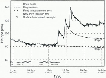
Fig. 1. Snow depth (automatic measurement) and height of temperature sensors within the snow cover at the study site on Weiss-fluhjoch. Solid line is measured snow depth. Doited and broken lines are the heights of harp and fixed temperature sensors, respectively (see text). Crosses and the numbers beneath indicate new snow (in cm) and “V” represents surface-hoar formation overnight, both recorded around 0700 h UTC.
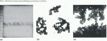
Fig. 2. (a) 1 cm thick translucent profile of the weak layer taken from the field on 12 February 1996. The dotted line shows the position of the top of the crust, (b) Broken weak layer and (c) isolated grains and grain clusters after preparation in the cold laboratory. The size of both pictures is approximately 17 x 17 mm2.
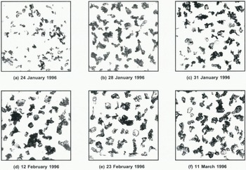
Fig. 3. Grains from the weak layer taken on six different days in the field and subsequently pictured in the cold laboratory. The size of all six pictures is 25 x 25 mm2.
Table 1. Comparison of grain characterizations. For the layers, u = upper, w= weak, l = lower. The apparent diameter was inferred from the surface of the grains obtained by digitizing pictures taken in the laboratory (Reference MarboutyMarbouty, 1980). The length of columns determined from pictures taken in the laboratory refers to a chain or column of cup-shaped crystals. Dendricity and sphericity have been described by Reference Brun, David., Sudul and BrunotBrun and others (1992)

More new snow (less than 5 cm, ρ = 70–110 kgm-3) accumulated over a period of 4 days around 26 January. Following the storm, clear weather conditions prevailed until 2 February. The layer was finally buried by snowfalls around 8 February and persisted in the snow cover until at least mid-April.
After being buried, the layer described above revealed itself to be a typical weak layer. Indeed, shear-frame measurements done 1 week after burial at the study site yielded a very low shear strength of 323 ± 134 Pa (0.05 m2 shear frame, corrected for size effects), as compared to a median value of (1000 ± 500) Pa for this type of snow (depth-hoar and/or surface-hoar) (Reference Föhn, Camponovo and Krusi.Föhn and others, 1998) Furthermore, because high-pressure conditions were prevailing over a large part of the eastern Swiss Alps, layers with very similar structures were found in various locations; several fatal skier-triggered slab avalanches resulted from them.
The formation of depth hoar and/or faceted crystals near the surface has gained renewed attention recently (Reference ColbeckColbeck, 1989; Reference Fukuzawa and Akitaya.Fukuzawa and Akitaya, 1993; Reference Birkeland, Johnson and SchmidtBirkeland and others, 1997), especially because it is prone to form weak layers once buried. The basics of depth-hoar formation, as described for example by Reference AkitayaAkitaya (1974), Reference MarboutyMarbouty (1980) and Reference ColbeckColbeck (1983), are also valid near the surface. However, the very strong gradients in excess of 100°Cm -1 recorded just below the surface may lead to rapid kinetic growth of crystals in lower-density snow (Reference Fukuzawa and Akitaya.Fukuzawa and Akitaya, 1993). Although we cannot reconstruct the formation of our weak layer in detail, we assume that rapid kinetic growth due to high gradients (> 50°Cm-1) took place during its formation period.
Field Work
In addition to weekly stratigraphic snow profiles at the study site, we followed the evolution of the weak layer more closely: from 25 to 31 January, daily in the morning before the study site was affected by the Sun, and after burial by new snow twice a week until 11 March. Temperature profiles from the lop of the snow cover to at least 10 cm below the weak layer were recorded at a spacing of 2 5 cm. The weak layer and adjacent layers were characterized and sampled in sub-freezing iso-octane for subsequent detailed analysis of the texture in the cold laboratory (Fig. 3) (Reference Brun and Pahaut.Brun and Pahaut, 1991). Furthermore, on 12 February and 11 March, 20 x 20 x 30cm3 blocks containing the weak layer were taken to the cold laboratory to prepare samples for detailed structural analysis and to make translucent profiles of the weak layer and its adjacent layers (sec Fig. 2).
Automatic Measurements
Our study site is well equipped to measure relevant meteorological parameters automatically. Air temperature, relative humidity, wind speed and wind direction, both incoming and outgoing short- and longwave radiation, precipitation and snow depth are available on a 1/2 hour basis.
Two arrays of sensors were used to record the temperature profile within the snow cover with an overall accuracy of ± 0.5°C. The first used thermistor sensors with a fixed vertical spacing of 20 cm, protruding about 20 cm horizontally from a central pole into the snow cover and arranged star-like (120° from sensor to sensor) in order to minimize the disturbance on settling of the snow cover. The second type of sensor was shaped like a harp: 7.5 m of tungsten wire (0.05 mm diameter) tightened on a 30 x 30 cm2 balsa-wood frame. Two sides of the frame are 11 cm longer, ending with spring-like contacts. Prior to a snowfall, these sensors are laid flat on the snow surface and the spring com acts are connected to two vertically fixed wires, which act both as a guide to the harp and as a potentiomctric measure of the harp’s depth, i.e. of the settling. The temperature-dependent resistivity of the tungsten wire allows us to measure snow temperature. Due to a careful calibration of infrared thermometers done at SFISAR (personal communication from P. Weilenmann, 1997), the snow-surface temperature could also be accurately measured to within ± 0.5°C.
At the site of the fixed temperature sensors, the January snow depth ranged from 95 cm at the beginning, to 85 cm around mid-January and to about 82 cm at the end of the month. During this time, the fixed sensor closest to the surface was 80 cm above ground. Thus, a fairly good estimate of the temperature gradients near the surface could be obtained at night-time over the formation period of our weak layer, i.e. in the second half of January. This will be discussed further below.
On 26 January, a harp was put on the surface of the snow cover. Fully buried by the snowfalls of 8 and 9 Febru-ary, this harp recorded the temperature at the depth of the weak layer. Another harp laid out on 14 February settled rapidly with the new snow. After 19 February, the vertical distance between the two harps was less than 20 cm and finally 14.4 cm on 11 March.
Model Simulations and Results
Description of Simulation Runs
Two physically based models for the simulation of the snow cover were used. The first model, called Crocus, was developed at the Centre d’Etudes de la Neige in Grenoble by Reference Brun, Martin, Simon, Gendre and Coleou.Brun and others (1989). It requires air temperature, wind speed, relative humidity, liquid precipitation, incoming longwave radiation, direct and diffuse shortwave radiation and cloudiness as inputs. In addition to temperature distribution, settling, phase changes and meltwater run-off, the model simulates the metamorphism of the deposited snow layers (Reference Brun, David., Sudul and BrunotBrun and others, 1992). New snow depth is estimated from liquid precipitation, air temperature and wind speed. Accordingly, total snow depth may differ from that measured in situ and therefore leads to some difficulties when comparing model outputs with field measurements. However, the date of the snowfall is recorded, thus allowing study of the layer’s evolution to follow. Two runs were initiated: the first from 10 January 1996, taking our weekly stratigraphic profile as an initial profile for the model, the second from 1 November 1995 with no snow on the ground. Both runs ended in the middle of june 1996. As the output of both runs did not differ by much, we shall use only the results of the second run for further comparisons with the observed evolution of our weak layer. The second model was a simplified version of the model Daisy developed at SFISAR by Reference Bader and Weilenmann.Bader and Weilenmann (1992). Using incoming shortwave radiation, surface temperature and the measured snow depth as input, the model simulates the temperature distribution and settling of the snow cover, taking into account phase changes. The model was initialized on 6 January with a measured temperature and density profile. As snow depth and surface temperature are input parameters, the half-hourly model outputs can be conveniently compared to measured temperature profiles.
Temperature Gradients and Temperature of the Snow Cover
For the 161+58 formation period of the weak layer (11 January– 5 February), Figure 4a shows the mean temperature gradient between 80 and 60 cm height, both measured with the fixed sensors and calculated by Daisy. Also shown are values calculated by Crocus for corresponding levels from the surface (differing snow depths!). The z axis is taken as positive from the ground. First, we note that the gradient is usually stronger than –20°Cm-1, especially at night. Secondly, the time-dependence of both measurements and calculations agree quite well over the whole period. However, there is a systematic positive bias of the measurements with respect to the simulated values. The same applies to the temperature a few centimetres below the surface (see Fig. 4b). During daytime, the strong influence of incoming shortwave radiation on the topmost fixed sensor at 80 cm leads to an overestimation of the temperature, whereas at night two effects may add up. First, the topmost sensor docs not cool down properly, as it is slightly covered by snow and, secondly, the model underestimates the heat conduction, e.g. because of calculated densities that are too low. Therefore, the temperature recorded by the topmost fixed sensor is always positively biased and leads to the observed discrepancy.
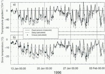
Fig. 4. Near-surface temperature gradient and temperature from 11 January until 5 February 1996. (a) Temperature gradient: solid line is evaluated from fixed sensors at 80 and 60 cm height. Broken line is the mean gradient between 80 and 60 cm as calculated by Daisy. ![]() is the mean gradient calculated by Crocus for corresponding levels from the surface (differing snow depths!). (b) Temperature: solid line is fixed sensor at 80 cm height. Broken line is calculated by Daisy at 80 cm height.
is the mean gradient calculated by Crocus for corresponding levels from the surface (differing snow depths!). (b) Temperature: solid line is fixed sensor at 80 cm height. Broken line is calculated by Daisy at 80 cm height. ![]() is calculated by Crocus at a corresponding level from the surface (differing snow depths!).
is calculated by Crocus at a corresponding level from the surface (differing snow depths!).
To avoid the influence of the incoming shortwave radiation during daytime, only temperatures recorded between 16.00 and 05.00 h were used to estimate the temperature gradients in the topmost centimetres of the snow cover. This period was chosen according to our records of incoming shortwave radiation only. Furthermore, excluding all values for which the fixed sensor 80 cm was not at least 1 cm below the surface, we estimated an upper bound to the magnitude of the surface gradient. In the main formation period of the weak layer, i.e. 13-31 January, it ranged from –100 to 400°C m-1. These values are up to four times larger than those shown in Figure 4a for snow lying between 80 and 60 cm.
However, from the output of the model Daisy, the night time gradient for the uppermost 2 cm was calculated to vary between –30° and –150°C m-1 only during the clear nights of the above period. This large discrepancy may be attributed mainly to measurement errors, e.g. of the sensor’s depth relative to the surface. Nevertheless, at night, measured and calculated temperature gradients at the surface are well in excess of an approximate limit of –20°C m -1 for the onset of faceted crystals or depth hoar. Even though the mean temperature at 80 cm was quite low (–15°C, sec Fig. 4b), the prevailing high gradient should have resulted in the observed rapid kinetic growth of cup-shaped crystals below the surface (Reference Fukuzawa and Akitaya.Fukuzawa and Akitaya, 1993).
Once buried, the weak-layer’s depth was nearly equal to the height of harp sensor Harp 1, i.e. about 80 cm in height (see Fig. 1). Using the two harp sensors, we evaluated the mean gradient of a 19-14 cm thick layer above the weak layer, while the fixed sensors allowed us to estimate the gradient for a 20 cm thick layer below the weak layer. In Figure 5a, the mean of these two values is compared to the gradient calculated by Crocus at the simulated depth of the weak layer. Even though the agreement is again satisfactory, it is not quite so for the temperature. In Figure 5b, the temperature of harp sensor Harp 1 is compared to the temperature calculated by Crocus at the simulated depth of the weak layer. A large bias of 1–4°C may be seen, mostly due to too low densities calculated by Crocus for the snow lying above the weak layer. Nevertheless, the weak layer, once buried, still experienced quite strong negative gradients of the order of –15°Cm-1 at temperatures ranging from –5° to –10°C until the end of the observation period.

Fig. 5. Temperature gradient and temperature at approximately the depth of the weak layer from 18 February until 14 March 1996. (a) Temperature gradient: solid line is the mean of the gradients evaluated from fixed sensors at 80 and 60 cm height and from harp sensors Harp 2 and Harp 1 (see Fig. 1). ![]() is calculated by Crocus at the simulated depth of the weak layer, (b) Temperature: solid line is harp sensor Harp 1 (see Fig. 1).
is calculated by Crocus at the simulated depth of the weak layer, (b) Temperature: solid line is harp sensor Harp 1 (see Fig. 1). ![]() is calculated by Crocus at the simulated depth of the weak layer.
is calculated by Crocus at the simulated depth of the weak layer.
As a result of the above considerations, we can be confident in the overall ability of the models to simulate realistic temperature gradients near the surface and within the snow cover. However, as the effectiveness of depth-hoar formation also depends on temperature, its modelling has to be checked further.
Metamorphism
We may now turn to the simulation of metamorphism. Table 1 shows a comparison of observed grain shapes and sizes with the corresponding output of Crocus. The symbols used for the shape follow the convention set by Reference ColbeckColbeck and others (1990). An analysis of pictures taken in the cold laboratory (see Fig. 3) of samples collected in the field allowed us to either correct or confirm the field characterization of the weak layer. Corresponding to a circle, the area ot which equals the grains’ surface calculated from digitized pictures (Reference MarboutyMarbouty 1980), the apparent diameter determined in the laboratory may be best compared to the size calculated by Crocus. For the weak layer, the length of columns of cup-shaped crystals estimated from the pictures is also given.
As for the model output, an attempt was made to translate the parameter’s dendricity and sphericity back into a conventional grain shape. For this purpose, we used the indications given by Reference Brun, David., Sudul and BrunotBrun and others (1992) as well as by the User’s Manual for Crocus provided by the Centre d’Etudes de la Neigc. However, this remains a somewhat subjective procedure.
The first two rows of Table 1 show thai, until 15 January, the topmost layers of the snow cover were well reproduced by the model, except for the formation of the surface crust. Later on, the grain shape determined in the field could mostly be confirmed by the analysis of pictures taken in the laboratory, the largest discrepancy appearing for the weak layer on 24 January. On the other hand, the model did quite a good job regarding the modelled grain shape. It must be noted, however, that cup-shaped crystals are given for sizes as small as 0.5 mm.
The size range determined in the field corresponds well to the mean apparent diameter of the grains, whereas the latter is about twice the modelled size. Therefore, the growth rate used in the model appears to be too low for the formation of near-surface faceted crystals, even though the maximum size is reached at the same time, shortly after burial (12 February). Moreover, both the mean apparent diameter and the modelled size are only slightly larger in the weak layer.
Finally, we discuss in more detail some problems encountered. First, the model was not able to reproduce the thin crust present on top of the weak layer, suggesting predominant contributions to its formal ion from both the wind (wind effects have not yet been included in Crocus) and shortwave radiation effects at the surface. The presence of this crust, however, may have boosted the formation of the weak layer, acting as an impeding layer to the water-vapour flux. In addition, the crust may decrease the mechanical strength of the weak layer, because it does not allow for sintering with new snow particles. Secondly, the columnar texture of the weak layer cannot yet be described by the model. Here, a better understanding of the processes leading to this kind of formation, as well as an appropriate characterization scheme, are needed in order to improve model performance. Thirdly, the model output does not separate the marked metamorpliic and structural differences observed between the weak layer and the lower adjacent layer. Nevertheless, with these limitations in mind, we note a fairly good correspondence between model output and field observation.
Conclusions
The formation and evolution of a typical weak layer of cup-shaped crystals arranged in chains (or columns) was followed for about 2 months. Intensive field and laboratory work allowed us to characterize the layer well. Automatic measurements of temperatures at the surface and within the snow cover were used to estimate the prevailing temperature gradients at the level of the weak layer and to make a satisfactory comparison with the output of numerical simulations. However, the modelled temperature shows a bias which may be important in regard to the effectiveness of depth-hoar formation. Finally, a comparison of observed and simulated metamorphic processes for the weak layer shows some limitations of actual models, especially in describing the layer’s texture.
Continuing detailed investigations of the formation and evolution of weak layers both in the field and in the laboratory should lead to a better understanding of the governing processes. However, this requires improving our capability of measuring the temperature in the topmost centimetres of the snow cover precisely as well as describing the layers’ texture more adequately by some additional morphological parameters.
The result of such investigations should be new quantitative rules, as well as an improved formalism, about the formation of weak layers to be implemented in snow-cover models.
Acknowledgements
We should like to thank P. Weilenmann, who helped with the experimental set-up for the temperature measurements, G. Krüsi for his patient work in the cold laboratory as well as C. Camponovo, P. Föhn, C. Oberschmied and J. Schweizer for fruitful discussions. I am also indebted to E. Beck, D. Buhlmann, M. Hiller, K. Mellini and C. Obersehmied, who helped to collect the field data. The model Crocus was used under license from Météo-France.


