


Introduction
There is some question as to how the term engineering properties ought to be interpreted, since virtually all physical and mechanical properties relate to some branch of engineering. In this review, engineering properties are regarded as macroscopic physical or chemical properties expressed in forms that are suitable for direct application to practical work. This largely excludes fundamental physical properties referred to small-scale structure (atomic, single crystal), and it also excludes some ill-defined empirical indices derived from arbitrary tests.
The aim of the review is to provide a general explanation of the properties of snow, and to give useful quantitative information. Some complications are by-passed to avoid confusing details. Since the potential scope of the subject is great, some topics are treated briefly or avoided altogether. Only abstract properties are discussed; there is no coverage of applications, such as boundary-value problems in mechanics or geometric considerations in wave propagation. General coverage of mechanical properties is omitted, since the topic was covered in a comparatively recent paper Reference Mellor(Mellor, [1975]).
Lest this scheme appear too abstract, the following list gives some typical relationships between engineering problems and snow properties.
Characteristics of snow suspended in air. Accumulations, drifting, roof loadings, visibility, light attenuation, microwave attenuation, pneumatic conveying.
Densityǀdepthǀtime characteristics for deposited snow. Excavation estimating, foundation design on permanent snowfields, loadings on sub-surface structures, strains and deformations in tunnels and bore holes, burial rates.
Permeability. Ventilating and cooling (especially under-snow installations), melt-water movement (in snow-packs and in roof snow loads), melt-water ponding (e.g. in sewage sinks and ice-cap water wells).
Impurities of snow. Water supply and water quality, environmental monitoring, labeling and dating.
Strength and deformation resistance (treated mainly in companion review). Structural use of snow, foundations in very deep snow, sub-surface structures, tunnels and shafts, excavating, drilling, plowing, slope stability (avalanches), snow roads and runways, design and operation of off-road vehicles, trail grooming on ski slopes, military field fortifications.
Dynamic mechanical properties (elastic waves, intense stress waves, impact, rapid disaggregation). Effects of explosives, sub-surface exploration, avalanche impact, high-speed compaction by wheels and tracks, impact buffering, air drops, projectile penetration, action of contact fuzes, snow-plow design, track design.
Surface friction and adhesion (treated in companion review). Design and use of skis (recreational, aircraft, sled), shedding snow from roofs and structures, snow glide on slopes, tire traction and skid resistance, snow-plow blade design.
Thermal properties. Thermal insulation of structures, insulation of ground surfaces (frost penetration and thawing—construction, agriculture, etc.), insulation of floating ice (effects on growth rates), water production by melting (natural and artificial), thermal/mechanical interactions (e.g. in foundation settlement, tunnel closure, down-slope creep), heat sinks, surface energy balances, thermal snow removal.
Electrical properties. Radar and microwave attenuation, sub-surface exploration, remote sensing, radar altimetry, electrical grounding, internal melting devices, instruments for measuring snow properties, atmospheric electrical fields, electrostatic charging by precipitation and blown particles (structures, antennas, aircraft, etc.).
Optical properties. Visibility, light attenuation, remote sensing and satellite imagery, photo-interpretation, surface energy balances, snow melting, metering of falling and blowing snow, infrared scanning, camouflage.
Origins of Snow
Natural snow originates in clouds, where individual crystals nucleate, grow, and begin their descent to earth. While falling through atmospheric layers of varying temperature and humidity, the crystals can change form and size; they may also collide and agglomerate into multi-crystal flakes. When windy conditions prevail, snow crystals are carried along while held in suspension by turbulent diffusion, so that further modification by thermodynamic and mechanical processes is possible, especially near the ground.
After deposition, the initial properties of the resulting layer relate strongly to porosity, or bulk density, which in turn is determined largely by crystal form and packing geometry. Intricate dendritic crystals laid down in calm air produce open structure and very low initial density, while spicular or equant grains pack more closely, especially after agitation by surface winds. Properties subsequently change as crystal forms alter, as intergranular bonds develop or decay, and as self-weight stresses cause volumetric straining to higher density. At subfreezing temperatures the snow is a two-phase material of air and ice, in which textural changes occur, mainly by vapor diffusion. When temperatures reach the melting point, snow becomes a three-phase material, with water introduced either by local melting or by infiltration.
Snow may eventually reach a density at which air permeability drops to zero, either by refreezing of pore water or by compaction during progressive burial. By convention, the material is then considered to have made the transition from “snow” to “ice”. In the deep snowfields of Antarctica and Greenland, this transition occurs at depths from 40 to 150 m, transition depth increasing as mean site temperature decreases.
Snow can also be produced artificially, by release of water vapor or droplets into cold air, or else by comminution of ice. Artificial snow deposits can also be formed from reworked or transported natural snow.
Fall Velocity, Mass Flux, and Concentration in Falling and Blowing Snow
Fall velocity
A single snow particle falling through still air under gravity has a terminal velocity that varies mainly with particle shape and specific surface area. Small single crystals less than 2 mm in maximum dimension have fall velocities in the range 0.2 to 1.0 m s-1. Large snowflakes, usually made up of aggregations of several single crystals and ranging in size from about 5 to 40 mm, typically fall at velocities from 1 to 2 m s-1. In view of the wide variation in crystal shape and surface area it is hard to give more precise values, but (Reference O’BrienO’Brien 1969, Reference O’Brien1970) developed an empirical equation that takes into account the details of snowflake type. Equant particles, such as those occurring in wind-blown snow, have relatively high fall velocities that depend mainly on effective diameter, with slight variation according to angularity. For irregular equant particles in the size range 0.1 to 1.5 mm, fall velocity is Cd, where d is the effective diameter and the constant C is the in range (1.7 to 2.4) × 103 s-1. (C increases as the particle becomes more rounded.)
When particles fall in a cloud or stream at concentrations high enough for their boundary layers and wakes to interfere, fall velocities are higher than those for single particles. This effect, which is relevant to free fall of snow clouds and to the mechanics of turbulent diffusion in dust avalanches and dense blizzards, has not yet received much attention in snow mechanics. (It has in other areas of technology.)
Mass flux and particle concentration in still-air snowfalls
The rate of snow accumulation on level ground gives the vertical mass flux for still-air snowfall.Footnote * During very heavy snowfall, vertical mass flux can approach, or even exceed, 1 g m-2 s-1, but more typical rates for heavy snow might be about 30% of this value (very low compared with rainfall). When the vertical mass flux is divided by the mean particle fall velocity, an estimate of mass concentration or snow density is obtained (Fig. 1). Measured values of mass concentration for falling snow range up to about 10 g m-3.

Fig. 1. Relation between mass concentration (or density), vertical mass flux (or accumulation rate), and fall velocity, for snow falling vertically.
The number of particles per unit volume depends on the mass concentration, the mean particle mass, and the degree of aggregation when individual particles collide and adhere. The mass of a single crystal can vary considerably with shape and size, but a common range is perhaps 10-6 to 5 × 10⁻⁵ g.
Mass flux and particle concentration in blowing snow
When snow is blown by strong winds, vertical mass flux is negligible compared with horizontal mass flux, although mass concentrations can be of comparable magnitude for falling and blowing snow. In horizontal transport, mass concentration for any given level is the horizontal mass flux divided by the wind speed for that level. Within the atmospheric boundary layer, mass flux, wind speed, and concentration vary considerably with distance from the boundary, as shown in Figure 2. In broad terms, mass flux and mass concentration are inversely proportional to height above ground for wind speeds of about 20 m s-1. With higher winds there is a tendency for the snow cloud to become more uniformly diffused, while with lower winds there is a converse trend and the gradients become somewhat steeper. Both flux and concentration increase sharply with wind speed, with flux approximately proportional to the seventh power of wind speed and concentration approximately proportional to the sixth power (taking here the “free stream” wind velocity at 10 m height).

Fig. 2. Approximate relation for (a) horizontal mass flux and (b) mass concentration with height above ground and wind speed for wind-blown snow. (Data from Reference Dingle and RadokDingle and Radok, 1961; Budd and others, 1965.)
Structural Properties of Deposited Snow
Grain size
Crystals of falling snow commonly range in size from about 0.1 mm to several millimetres, while particles of wind-blown snow are about 0.1 mm in diameter. However, after deposition particles of fine-grained snow grow rapidly, and the branches of large dendritic crystals disappear, so that dry surface snow overall tends to have a mean (or median) grain size within the range 0.4 to 1.0 mm. There is not much further grain growth (as distinct from crystal growth) in dry snow, but wetting or thawing can produce grains several millimetres in diameter, as can depth-hoar development and general temperature-gradient metamorphism.
Grain bonds
The average number of bonds (or intergrain contacts) per grain increases with bulk density. In a two-dimensional cross-section, the range is from less than one bond per grain in low density snow to almost three in dense dry snow. (Cubic packing or random packing of uniform spheres gives about six contacts per grain in three dimensions.) The diameter of a bond increases with time during sintering.
Bulk density, densification, and overburden pressure
Freshly deposited snow often has a bulk density ρ less than 0.1 Mg m-3 when dendritic crystals fall in calm conditions, and it can be as low as 0.02 Mg m-3. On the other hand, ρ can be as high as 0.4 Mg m-3 when dry snow is deposited after transport by strong winds. Deposited snow densifies under its own weight, and with sufficient overburden pressure it can compact up to the point at which pores cease to be interconnecting (ρ ≈ 0.8 Mg m-3), at which stage it is considered to have become “ice”. Bulk density adjusts fairly rapidly to changes in overburden pressure, or bulk stress. Typical vertical strain-rates, or densification rates, for initial settlement of fresh snow (ρ ≈ 0.1 Mg m-3) in flat-lying deposits are of the order of 3 × 10⁻⁶ s-1. When very soft snow (ρ 0.1 Mg m-3) is buried rapidly during heavy snowfall, initial strain-rates can exceed 10-4 s-1. After initial equilibrium between stress and density, strain-rates decrease to small values, of the order of 10-8 s-1 or less, so that there tends to be a characteristic relation of broadly exponential form between density and depth z (Fig. 3). This in turn leads to a more or less linear relation between overburden pressure σv and depth Z (Fig. 4). Over a tom depth range,dσvdz averages about 4 kN m-3 (kPa m-1); within 0.5 m of the surface in low-density snow it is about 2 kN m-3, and below to m in dry polar snow fields it averages about 6.5 kN m-3.
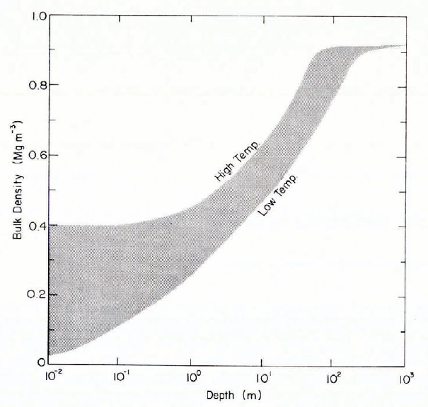
Fig. 3. General depth-density domain for snow deposits.
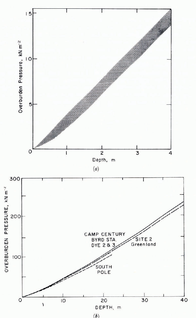
Fig. 4. Overburden pressure as a function of depth for snow deposits.
The bulk density of dry snow ρ can be expressed in dimensionless form as porosity n or void ratio r:

where ρ1 is the density of solid ice (0.917 Mg m-3).
Permeability
The permeability of snow is usually measured with an air permeameter, and until about 10 years ago it was customary to report an “air permeability" as the proportionality constant relating air flux rate to the gradient of head loss. A similar parameter, which is analogous to thermal conductivity in heat flow, is referred to elsewhere as “hydraulic conductivity" (using pressure gradient instead of heat-loss gradient), and the permeability of snow is now being reported as intrinsic permeability, or specific permeability k, i.e. the old “air permeability" multiplied by the dynamic viscosity of air (Reference ShimizuShimizu, 1970; Reference ColbeckColbeck, in press). The intrinsic permeability applies to movement of any fluid. In snow made up of equant grains, permeability appears to decrease exponentially with increasing density (inverse proportionality to porosity was suggested in earlier work), and it can be taken as increasing with the square of mean grain size (proportionality to d 1.63 was determined empirically in earlier work). For fine-grained compact snow, Reference ShimizuShimizu (1970) gave the relation
where k has the same dimensions as d 2 and ρs/ρwis the specific gravity of the snow (equal numerically to the usual expression of metric density in Mg m-3).
Impurities in Snow
"As pure as snow" may have been Hamlet’s idea of perfection, but virgin snow-and hoar frost-are usually contaminated to some degree, even in the remote central regions of Antarctica and Greenland. Some impurities are incorporated into precipitation during its formation and descent, while other kinds are deposited upon the snow surface as dry particles. A symposium on isotopes and impurities in snow and ice was held at Grenoble in 1975, and the forthcoming proceedings are expected to provide detailed information on some of the constituents listed below.
Stable isotopes
Natural snow crystals contain a small amount of H218O, and the ratio of H218O to the more common H216O (or the percentage difference) decreases slightly as the temperature of snow formation decreases (because of vapor-pressure differences). Variations in concentration of the oxygen isotope 18O can indicate seasonal and secular temperature variations at the site of snow formation, and rhythmic variations with depth in a snow deposit provide a means of dating the snow. Natural deuterium (2H) also occurs in otherwise uncontaminated snow.
Radioactive isotopes
Snow contains both natural radioisotopes and radioisotopes produced by human activity. Both types can be used for radioactive dating of “snow-ice" over long periods. Natural isotopes, which may be remnants of nucleogenesis or radionuclide products of cosmic-ray activity in the atmosphere, occur in ice molecules, in adsorbed and included air, in dissolved impurities, and in insoluble particles. “Unnatural" isotopes have been produced and injected into the atmosphere by employment and testing of nuclear weapons, and by nuclear power plants and their associated industries. Tritium (3H) occurs naturally in snow crystals, but the amounts found in deposited snow have been greatly increased since 1954 by weapons testing and nuclear industries. Other “natural" isotopes occurring in gases, dissolved impurities, and solid matter include radioactive isotopes of carbon, lead, argon, krypton, silicon, aluminum, chlorine, and manganese. Human activity with nuclear materials has provided additional sources for some of these, and has added goodies such as strontium and caesium isotopes.
Chemical impurities
Snow that has not been directly contaminated by local human activity receives chemical impurities from various sources. These include terrestrial dust and ocean spray; volcanic gases and dusts; plant emanations; combustion products from fossil fuels; fumes from industrial processes; dust and spray from road salts, pesticides, fertilizers; atmospheric modifications of any of the foregoing. Inorganic constituents that have been found in snow include Na, Ca, Mg, K (largely from sea salts), Al, Si, Ti, Fe, Pb, As, S (as SO2 and SO4), Se, I, CI, NH3, NO3 Mn, Cr, Cu, Zn, Cd, Hg, and various other trace elements. Organic constituents include hydrocarbons from combustion, organic synthesis, and other industrial processes, as well as hydrocarbons from plants, volcanoes and other natural sources. Traces of agricultural compounds such as DDT and PCB’s (polychlorinated biphenyls) are also found in snow.
Insoluble particles
Insoluble particles found in snow derive from various sources: wind-borne dust from terrestrial soils and rocks (including dust stirred up by agricultural and industrial activity); ash from volcanoes and industrial processes; extraterrestrial particles; plant pollens, plant fragments, phytoliths. Dust particles can become incorporated into precipitation during condensation, ice nucleation, and crystal growth. Heavy dust contamination occasionally gives rise to colored snowfalls (brown, red, yellow). Direct deposition of dust, ash, soot, or plant debris is frequently sufficient to stain the snow surface and form visible horizons at distinct levels within the snow-pack.
Living organisms
A variety of algae, fungi, bacteria, molds, and insects can live on snow surfaces, especially where temperatures are close to the melting point and light is plentiful. Very low temperatures arrest biological activity, but some micro-organisms remain viable after freezing. Organically tinted snows (red, green, yellow, and even blue) have been reported from various parts of the world; identifications and records have been published over a very long period by E. Kol (see Bibliography on cold regions science and technology, U.S. Gold Regions Research and Engineering Laboratory. Report 12, published annually, for references), and the physiology of algae on snow and ice has been studied by Reference FoggiFogg (1967) and Reference SmithSmith (1972). Particular algae species have been identified with particular colorations, but it seems that some species produce different colors at different stages of the life cycle, or else vary in color according to the available nutrients. Some of the species mentioned in connection with different colors include the following. Red snow: Chlamydomonas, Sphaerella, Protococcus, Scotiella. Green snow: Chlamydomonas, Raphidonema, Bracteococcus, Cryocystis, Scotiella, Ankistrodesmus, Stichococcus, Ochromonas. Yellow snow: Raphidonema, Scotiella (the bumper stickers reading “Don’t eat yellow snow” allude to other contaminants).
Acidity
Snow that has not been heavily contaminated is usually slightly acidic, with hydrogen ion concentrations in the range 10-4 to 10-7 mol l-1. On the ice sheets of Greenland and Antarctica, typical pH values for melt water are between 5 and 6, i.e. somewhat below the desirable minimum of 6 for drinking water.
Gases
Ice formed from snow fields contains small occluded air bubbles that entrap atmospheric gases representative of the time and place at which the bubbles became sealed. They contain, as well as oxygen and nitrogen, such things as CO2, CO, CH3 and Ar.
Selected Mechanical Properties of Snow
A comparatively recent review Reference Mellor(Mellor, [1975]) covered the general mechanical properties of snow, including surface friction, adhesion, and boundary shear stresses in fluidized snow. There is no point in repeating the work here, and only a few selected mechanical properties have been chosen for further discussion in this review.
Stress waves and strain waves in snow
A rapidly generated pulse of stress or strain propagates as an elastic wave when the amplitude is less than the failure stress or failure strain of the material. The wave attenuates with distance according to geometrical factors, and also by dissipative processes that are often referred to as internal friction.
Maximum sustainable amplitude for an elastic wave probably corresponds quite closely to the uniaxial strength of the snow for one-dimensional propagation in a long “bar”, and to the collapse strength of a “wide" layer for plane wave (or spherical wave) propagation (see figs 13 and 17 of Reference MellorMellor ([1975]), for an impression of general magnitudes).
The velocities of elastic dilatational waves (v ρ) and elastic shear waves (v s) depend on the elastic constants and the bulk density of the snow. In an infinite medium the body-wave velocities are:
where E is Young’s modulus, v is Poisson’s ratio, and ρ is density. Values of E and v for well-bonded dry snow were summarized earlier (Reference MellorMellor, [1975], fig. 2), but since E is itself a strong function of ρ, it is convenient to have a direct relation between velocity and snow density, as shown in Figure 5. Velocity also varies with the grain structure of the snow; during a period of sintering, both E and v increase with time as intergranular bonds develop, tending asymptotically to the limit values represented in Figure 5 (examples of data have been given by Reference MellorMellor (1964)). E does not vary much with temperature in dry snow (see Reference MellorMellor, [1975], fig. 2), and therefore v, being proportional to E½, is affected only slightly by temperature (about 0.1 % per degree). In addition to the body waves, a free boundary also carries a Rayleigh surface wave, which is sometimes referred to as “ground roll" in explosions technology. The velocity of the Rayleigh wave VR is less than v s, the ratio V R/V s decreasing with decrease of v (V R is likely to be about 7% less than Vs in dense snow).

Fig. 5. Velocities of elastic waves as junctions of snow density.
In an isotropic medium, elastic waves attenuate with distance by viscous damping and, unless they are plane waves, by geometric spreading. With spherical propagation from a point source, the energy per unit area of wave front I (which is proportional to the square of the wave amplitude A) follows an inverse-square decay because of spreading, and an exponential decay because of damping:

and
where r is the radius to the wave front and α is an attenuation coefficient that can be related to the “loss factor" of basic now mechanics (tan δ) by
Where f is frequency and λ is wavelength. The loss tangent varies with density, temperature and frequency (see Reference MellorMellor, [1975], figs 4-6); available data are probably too uncertain to depend on for working estimates of α, and direct measurements would be useful. It is to be expected that α will increase with increasing frequency (tan δ decreases as f increases).
Under an intense compressive impulse that exceeds the collapse strength of the snow, a “plastic wave" of inelastic strain is genera ted. The plastic wave front typically propagates at relatively low velocity, being preceded by a faster elastic wave of small amplitude that travels at sonic velocity for the undisturbed material. Ignoring effects of the elastic precursor and neglecting the entropy change due to the initial plastic compression, the pressure rise across the plastic wave front (density jump) can be estimated from the mechanical shock conditions, invoking conservation of mass and momentum:
where ρ is pressure, U is ρ particle velocity, U is plastic wave velocity, ρ is density, and subscripts 1 and 2 denote conditions before and after the jump. For the special case of initial impact between snow and a rigid plane surface, particle velocity u 2 relative to the impacting surface can be taken as zero, so that the expression for initial impact stress Δρ takes the form
In this expression u 1 is the impact velocity and (ρ 2-ρ 1)/ρ 1 or (-u 1/U) is volumetric strain. It should be noted that U and u 1 are of opposite sign.
In order to evaluate Equation (9) or Equation (10), it is necessary to have a kind of stress-strain relation that is known variously as a Rankine-Hugoniot equation of state, a Hugoniot, or a shock adiabat; it represents a locus of final states (end points of “ Rayleigh lines”) for shock compression, yielding appropriate relations for p, ρ, and u. In avalanche impact calculations, the Swiss practice is to take Δρ = ρ 1u 12 from rate of loss of momentum, and this is probably acceptable for a low-density snow. Reference MellorMellor (1968) evaluated Equation (10) by assuming a constant value of ρ 2 = 0.65 Mg m-3. The only known Hugoniot data for snow Reference Napadensky(Napadensky, 1964) were found to contain major errors (Reference MellorMellor, [1975]), but reinterpretation (Reference Mellor and VoightMellor, 1977[a]) yielded a relation between U/u 1 and ρ 1 or between ρ 2 and ρ 1 this relation being averaged for a range of values of u 1 from 10 to 60 m s-1. The Napadensky data have now been worked over again to obtain the relation shown in Figure 6, where U/u 1 is given as a function of ρ 1 with u 1 as parameter. It is hoped that new Hugoniot measurements will be made in the near future.

Fig. 6. Deduced relations between U/u 1, and ρ for various values of u 1. (Data from Reference NapadenskyNapadensky, 1964.)
There is a very strong attenuation of “plastic" waves with distance in snow, as is evident from the results of explosive cratering studies (see Reference MellorMellor, 1973). Measurements of explosive stress-wave amplitude with distance may not be completely accurate, but they serve to illustrate the strong attenuating properties of snow relative to other materials (Fig. 7). Combining the effects of geometrical spreading and internal dissipation, close-range attenuation of stress-wave amplitude is not far from an r -4 decay, and even near the elastic limit is it still approximately an r -3 decay.
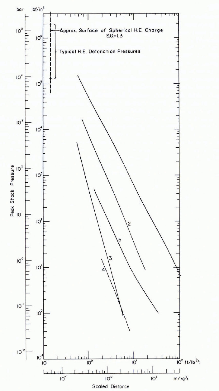
Fig. 7. Explosive stress-wave attenuation in snow and glacier ice compared with attenuation in rock, water, and air. (1) granite, (2) glacier ice, (3) ice-sheet snow, (4) seasonal snow, (5) air. The abscissa gives actual distance divided by the cube root of explosive charge weight, which amounts to an assumption of geometric similitude. (See Reference MellorMellor, 1968, Reference Mellor1972, for details of data sources.
Compressibility
Compressibility is of fundamental importance in snow mechanics and snow engineering, since most properties vary enormously with density, or specific volume. Under slow loading (e.g. gravity body forces), compressibility depends on the snow structure and the “static” strength properties. Under very rapid loading (inertial effects stress waves), compressibility depends mainly on density and velocity. Between these extremes, there is a range where compressibility is influenced by both static and inertial factors.
Ideas about slow densification under static loading do not seem to be at all clear On the one hand, snow is known to creep, and so densification is treated as a continuous time-dependent process, and viscosity coefficients are determined. On the other hand, addition of compressive load is known to produce a volumetric strain-rate that decays with time towards an asymptotic limit that is low enough for depth-density relations (or, more exactly, stress-porosity Footnote * relations) to be almost time-invariant and, allowing for temperature, quite similar from place to place, implying quasi-plastic behavior.
If the variation of volumetric strain with time under constant load is approximately exponential, the rate constant can be discussed in terms of a “half-life” for pseudo-equilibration between volumetric stress and strain (or density). If the half-life is short compared with the interval between successive additions of load, as it is near the surface in some seasonal snow covers, then application of continuous-creep theory could give misleading results; it would be simpler and perhaps more realistic to treat the compression as “instantaneous” (the formalism then becomes similar to elastic analysis—see Equation (30) and figure 15 of Reference MellorMellor, [1975]). By contrast, if the half-life is long compared with the interval between additions of load increments, as might be the case in the deeper layers of ice-sheet snow, then continuous creep theory of the type developed by Bader Reference Bader and Kuroiwa(Bader and Kuroiwa, 1962) would be applicable. In view of the stress dependence of ice viscosity, the rate constant or half-life for stress-density “equilibration” is likely to depend on both the snow density and the magnitude of the stress increment, as well as on the temperature. Densification rate for a compact of grains that deform by power-law creep has been treated formally by Reference Wilkinson and AshbyWilkinson and Ashby (1975), but the results would only be applicable to very dense snow or bubbly ice.

Fig. 15. ϵ″ as a function of frequency over the Debye dispersion range. Snow types given in the legend to Figure 14. (After Reference Yosida.Yosida and others, 1955; Reference Walt and MaxwellWatt and Maxwell, 1960.)
These distinctions could be important in engineering, especially where the primary interest is in strain and displacement, or in creep transients. They could also help to explain some of the creep-rate discrepancies that have been found between laboratory creep tests and field deductions from depth-density curves. More research is needed to sort out these effects: meanwhile, it is as well to treat with caution the “compactive viscosity” values that have been derived from application of continuous creep theory to low-density seasonal snow covers.
Compressibility effects at very high rates of loading are even more mystifying to the uninitiated (and maybe to the cognoscenti too). For example, it may not be immediately obvious why snow that can be penetrated by a lightly pushed pencil is able to stop and deform a bullet.
Inelastic compressive stress waves were discussed in the preceding section, and some compressibility characteristics were deduced for high-speed impact between snow and a rigid plane. The corresponding stress-density relationships for a range of impact velocities are shown in Figure 8. For very low densities, such as occur in dust avalanches and blizzards, sudden impact is not likely to happen, and the dynamic stress is perhaps better estimated as a stagnation pressure for fluid of appropriate density. Stagnation pressures for snow-free air are indicated on the zero-density axis of Figure 8. As density approaches the “ice” level, the elastic wave that was neglected in the treatment of “plastic” waves can reach large amplitudes, of approximate magnitude ρcu, where c is sonic velocity for material of density ρ. Elastic impact stresses for solid ice are marked on Figure 8, together with measured Hugoniot lines for ice. It can be seen that the potential amplitude of the elastic impact stress for very high velocity is limited by the compressibility of the ice.

Fig. 8. Deduced values of plane-wave impact stress as a function of density, with impact velocity as parameter. Stagnation pressures for snow of very low density are shown, as are elastic impact stresses for solid ice. Adiabats and isotherms for very high pressure are also shown.
At fairly low loading rates, say below impact velocities of 30 m s-1, the static strength of the snow probably has an influence. Uniaxial-strain compression tests have been made by Reference Abele and GowAbele and Gow (1975, Reference Abele and Gow1976) at displacement rates up to 0.4 m s-1, with temperatures from o to —413°C. A broad impression of the results is given in Figure 9, which indicates that stress levels developed at these relatively low deformation rates are comparable to impact stresses for higher-rate deformation in “unbonded” snow. Similar tests have recently been made on wet snow and snow slurry, but results are not yet available.
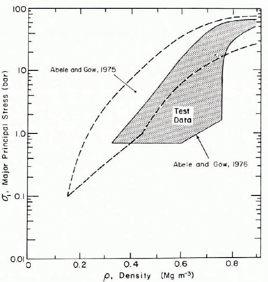
Fig. 9. Pressure—density relations for rapid compression of vented snow under uniaxial strain conditions. Reference Abele and GowAbele and Gow (1975, Reference Abele and Gow1976).
If an unvented volume of snow is compressed, or if there is compression over a wide area by a high-speed plane wave, then compression of the air in the pore spaces can create substantial resistance. The pressure rise Δρ a that is attributable solely to adiabatic compression of air in the pores is
where ρ 0 is original ambient air pressure and ρ 1 is ice density. Values for ρ 0 = 1 bar, ρ 1 = 0.1 Mg m-3 are plotted in Figure 8, and it can be seen that adiabatic air compression alone creates about as much resistance as 30 m s-1 impact of “vented” snow of ρ 1 = 0.3 Mg m-3.
Effect of volumetric strain on deviatoric strain
The relation between shear stress and shear strain-rate in snow is very strongly dependent on density (see Reference MellorMellor, [1975], fig. 16). The main interest in shearing tends to be in quasi-static creep problems, since at very high loading rate where there is rapid shearing and compression, the problems are usually treated as hydrodynamic ones, neglecting shear resistance. The range of interest is further narrowed by the fact that most problems involve both deviatoric stress and compressive bulk stress, often with gravity body forces playing a major part. In such cases it may be advantageous to by-pass the density-dependence of shear resistance, and seek instead a direct implicit relation between compressibility and shear resistance. This seems reasonable in snow where the grains have not become close packed, since both volumetric straining and shear straining involve shear displacement of grains relative to each other.
When well-settled snow lies on a wide uniform slope, and when near-surface complications arising from recent snowfall are ignored, the whole layer creeps downhill in such a way that a plane cross-section remains approximately plane. This phenomenon, which has fascinated the writer for many years Reference Mellor(Mellor, 1968, Reference Mellor[1975], Reference Mellor and Voight1977[a]), implies that resistance to shear deformation is proportional to shear stress or, since shear stress and normal stress are directly proportional, to normal stress or bulk stress. At the same time, it rules out assumptions of homogeneity for the snow-pack. The implications can be explored further by considering the equations for down-slope shear stress σxy, the corresponding shear strain-rate, the stress component normal to the slope plane σyy, the corresponding normal strain-rate, the shear viscosity μ and the bulk viscosity η (both the latter vary non-linearly with stress). The required equations (derived in Reference MellorMellor, 1968, p. 43—44) are
where the x and y directions are parallel and normal to the slope plane respectively, y being measured down from the surface, and ρ is the mean density from the surface down to depth y. Thus
or
From Figure 10 it appears that ![]() . The ratio η/μ should vary from 2/3 as ρ → o to α as ρ → ρi, but within the typical density range for settled seasonal snow-packs it is likely to be around unity or somewhat below (seeReference MellorMellor, 1968, p. 46, or Reference MellorMellor, 1975, equation 28 and fig. 12b). Thus, if (η/μ + 4/3)/2 ≈ 1, then
. The ratio η/μ should vary from 2/3 as ρ → o to α as ρ → ρi, but within the typical density range for settled seasonal snow-packs it is likely to be around unity or somewhat below (seeReference MellorMellor, 1968, p. 46, or Reference MellorMellor, 1975, equation 28 and fig. 12b). Thus, if (η/μ + 4/3)/2 ≈ 1, then ![]() This is not inconsistent with field observations of asymptotic values of
This is not inconsistent with field observations of asymptotic values of ![]() which seem to be of the order of 10-8 s-1. Unless care is exercised, there is some danger of circular argument with this kind of analysis, but at least it offers a possibility for obtaining useful numbers.
which seem to be of the order of 10-8 s-1. Unless care is exercised, there is some danger of circular argument with this kind of analysis, but at least it offers a possibility for obtaining useful numbers.
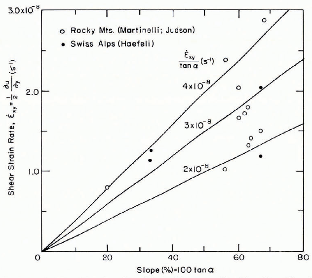
Fig. 10. Shear strain-rate as a function of slope for well-settled snow lying on a wide uniform slope. The arbitrarily drawn lines give different values of ![]() .
.
Specific energy for comminution
In analyzing processes such as cutting, boring, breaking, grinding, blasting, and excavating in solid materials, it is useful to define a specific energy consumption E s as the energy required to remove or comminute unit volume or unit mass (or power per unit comminution rate). Specific energy gives the relative efficiencies of different processes in a given material, and it also characterizes material properties with respect to a given process. In principle, specific energy can be referred to the energy required to create new surfaces and to the specific area of the comminuted product, or ultimately to the surface free energy of the material. However, for practical purposes it is better to refer to a more direct standard, and it has been shown that for typical brittle materials the specific energy for breakage in a conventional uniaxial compression test provides such a standard Reference Mellor(Mellor, 1972). If E s is expressed as energy per unit volume it has the dimensions of stress, and it can be normalized with respect to the uniaxial compressive strength (σc) of the material under consideration. For rocks and frozen soils that are not strongly anisotropic, as well as for polycrystalline ice, E s for breaking in a uniaxial test is approximately 10-3σc, which is comparable to the specific energy of a good stone crusher. However, for typical cutting and boring processes applied to rocks, frozen soils and ice, E s/σc is in the range 10 to 0.1 (Reference Mellor, Seltmann and SplettstoesserMellor and Sellmann, 1976; Reference Mellor, Hawkes, Lane and GarfieldMellor and Hawkes, 1972[a], Reference Mellor and Hawkes[b]), perhaps extending somewhat below 0.1 under favorable experimental conditions (Reference MellorMellor, 1977 [b]).
Measurements have been made on snow to determine the “work of disaggregation”, i.e. the specific energy for breaking a snow compact into its constituent grains. Data obtained by Bender (reported by Reference ButkovichButkovich, 1956) are remarkable in that E s/σc ≈ 2 × 10 -3 for disaggregation of dense dry snow by a grinding drum. Reference CroceCroce (1958) made measurements with a different kind of cutting device and obtained results that seem to be very much higher than the comparable Bender data. (Guessing a value of σc from Croce’s stated value of ρ = 0.3 Mg m-3, E s/σe might be in the range 0.01 to 1.0.) It has been noted that rammsonde resistance represents a specific energy for disaggregation and displacement Reference Mellor(Mellor, [1975]); in moderately dense dry snow E s/σc seems to be between 1.0 and 0.1 for this process, although it is greater than 1.0 for high-density snow.
There is obviously a good deal of uncertainty about the specific energy for cutting, breaking and disaggregating snow, and new measurements seem overdue. E s is needed for full evaluation of snow plows, over-snow vehicles, and excavating machines, and it is relevant to the energetics of avalanche motion.
Thermal Properties of Snow
Heat capacity or specific heat
The specific heat c of a material is the heat required to produce unit temperature rise in unit mass, at either constant pressure or constant volume. In snow, the requirements for heating air and water vapor in the interstices are very small, so that for most practical purposes the specific heat of snow is the same as the specific heat of ice, which varies with temperature and with purity. The effects of high specific surface area and grain surface curvature in snow are negligible.
Apparent specific heat c a is given as a function of temperature and impurity concentration by an empirical equation derived by Reference Dickinson and OsborneDickinson and Osborne (1915):
where θ is in °C (making the second term negative), and d is the initial freezing temperature in °C (making the final term positive). For pure ice the last term is dropped. This determination was made at temperatures down to —40°C and for values of d from —5 × 10⁻⁵ to —1.25 × 10⁻³ °C. The effect of temperature over a wide range (-263 to —3°C) was determined by Reference Giauque and StoutGiauque and Stout (1936), and later studies by Flubacher and others (1960) supplemented the data for extremely low temperatures (2 to 27 K). Figure 11 shows the effect of temperature down to absolute zero.

Fig. 11. Specific heat of ice as a function of temperature. (Giauque and Stout, 1936)
These determinations are for ordinary hexagonal ice at constant pressure (cρ). Calculated values for specific heat at constant volume (cv) are approximately 3% lower at 0°C, and the difference between cρ cρ and cv decreases as temperature decreases Reference Hobbs(Hobbs, 1974), making the distinction unimportant for most practical purposes.
For simple calculations that do not call for a high degree of accuracy, it is convenient to remember and use a rounded value of 0.5, either cal g-1 deg-1 or Btu lb-1 °F-1, risking heresy charges from the SI priesthood (0.505 7 cal g-1 deg-1 = 2.12 J g-1 K-1).
Latent heat of fusion and sublimation
The latent heat of snow is almost invariably taken as identical to the corresponding latent heat of ice. Precise values for pure ice at 0°C and standard atmospheric pressure are:
latent heat of fusion = 79.67 cal g-1 = 333.5 J g-1,
latent heat of sublimation = 678.0 cal g-1 = 2 838 J g-1.
The latent heat of sublimation at a given temperature is generally taken as the sum of the latent heats of fusion and vaporization. The latent heat of fusion for ice decreases with decreasing temperature, while the latent heats of vaporization and sublimation increase with decreasing temperature. Table I gives values derived by de Reference Forcrand, Gay and WashburnForcrand and Gay (1929) and Reference Dickinson and OsborneDickinson and Osborne (1915), as listed by Reference DorseyDorsey (1940), together with values calculated from the Goff-Gratch formula, as listed in the Smithsonian Meteorological Tables Reference List(List, 1951).
Table I. Latent Heat of Ice

Thermal conductivity
In one-dimensional heat flow, the thermal conductivity is the heat flux q divided by the temperature gradient (dθ/dz), i.e. it is the proportionality constant of the Fourier equation for steady-state unidirectional heat flow:
In dielectric solids in general, and also presumably in solid ice, thermal conductivity is attributed to lattice vibrations and phonon diffusion in the crystals. In non-aspirated dry snow the heat transfer process is considerably more complicated, involving (a) conduction in the network of ice grains and bonds, (b) conduction across air spaces or pores, (c) convection and radiation across pores (probably negligible), and (d) vapor diffusion through the voids.
Because of these complications, the thermal conductivity of snow is expressed as an effective thermal conductivity k e, which is intended to embrace all of the heat-transfer processes. However, measured values of k e depend to some extent on the measuring method (both transient and steady-state methods have been used), and there is no guarantee that the thermal situation in a practical problem will correspond to the situation under which a particular set of values of k e were measured.
The effective thermal conductivity of snow depends very much on bulk density ρ, varying by art order of magnitude for the density range from 0.1 to 0.6 Mg m-3 (Fig. 12). Results of the various experimenters are shown on logarithmic scales in Figure 12, which also gives representative values for ice, thus indicating the end point to which the snow data ought to extrapolate. Most experimenters have given empirical expressions which show k e proportional to ρ or ρ 2, or else k e as a polynomial in ρ. Japanese workers have preferred logarithmic expressions which seem to fit the snow data well, although the constants perhaps need adjustment to fit the upper boundary condition for ice. Overall, the experimental values for k e vary by a factor of 2 at any given density, and highly anomalous results have turned up in some of the Japanese work on low-density snow.
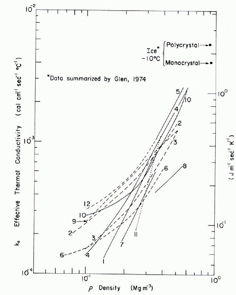
Fig. 12. Effective thermal conductivity of snow as a function of density.
Data from:
1. Abels, 1894.
2. Janson, 1901.
3. Van Dusen, 1929.
4. Devaux, 1933.
5. Kondrareva, 1945.
7. Bracht, 1949.
8. Sulakvelidze, 1958.
9. Proskuriakao.
10. Reference Pitman and ZuckermanPitman and Zuckerman, 1967 (-5°C).
12. Kobayashi and Ishida, 1974.
Calculated values of k e for snow and bubbly ice were obtained by Reference SchwerdtfegerSchwerdtfeger (1963) from structural models analogous to the classical Maxwell models for electrical conductivity in two-phase media. Considering only conduction in ice and in air, and taking reasonable rounded values for the conductivities of ice and air, a composite curve for k e in snow and bubbly ice was obtained. This curve, which plots almost as a straight line against logarithmic axes, coincides more or less with the upper limit of the results shown in Figure 12. Schwerdtfeger also determined an extreme lower-bound relation for ice particles dispersed in air; this curve falls well below all of the data of Figure 12. One outcome of Schwerdtfeger’s analysis is a formal indication that the conductivity of still air does not have much effect on k e for densities higher than about 0.15 Mg m-3.
A more detailed theoretical and experimental study was made by Reference Pitman and ZuckermanPitman and Zuckerman (1967). Three different models were considered, vapor diffusion was taken into account, and temperature was a variable in both experiments and analyses. The starting point was a sphere model for conductivity in porous media proposed by Reference WoodsideWoodside (1958), and directly applicable only for porosities below 0.48 (snow densities greater than 0.48 Mg m-3). A switch of gas and solid parts of the model was used as a modification for low snow densities. A second model consisted of a statistical mixture of series and parallel laminar basic cells, following an electrical conductivity model proposed by Reference Wyllie and SouthwickWyllie and Southwick (1954). A third model was a modification of the Woodside model that gave continuous ice pathways between spherical grains. Using a parameter chosen arbitrarily to provide best fit, the third model gave good agreement with the experimental data for densities from 0.1 to 0.4 Mg m-3 and temperatures of —5 and —27°C. However, there is some question about the value chosen for the diffusion coefficient. (The value for water vapor through air, 22 m2 s-1, was taken, but effective values for diffusion in snow are 3 to 4 times greater—see section on vapor diffusion.)
If the conductivity of motionless air (about 5.5 × 10⁻³ cal cm-1 s-1 deg-1) is relatively unimportant, and if vapor diffusion is ignored, then it might be expected that the temperature dependence of thermal conductivity would parallel that of ice. At temperatures above 120 K, the thermal conductivity of ice increases approximately as the inverse of absolute temperature, so that there is not much temperature sensitivity in the common range of environmental temperatures, say down to —30°C (see Reference FletcherFletcher, 1970; Reference GlenGlen, 1974; Reference HobbsHobbs, 1974; Reference KlingerKlinger, 1975). However, both analytical and experimental results by Pitman and Zuckerman (Fig. 13) show the thermal conductivity of snow decreasing with decreasing temperature. This suggests that, while air conductivity may be unimportant, vapor diffusion in the pores is very significant (as will be shown shortly).
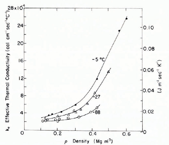
Fig. 13. Effective thermal conductivity as a function of density for three different temperatures. (From Pitman and Zuckerman, 1968.)
In many engineering applications, it is neither necessary nor desirable to worry about the finer details or complications of k e, although it is as well to know they exist. For problems involving dense snow or bubbly ice, it may be sufficient to take k e as proportional to ρ 2, adopting suitable reference values as being either representative or conservative, as circumstances dictate.
Thermal diffusivity
The thermal diffusivity a is the coefficient of the general heat-conduction equation. It is the thermal conductivity divided by the product of density and specific heat (“volumetric specific heat”):
Since c is invariant with density, α varies less with ρ than does k e; for dense snow and bubbly ice, a is approximately proportional to ρ. According to the data of Pitman and Zuckerman (1968), k e decreases with decreasing temperature. At the same time, c decreases as temperature decreases. Thus α should be relatively insensitive to temperature change at ordinary environmental temperatures. The same conclusion was reached from different premises by Reference Yen.Yen (1969).
Heat transfer by vapor diffusion
Saturation vapor pressure increases with temperature, so that a temperature gradient in snow sets up a gradient of vapor pressure ρ, and molecules are transferred from grain to grain, carrying along latent heat. In the diffusion equation for vapor pressure there is a diffusion coefficient D that is analogous to the thermal diffusivity α in the diffusion equation for energy or heat conduction. In one-dimensional steady-state diffusion, Fick’s law gives D as the constant equal to the mass flux divided by the concentration gradient. The rate of heat transfer due to one-dimensional steady-state vapor diffusion is given by Equation (20) when k is replaced by an equivalent thermal conductivity for vapor diffusion k v. The relation between k v and the effective diffusion coefficient D e is:
where β is the rate of change of vapor density of ice with temperature and L s is the latent heat of sublimation for ice.
Reference Yosida.Yosida and others (1955) measured D e for snow specimens ranging in density from 0.08 to 0.51 Mg m-3; D e ranged from 70 to 100 mm2 s-1 (mean 85 mm2 s-1), with no apparent relation to density. Reference YenYen (1963, Reference Yen1965[a], Reference Yen.[b], Reference Yen.1969) carried out forced convection experiments (see next section) and from the results found a no-flow lower limit for D e of 65 mm2 s-1. The same value was obtained with ρ ranging from 0.38 to 0.47 Mg m-3, and from 0.50 to 0.59 Mg m-3. Reference Yen.Yen (1969) believed that the difference between his value and those of Yosida was partly due to the lower temperature range used in his experiments.
These values of D e are much higher than the accepted values for the diffusion coefficient of water vapor in air (≈ 22 mm2 s-1 at 0°C and atmospheric pressure). Possible reasons for the difference include local intensification of the temperature gradient across air spaces, and shortening of the effective diffusion path by grain-to-grain sublimation transfer.
Taking L s = 676 cal g-1 (2.83 kJ g-1), β = 0.39 × 10⁻⁶ Mg m-3 deg-1, and D = 75 mm2 s-1 (mean of the Yosida and Yen results), the effective thermal conductivity attributable to vapor diffusion is k v ≈ 2 × 10⁻⁴ cal cm-1 s-1 der-1 (≈ 0.08 J m-1 s-1 K-1). This implies that at ρ = 0.25 Mg m-3, vapor diffusion might account for about half the total heat transfer, while at ρ = 0.1 Mg m-3, vapor diffusion dominates the heat-transfer process.
Heat transfer and vapor transport with forced convection
When there is a difference of air pressure across a mass of snow, there is forced convection through the pore structure, with consequent intensification of heat transfer and vapor transport. Forced convection was an important consideration in the design and operation of large under-snow installations in Greenland and Antarctica, where air for ventilation and cooling was drawn from the pores of the surrounding snow mass (most notably in the air-blast cooler tunnel of the Camp Century nuclear power plant).
Thermal effects of forced convection were studied theoretically and experimentally by Reference YenYen (1962, Reference Yen1963, Reference Yen1965[a], Reference Yen.[B], Reference Yen.1969), and effective values of thermal conductivity k e′ and diffusion coefficient D e′ were determined as functions of the mass flow rate of air G. For the density range 0.38 to 0.47 Mg m-3, and with flow rates in the range 1 × 10⁻³ to 4 × 10⁻³ g cm-2 s-1, empirical expressions for the effective values were
These results cover tests on specimens with four different particle sizes ranging from 0.7 to 2.2 mm. For the density range 0.50 to 0.59 Mg m-3, and for flow rates G ranging from 5 × 10⁻⁴ to 3.2 × 10⁻³ g cm-2 s-1, the empirical expressions for k e′ and D e′ were
The no-flow lower limits of these expressions have already been mentioned in the section on vapor diffusion.
Thermal strain
Thermal expansion coefficients do not seem to have been measured for snow. In dense snow, where there is close packing of ice grains, the thermal expansion ought to approximate that for solid ice. The coefficient of linear expansion for ice is approximately 5 × 10⁻⁵ deg-1 at 0°C, and it decreases almost linearly with temperature to about 2 × 10⁻⁵ deg-1 at —150 °C (it becomes negative around —200°C). In snow of low density, the expansion coefficient is likely to be lower than the ice value (with unconnected ice grains dispersed in air, there would be no thermal expansion of a vented control volume).
Electrical Properties of Snow
Dielectric properties
The dielectric properties of dry snow are closely related to those of solid ice (they should be calculable from ice properties with a suitable model), and therefore it is convenient to refer first to the dielectric properties of ice itself.
Terminology
The complex dielectric constant, or complex relative permittivity, ϵ* is
where the real part ε ′ is the dielectric constant or relative permittivity, and the imaginary part ε ″ is the dielectric loss or relative loss factor. The ratio ε ″/ε ′ is equal to the loss tangent, tan δ, where the loss angle δ is the phase angle between the loss current and charging current vectors. ε ′ and ε ″ are functions of frequency and temperature; the zero frequency value of ε ′ is the static relative permittivity ε s′ (or ε s), and the high frequency value ε ∞′ (or ε ∞) is the high frequency (ω ≫ 1/τ) relative permittivity. ε′—ε ∞′ is the dispersion. For a polarization that has a single dielectric relaxation time τ, the dependence of ε′ and ε″ on (angular) frequency ω can be described by the Debye dispersion equations:
Elimination of τ from this pair of equations gives a relation between ε ′ and ε ″ that plots as a semi-circle of diameter ε s —ε ∞ centered at ½(εs + ε∞) on the ε″ axis (Cole-Cole plot). The apparent a.c. conductivity σ′ (real part of complex conductivity) is
where ε 0 is the absolute permittivity in vacuum.
Permittivity of ice
For pure ice, ε s is approximately too at ordinary environmental temperatures; from a value that is probably somewhat below too at 0°C, it increases with decreasing temperature at roughly 0.4% per degree (ε s is approximately proportional to 1/T at ordinary temperatures; over a wider range, the Curie-Weiss law gives better representation—see Reference HobbsHobbs (1974)). As frequency increases, there is a well-defined Debye dispersion (there may also be other dispersions) and ε ′ falls rapidly to a high frequency value of ε ∞ ≈ 3.2, which is only slightly temperature-dependent (ε ∞ appears to decrease with decreasing temperature at about 0.04% per degree down to —25°C). This drop takes place in a two-decade frequency range that is centered about the frequency f where ε ″ is a maximum, i.e. where ωτ = 1 and f = ω/2π = 1/2πτ. The relaxation time τ for the Debye dispersion is approximately 2 × 10⁻⁵ s (f ≈ 104 Hz) at 0°C, and it increases to about 10-3 s (f ≈ 102 Hz) at —4.0°C in accordance with the Arrhenius relation (with activation energy of about 0.58 eV). By contrast, ε s for liquid water at 0°C is about 88, and the dispersion frequency is about 1011 Hz (so that there is a large difference between ε ∞ for water and ice over much of the radio and microwave range). for ice stays approximately constant as frequency increases up to the infrared range (1012-1014 Hz), where there are molecular absorption bands, and ε ′ then drops to 1.7 (square of the refractive index) for the optical (visible) range (1014-1015 Hz). There is further absorption in the ultra-violet, with a final drop to ε ′ = 1 for the X-ray range.
The underlying physics is discussed by Reference Eisenberg and KauzmannEisenberg and Kauzman (1969), Fletcher (1970), Reference ParenParen (unpublished), Reference HobbsHobbs (1974), Reference GlenGlen (1974), Reference Glen and ParenGlen and Paren (1975); detailed reference lists are given by these authors.
Dielectric loss in ice
Dielectric loss in ice is often discussed in terms of apparent conductivity σ′, since ε ″ = σ′/(ω ε 0), or tan δ = σ′/(w ε 0ε ′). Low-frequency conductivity (or bulk d.c. conductivity) for ice of high purity is of the order of 10-8 to 10-7 Ω-1 m-1 around — 10°C, and it decreases with decreasing temperature over the ordinary environmental range at the rate of a few per cent per degree (Arrhenius relation with activation energy of about 0.3 to 0.4 eV). Above the Debye dispersion frequency, which increases with temperature as already mentioned, a’ typically increases by about two orders of magnitude, giving high-frequency values σ∞ of the order of 10-5 Ω-1 m-1 at temperatures around — 10°C. The high frequency conductivity σ∞ then stays approximately constant as frequency increases up to 108 Hz; σ∞ decreases with decreasing temperature at a few per cent per degree (Arrhenius relation with activation energy 0.2 to 0.6 eV). Over the high-frequency range where σ∞ is effectively invariant with frequency, ε ″ must obviously be inversely proportional to ω, and since ε ′ is approximately constant in the same range, tan δ will also be inversely proportional to w (or f). Above 108 Hz, σ′ increases again, reaching values more than an order of magnitude higher than σ∞ at 1010 Hz and higher frequencies. Dielectric loss can also be expressed in terms of wave attenuation with distance; in the σ∞ range, where tan δ < 10-1, the attenuation α is
In the HF/VHF range (107-108 Hz), α for pure ice is about 0.07 dB/m at 0°C, falling non-linearly to about 0.01 dB/m at —25°C Reference Johari and Gharette(Johari and Charette, 1975).
Dielectric properties of snow
Dry snow of moderately high density consists of equant particles and air-filled voids, while very dense snow that is nearing the transition from permeable snow to impermeable porous ice consists of an ice matrix with equant air voids or bubbles. With this kind of structure, a number of relatively simple models for the dielectric behavior of two-component mixtures are potentially applicable. However, equations derived from such models should be applied with caution, having due regard for the assumptions, explicit, implicit, or illicit, that underlie their derivations. A detailed discussion of dielectric mixture models applied to snow is given by Reference ParenParen (unpublished), and applications are given by Reference Glen and ParenGlen and Paren (1975).
Wet snow, which is a three-component mixture of ice, water and air, is more complicated. Nevertheless, Sweeney and Colbeck (1974) had some success in applying a mixture model to unsaturated wet snow in the microwave frequency range, as did Reference Ambach and DcnothAmbach and Denoth (1972) at 20 MHz.
Dielectric dispersion in snow
Figure 14 summarizes measured values of the relative permittivity ε ′ through the frequency range where Debye dispersion takes place. The frequency corresponding to the relaxation time for ice at 0°C is approximately 104 Hz, and it appears that relaxation frequencies for snow may be systematically higher. Measured values of the relative loss factor ε ″ are shown as a function of frequency for the dispersion region in Figure 15. Figure 16 shows the relative constancy of ε ′ (or ε ∞) from MF radio frequencies up to the radar K band (106-1010 Hz). The dielectric properties of snow tend to be characterized chiefly by bulk density and temperature, but Figure 17, which gives ε ′ and ε ″ as functions of frequency through the Debye dispersion region for sintering snow, shows very clearly that there can be drastic variations of dielectric properties at constant density and constant temperature.

Fig. 14. ε′ as a function of frequency over the Debye dispersion range. (After Yosida and others, 5955; Watt and Maxwell, 5960.) Note: r and 4: Watt and Maxwell. 2, 3 and 5-12: Yosida and others.
1. Wet snow, 0°C, p = “compact”.
2. Wet snow, 0°C, p = 0.38 Mg m-3, chlorine 25 mg/kg.
3. —7°C, p = 0.38 Mg m-3, chlorine 25 mg/kg.
4. Wet snow, 0°C, p = 0.6 Mg m-3.
5. Granular snow, — 4°C, p = 0.4f Mg M-3, chlorine 12.5 mg/kg (2-4 mm grains; in condenser 24 h).
6. Granular (measured immediately).
7. —3°C, p = 0.40 Mg m-3, chlorine 35 mg/kg (in condenser 24 h).
8. —3C, p = 0.40 Mg m-3, chlorine 35 mg/kg (measured immediately).
9. New snow with dendritic crystals, — 1°C, p = 0.25 Mg m-3, chlorine 15 mg/kg.
10. New snow with denditic crystals, — 1°C, p = 0.095 Mg m-3, chlorine 15 mg/kg.
11. New snow with dendritic crystals, — 1°C, p = 0.13 Mg m-3, chlorine 15 mg/kg.
12. Artificial pure snow, —8.5°C, p = 0.29 Mg m3.

Fig. 16. ϵ ’ as a function of frequency, from MF radio frequencies up to the radar K band. (After Reference YoshinoYoshino, 1961.)
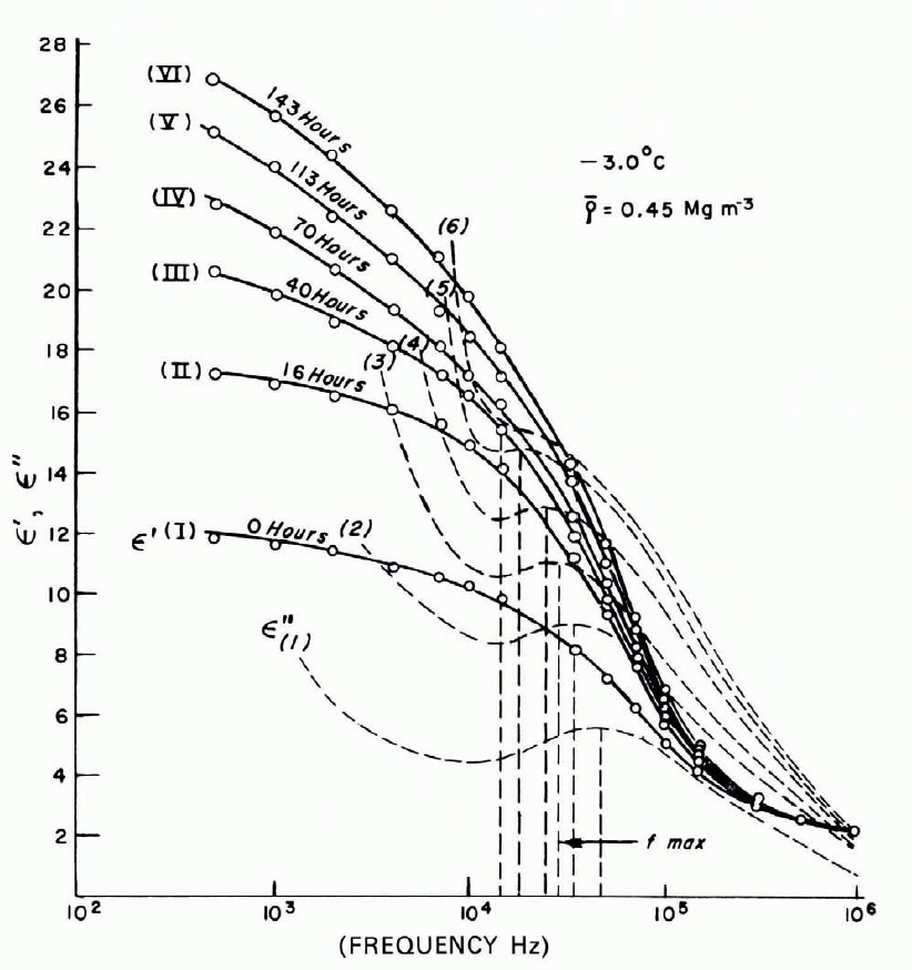
Fig. 17. ϵ ′ and ϵ ″ as functions of frequency for sintering snow, with time as parameter. (After Reference Bader and KuroiwaBader and Kuroiwa, 1962.)
Permittivity of snow
Figure 18 shows measured values of ε s and ε ∞ as functions of snow density. For ε s, the results of Reference Bader and KuroiwaBader and Kuroiwa (1962) and Reference KeelerKeeler (1969) are in general agreement; temperature ranges for the two data sets were o to —7°C and —3 to — 10°C, respectively. For ε ∞, the results of Reference Bader and KuroiwaBader and Kuroiwa (1962), Reference cummingCumming (1952), and Reference Ambach and DcnothAmbach and Denoth (1972) are in good agreement. The Cumming curve (for —18°C) is virtually coincident with the curve representing values calculated according to the simple Looyenga model. Values of ε ∞ obtained by Reference YoshinoYoshino (1961) for Antarctic snow at —18 and 36°C are much lower than the other values, and if correct they perhaps reflect the effects of poor bond development in very cold snow. The break in slope at ρ ≈ 0.55 Mg m-3 appears significant, since this represents the closest grain packing that can easily be achieved by rearrangement of grains (density-dependence of some other properties is also discontinuous at this density).
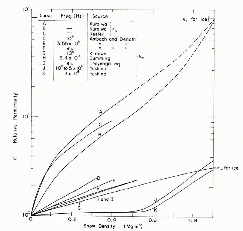
Fig. 18. Relations between ϵs and ρ and between ϵ∞ and ρ.
The high-frequency permittivity of wet snow increases as the liquid-water content increases, as would be expected from the large difference between permittivities of ice and water in this frequency range. Figure 19 gives measurements by Reference Sweeny and ColbeckSweeny and Colbeck (1974), showing ε ′ at 6 × 10⁹ Hz increasing more or less linearly with the degree of saturation in snow of porosity 0.4 (dry density 0.55 Mg m-3). Reference Ambach and DcnothAmbach and Denoth (1972) found a linear relation between water content and the difference between wet and dry permittivities. Having found a linear relation between ε ∞, and density ρ for dry snow, they were able to express [(ε ∞)wet- (ε ∞) dry] as [(ε ∞)wet - 1 —2.22ρ], where ρ is in Mg m-3 (Fig. 20). Some earlier results in similar form are shown in Figure 21.
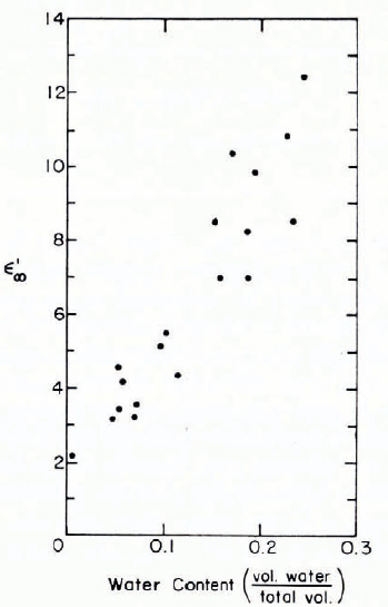
Fig. 19. ϵ∞ (at 6 × 10⁹ Hz) plotted against liquid-water content for wet snow. (After Reference Sweeny and ColbeckSweeny and Colbeck, 1974.)

Fig. 20. Difference of wet and dry permittivities plotted against liquid-water content for wet snow. (After Reference Ambach and DcnothAmbach and Denoth, 1972.)
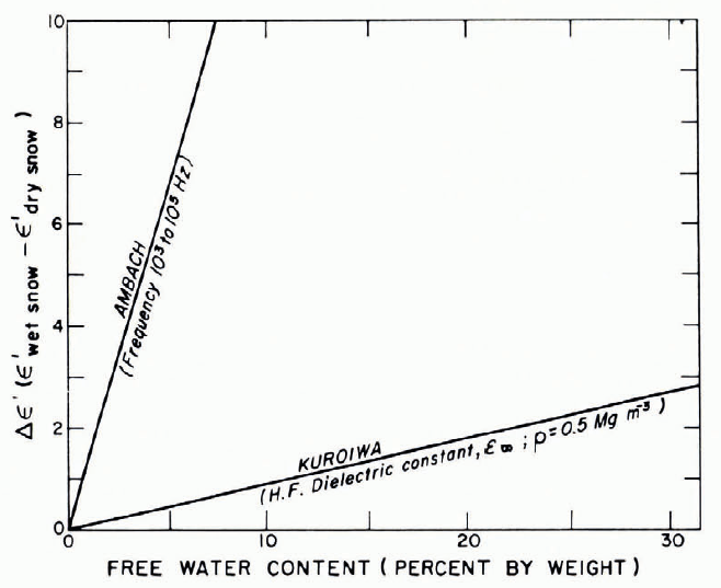
Fig. 21. Difference of wet and dry permittivities plotted against liquid-water content for wet snow. (Data from Reference AmbachAmbach, 1958; Reference Bader and KuroiwaBader and Kuroiwa, 1962.)
Dielectric loss in snow
Figure 22 gives some data for the variation of tan δ with frequency. The results for snow of ρ ≈ 0.3 Mg m-3 at frequencies above the Debye dispersion show tan δ decreasing with f at significant rates, tan δ being roughly inversely proportional to f ½ from 105 to 107 Hz, and to f from 108 to 1010 Hz. Yoshino’s results show a distinct change in frequency dependence around 108 Hz, and a rather weak density dependence.
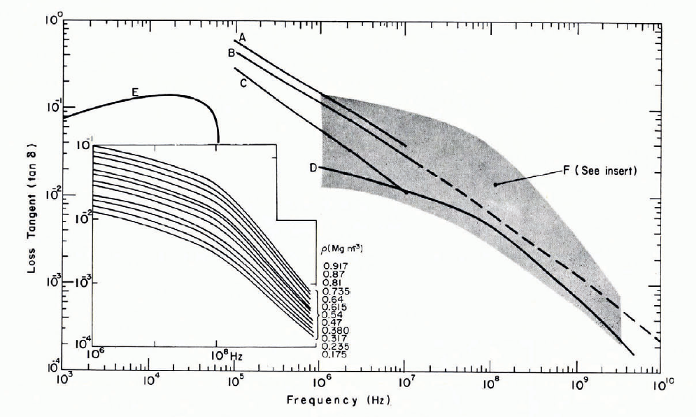
Fig. 22. Loss tangent as a function of frequency from 103 to 1010 Hz.
A. Kuroiwa, p = 0.3 Mg m-3, θ = —4°C.
B. Kuroiwa (broken line joins Kuroiwa’s data to Cumming’s data for 1010 Hz), p = 0.3 Mg m-3, θ = —12°C.
C. Kuroiwa, p = 0.3 Mg m-3, θ = —22°C.
D. Yoshino, p = 0.32 Mg m-3, θ = —18 to —36°C.
E. Ambach.
F. Yoshino, θ = —18 to —36°C.
The density dependence of tan δ in the frequency range from 106 to 1010 Hz is shown in Figure 23; tan δ increases by about an order of magnitude through the complete transition from low-density snow to impermeable ice.

Fig. 23. Loss tangent as a function of density. (A-E, Reference YoshinoYoshino, 1961; F-J, Cumming, 1952.)
The temperature dependence of tan δ at 103 Hz is illustrated in Figure 24, which shows a significant increase with increasing temperature above —10°C, but not much variation at lower temperatures.
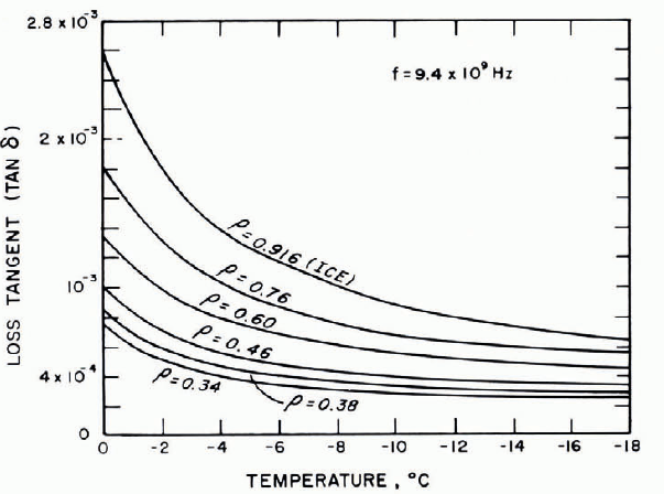
Fig. 24. Loss tangent as a function of temperature, with density as parameter. (After Cumming, 1952.)
In Figure 25 tan δ is shown as a function of water content for wet snow at a frequency of approximately 1010 Hz. In samples of both moderately dense and very dense snow there is a strong increase of tan δ as the water content increases from zero to less than 2%. Figure 26 gives another example of data for a similar frequency (6 × 10⁹ Hz).
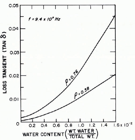
Fig. 25. Loss tangent as a function of liquid-water content for wet snow. (After Cumming, 1952.)

Fig. 26. Loss tangent plotted against liquid-water content for wet snow. (After Reference Sweeny and ColbeckSweeny and Colbeck, 1974.)
The apparent a.c. conductivity, or dielectric conductivity, is 5.56 × 10⁻¹¹f ε ″ Ω-1 when f is in Hertz.
D.C. conductivity of snow
Reported values of d.c. conductivity for snow vary considerably, partly because there really is wide variation, and partly because there are measurement problems. Reference ParenParen (unpublished) lists results of various field measurements (Reference AndrieuxAndrieux, unpublished; Reference Chaillou and VallonChaillou and Vallon, 1964; Reference HochsteinHochstein, 1965; Reference Hochstein and RiskHochstein and Risk, 1967[a], Reference Hochstein and Risk[b]) for “cold” snow of unspecified density; in these studies, d.c. conductivity stayed within a surprisingly narrow range, from 9 × 10⁻⁷ to 4 × 10⁻⁶ Ω-1 m-1. Paren also derived d.c. conductivities of 10-8 to 3.6 × 10⁻⁷ Ω-1 m-1 from Keeler’s (1969) dielectric measurements on dry seasonal snow (density 0.08 to 0.40 Mg m-3, temperature —3 to —10°C). He also derived d.c. conductivity values from his own low-frequency field measurements, obtaining for temperatures above —10°C values of 10-6 Ω-1 m-1 for ρ ≈ 0.2 Mg m-3, and 4.8 × 10⁻⁶ for ρ ≈ 0.4 Mg m-3. In an earlier compilation, Reference MellorMellor (1964) gave results (from Reference KoppKopp, 1962; Reference Meyer and RöthlisbergerMeyer and Röthlisberger, 1962; Reference ShimodaShimoda, 1941; Vögtli, unpublished; Reference TsudaTsuda, 1951) that lay mostly in the range 10-8 to 10-5 Ω-1 m-1, without much correlation with density for the results overall. An exception to the last statement has to be made for the Kopp data, which show d.c. conductivity increasing by almost three orders of magnitude as density increases from 0.13 to 0.57 Mg m-3 (approximate linear relation between log σ and ρ).
Reference KoppKopp’s (1962) results show a strong temperature dependence for d.c. conductivity (Fig. 27); conductivity increases by three orders of magnitude as temperature increases from —60 to — 10°C, and there is a sharper increase at temperatures above —10°C. The Reference TsudaTsuda, 1951 data (Fig. 28) show the rapid increase in conductivity that occurs as free-water content increases in “warm” snow.

Fig. 27. D.C. conductivity as a function of temperature, with density as parameter. (After Reference KoppKopp, 1962.)
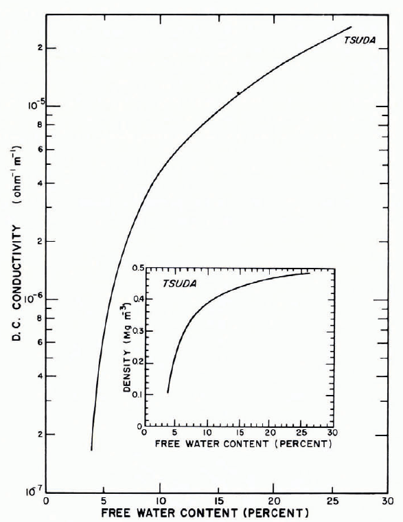
Fig. 28. D.C. conductivity as a function of liquid-water content for wet snow. (After Reference TsudaTsuda, 1951.)
Thermoelectric effect
Particles or prisms of pure ice that have a temperature gradient develop a corresponding electrical potential gradient, with the warm end negative and the cold end positive (relatively). As long as temperatures are below —10°C, the potential difference is approximately proportional to the temperature difference, at about 1.5 to 3.5 mV deg-1 (this millivolt per degree ratio is referred to as “thermoelectric power”). Small concentrations of dissolved impurities have been found to decrease the “thermoelectric power” (NaCl) and also to increase it slightly (HF, CO2); higher concentrations of HF and NH4OH (or NH3) have produced decreases from a peak of about 4 mV deg-1 that occurred at a melt-water pH of 7.2, with the thermoelectric power changing sign (warm end becoming positive) above a melt-water pH of 7.8 (NH3 contamination). When some part of the (“pure”) ice is warmer than —10°C, the thermoelectric power departs from the approximately constant value found for low mean temperatures, but there are conflicting reports on whether it increases or decreases. A brief contact between two pieces of ice that have different temperatures creates a potential difference and charge transfer. Maximum potential difference varies with contact time, peaking at about 7 ms, and it increases with impact velocity around the 0.1 m s-1 range. Thermoelectric effects are discussed in detail by Reference HobbsHobbs (1974), who gives relevant references.
Particles of falling snow and blowing snow can be expected to have complicated thermoelectric behavior. They have high, and variable, specific surface areas (which is probably important at temperatures above —10°C), they move through atmospheric temperature gradients and sometimes rotate at the same time, they sometimes collide, and they undergo surface ablation or accretion.
Electrical charge on falling snow and blowing snow
Particles of falling and blowing snow usually carry electrical charges that vary in sign and magnitude from particle to particle. There is usually an overall imbalance that has a local effect on the atmospheric potential gradient. When there is relative motion between a snow cloud and a foreign object (e.g. aircraft or antenna), high charges can build up on the object, leading to corona discharge at points of highest charge density. Discharges can cause serious radio noise in some frequency bands, and they are a source of concern in electrical-initiation blasting work.
Research literature up to 1964 was summarized by Reference MellorMellor (1964), and more recently a systematic discussion was given by Reference HobbsHobbs (1974). “Precipitation static” phenomena have been known for well over 7o years, but a clear picture has yet to emerge; the relation of electrical charge to particle size and type, to temperature and humidity, to the atmospheric field, and to wind conditions is not well defined. A number of charging mechanisms have been proposed or demonstrated (e.g. electron transfer by surface friction; selective ion capture; ionic selection at ice-water interfaces; fragmentation by wind shear, collision, or freezing strains; thermoelectric effects; polarization and induction charging), but the relative significance of such mechanisms under varying atmospheric conditions is not well known.
Optical Properties of Snow
The optical properties of snow that are of most general interest are the attenuation characteristics for transmitted radiation, and the reflection characteristics of snow surfaces.
Transmission and attenuation
In a homogeneous medium, the intensity of transmitted radiation I is often assumed to attenuate exponentially with distance x according to the Bouger-Lambert law:
where I 0, is the entrant intensity at x = 0 (corrected for initial reflection). The attenuation coefficient or extinction coefficient v is the sum of the absorption coefficient and the scattering coefficient. It represents mainly the effects of absorption in clear ice, but in bubbly ice and snow the attenuation process is dominated by scattering from bubble surfaces or grain boundaries. A number of investigators have observed or deduced that attenuation in a direction normal to the surface of deposited snow is non-exponential, in the sense that v in Equation (32) decreases with x to an asymptotic limit. This effect has been explained as an intrinsic property of homogeneous snow under directional incident radiation, invoking multiple and anisotropic scattering (other explanations have also been proposed, including experimental error). A good discussion is given by Reference Bohren and BarkstromBohren and Barkstrom (1974). The data available for testing these theories leave much to be desired, and assumptions of homogeneity for deposited snow arc hard to justify. For present purposes, it will be assumed that with diffuse incident radiation of optical (visible) wavelengths (0.4 to 0.7 μm), attenuation well below the surface of homogeneous snow can be characterized by a simple (or “measured”) extinction coefficient v. There is, of course, no argument with the observation that v varies with x in a snow-pack that has the usual variation of density and grain size with x.
Figure 29 gives a general impression of magnitudes for measured optical-frequency extinction coefficients in a broad range of snow types, from falling and blowing snow to deposited snow and solid ice. In this plot, snow density, or mass concentration, is used to distinguish between widely differing types of material, but it is obvious that density alone is a poor descriptor Footnote * for extinction coefficient (see also Fig. 30). The overall trend for snow up to about 0.55 Mg m-3 density is approximate proportionality between v and ρ, which agrees with the theoretical predictions of Reference Bohren and BarkstromBohren and Barkstrom (1974).
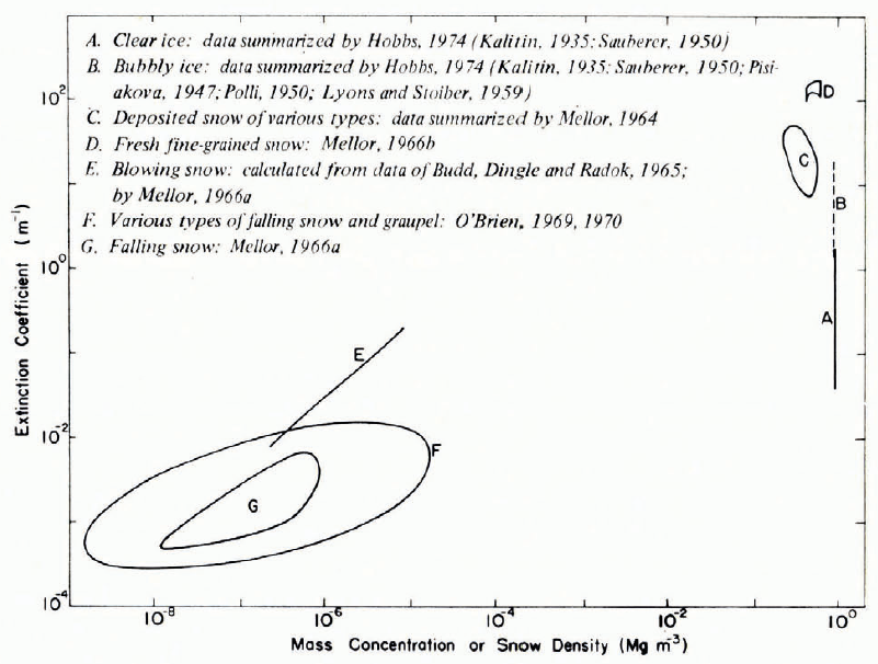
Fig. 29. Extinction coefficient plotted against density for a wide range of snow types. A 1:1 slope on this log–log plot would imply direct proportionality.
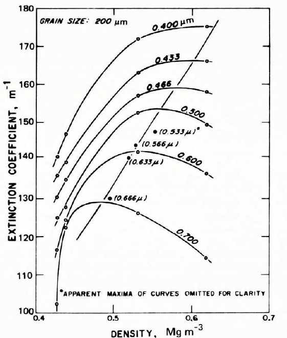
Fig. 30. Extinction coefficient as a function of density for fine-grained snow. The parameter is wavelength. (Reference MellorMellor, 1966[b].)
Grain size is clearly important in determining v. If a large block of clear ice is broken into fragments of fairly uniform size, the transparency of a layer of given thickness obviously decreases as the fragment size decreases, even though the porosity (or density) remains constant (at about 40% porosity for fragments shaken down under gravity). A 100 mm layer of cocktail-size ice cubes is much more transparent than a 100 mm powder layer of too p.m ice grains. Figure 31 gives some data for the variation of measured extinction coefficient with grain size in dry snow of approximately constant density; v decreases with grain size, which is qualitatively in agreement with the theoretical prediction of Reference Bohren and BarkstromBohren and Barkstrom (1974).
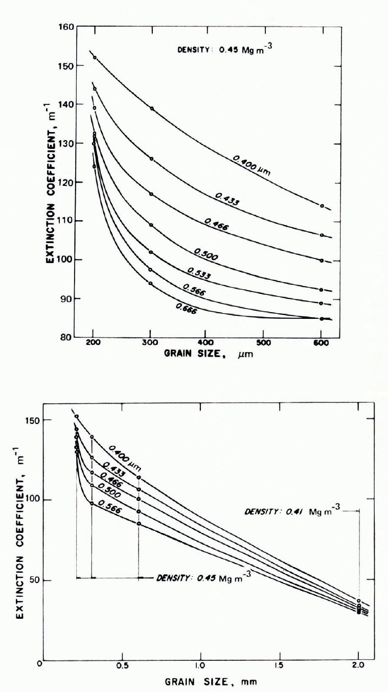
Fig. 31. Extinction coefficient as a function of grain size, with wavelength as parameter. (Reference MellorMellor, 1966 [b].)
Available data for variation of v with wavelength λ do not show a consistent trend for all snow types. Reference MellorMellor (1966[b]) found little spectral selection in the wavelength range 0.4 ˂ λ ˂0.7 μm for coarse-grained dense snow, both wet and dry, but in fine-grained dry snow, v decreased with increase of λ (Fig. 32). By contrast, Reference LiljequistLiljequist (1956) and Reference ThomasThomas (1963) measured an increase of v with increasing λ (Fig. 33). Reference Bohren and BarkstromBohren and Barkstrom (1974) point out inadequacies in various measuring techniques, and calculate a trend that is in good agreement with the Liljequist data, i.e. v increasing with λ.

Fig. 32. Extinction coefficient as a function of wavelength for a range of snow types. (Reference MellorMellor, 1966[b].)
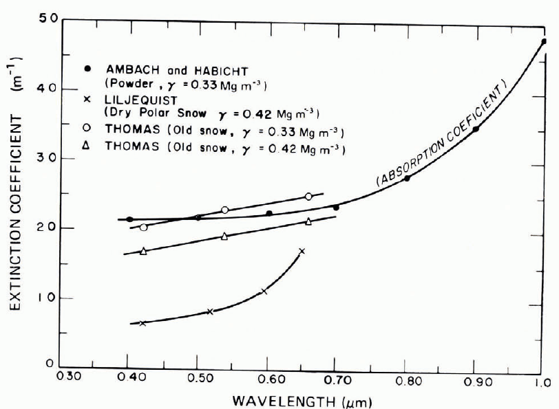
Fig. 33. Extinction coefficient as a function of wavelength according to various investigators.
Spectral reflectance
The reflectance of snow is determined by the illumination conditions, by the characteristics of the surface, and by sub-surface backscattering. With diffuse illumination (e.g. overcast sky) and with a smooth snow, a Lambert surface can be assumed (reflected intensity proportional to cosine of reflection angle), and a simple value of reflectance defined. With directional incident radiation (e.g. direct sunlight), the reflectance is also directional, especially if the snow surface has directional roughness characteristics (e.g. sastrugi, dunes, ablation pits). Although reflectance r varies with wavelength λ, there is not much spectral selection in the visible range (snow looks white in “white” light), and a mean reflectance, or albedo, is often used. The albedo A for wavelengths from λ1 to λ2 is

where I and rI are incident and reflected intensities at wavelength λ. λ 1 and λ2 are usually determined by the response characteristics of the measuring device.
Clear ice has a very low extinction coefficient in the visible range, so that a thick layer with a clean flat surface has very low reflectance; for normal incidence of visible light, the reflectance or albedo is about 0.02, or 2%. Bubbles and cracks introduce internal scattering, and reflectance can increase abruptly to values in excess of 0.5. In snow, the grain boundaries have a strong scattering effect, and diffuse reflectance values approach 100% for deep layers of fresh fine-grained material that has angular grains and little intergranular bonding (i.e. snow with high extinction coefficient). For moist or wet snow, the albedo can drop to the 0.6 to 0.8 range.
Albedo obviously decreases with increasing grain size; Reference Bohren and BarkstromBohren and Barkstrom (1974) predict that, like extinction coefficient, albedo will be inversely proportional to the square root of grain size.
For infra-red radiation, the “long-wave albedo” is likely to be appreciably lower than the albedo for the visible range. Reference Bryazgin and KoptevBryazgin and Koptev (1969) give data showing “long-wave” (0.6-1.2 μm) albedo up to 35% lower than the “integrated” albedo (spectral range not given). Their mean values for different snow types are compared in Table II.
Table II. Comparison of “Integrated” and “Long Wave” Albedos
According to Reference Bryazgin and KoptevBryazgin and Koptev (1969)
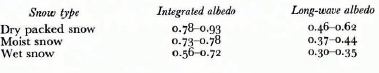
Reference BarkstromBarkstrom (1972) and Reference Barkstrom and QuerfeldBarkstrom and Querfeld (1975) show analytically how albedo for a level surface ought to vary with solar altitude under clear skies, finding fair agreement with field data from Antarctica (Fig. 34). There are, however, Arctic data that fail to show the same effect (Bryazgin and Koptev, 1969).

Fig. 34. Clear-sky albedo plotted against the sine of solar altitude. Lines give theoretical relations according to Reference BarkstromBarkstrom (1972) and Reference Barkstrom and QuerfeldBarkstrom and Querfeld (1975). Triangles and squares give data points from Reference LiljequistLiljequist (1956) and circles give data points from Reference RusinRusin (1961).
Most of the reflection of visible light occurs very close to the surface. Reference TimerevTimerev (1970) found that with fresh dry snow (ρ ≈ 0.31 Mg m-3) and an albedo of 0.90 to 0.94, only about 1% of the reflection was produced by sub-surface returns, although the measuring method that was used seems to leave questions as to how “sub-surface” is defined. In moist snow (ρ = 0.38 to 0.44 Mg m-3) with an albedo of 0.81, some 40% of the reflected intensity came from below the surface. Extrapolating transmission measurements to x = 0 and comparing with reflections from a calibrated Lambert surface, Mellor (1966[b]) found that 20% to 6o% of the reflected intensity from dense dry snow (ρ = 0.37 to 0.62 Mg m-3) could be attributed to sub-surface backscattering (there was also an implication that spectral selection in reflectance occurs in the sub-surface process). Measurements of reflectance as a function of thickness for a finite snow layer Reference Giddings and LaChapelle(Giddings and LaChapelle, 1961) showed that r became effectively independent of thickness above 10 to 20 mm in snow with 0.5 mm grain size (λ = 0.6 μm). Reference Barkstrom and QuerfeldBarkstrom and Querfeld (1975) deduced that the snow thickness required to conceal an underlying layer might be about 5.3 mm, although this value corresponds to an implied extinction coefficient (190 m-1) that seems to be somewhat higher than any measured values.
Some measured values of spectral reflectance r are shown in Figures 35–37. These results are rather inconsistent, perhaps because directional characteristics for direct sunlight differ for different spectral ranges. Another complication is variation of grain size, and possible variation in the relative magnitudes of sub-surface absorption and scattering. Not much variation of r with λ would be expected in the visible range for fine-grained dry snow. Reference Bohren and BarkstromBohren and Barkstrom (1974) predict a weak decrease of r with increasing λ. Figures 36 and 37 show a general decrease of r as snow becomes wet, with the greatest decrease at the red end of the visible range.
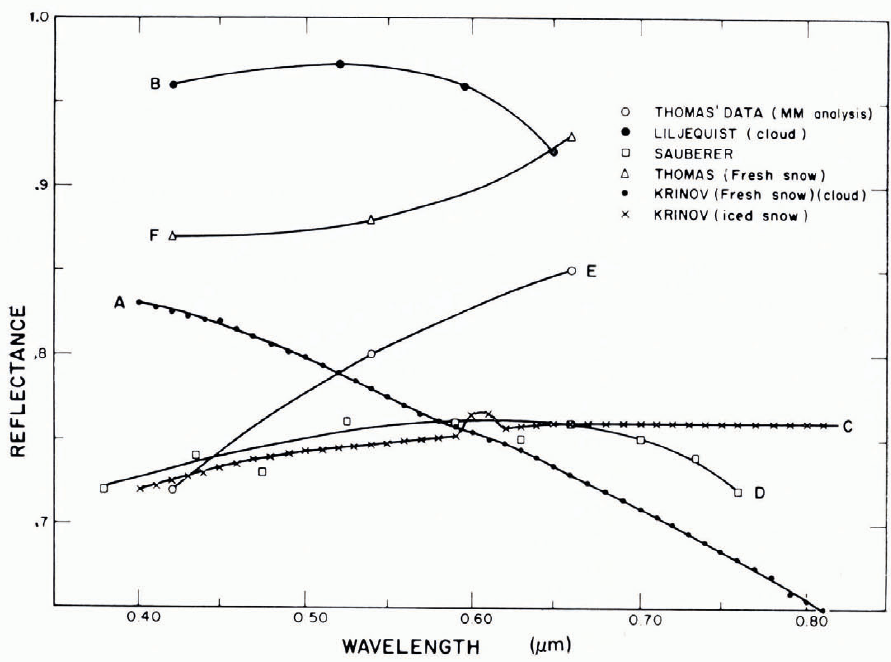
Fig. 35. Reflectance as a function of wavelength according to various investigators.
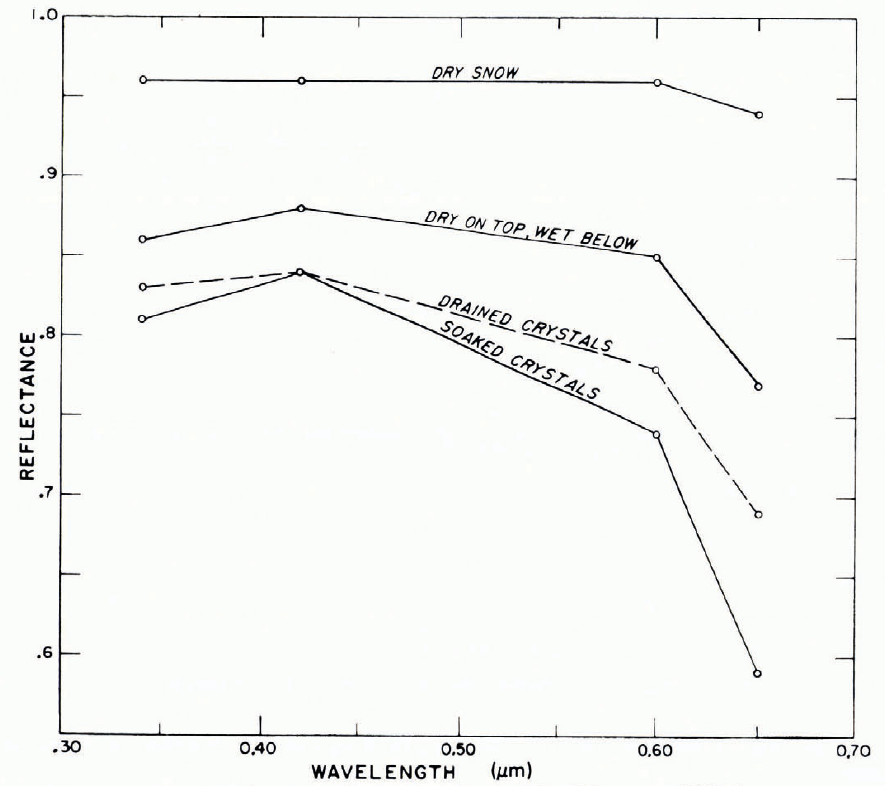
Fig. 36. Reflectance as a function of wavelength. (After Reference HolmgrenHolmgren, unpublished).
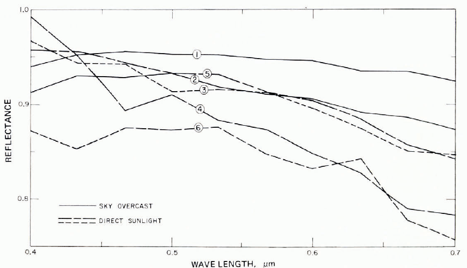
Fig. 37. Reflectance as a function of wavelength. (Reference MellorMellor, 1966[b].)
1. Fresh snow (dry), 0.28 Mg m-3, 0°C.
2. 1-2 cm fresh snow (0.1 Mg m-3) on older snow (0.4 Mg m-3), 0°C.
3. Metamorphosed snow, 0.43 Mg m-3, 0°C.
4. Slightly metamorphosed new snow, 0.2 Mg m-3, 0°C.
5. Wet snow, 2 d old, 0.4 Mg m-3, melting during test.
6. Same as 5 after 5 h mare melting.
Reference O’Brien and MunisO’Brien and Munis (unpublished) measured spectral reflectance through the visible range (0.4 to 0.8 μm) for fresh snow of low density (ρ = 0.14 Mg m-3), finding high reflectance (r > 0.9) with virtually no spectral selection. By contrast, measurements by Reference VickersVickers (unpublished), under varying sky and snow conditions, showed consistent decrease of r with increase of λ between 0.4 and 0.8 μm.
Reference O’Brien and MunisO’Brien and Munis (1975) made detailed measurements of spectral reflectance from the red end of the visible spectrum through the near infrared (0.6 to 2.5 μm), and found high reflectance in the visible, sharp fall-off between 0.7 and 1.5 μm, and very low reflectance above 1.45 μm (Fig. 38). At about 1.8 and 2.25 μm there were local peaks of reflectance that were most pronounced for fresh snow and fine-grained snow. Local peaks in the reflectance curve apparently corresponded to the absorption spectrum of ice. Throughout the range, reflectance decreased with increase of density and increase of grain size, and probably also with decrease of grain angularity and increase of grain bonding. Thawing the snow to a wet state reduced reflectance throughout the range, and refreezing did little to restore higher values. At about 2 μm, the reflectance of thawed snow and refrozen snow was anomalously high in relation to fresh snow. Reflectance varied to some extent with angles of incidence and reflection (with normally incident radiation, reflectance tended to increase as the detector axis moved away from the normal direction).
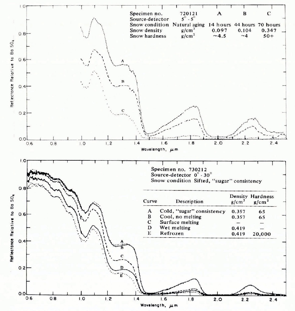
Fig. 38. Relative reflectance as a function of wavelength from the visible through the near infrared, showing effects of snow type and temperature. (From Reference O’Brien and MunisO’Brien and Munis, 1975.)
Reference ZanderZander (1966, Reference Zander1968) made infrared reflectance measurements on ice clouds and hoar frost (Fig. 39). In contrast to the O’Brien and Munis results for snow deposits, reflectance for this very fine-grained material (≈ 2 μm) remained quite high up to about λ = 2.6 μm. The reflectance peaks around 1.8 and 2.25 μm reached as high as 0.8 and 0.55 respectively in ice clouds, whereas the corresponding peaks for snow were never higher than about 0.3 and 0.2 respectively in freshly fallen snow of “low” (0.17 Mg m-3) density. (They were an order of magnitude smaller still in dense old snow that had undergone thawing.)

Fig. 39. Infrared reflectance of ice clouds and hoar frost. (After Reference ZanderZander, 1966.)
Reference VickersVickers (unpublished) measured spectral reflectance from 0.3 to 1.45 μm on progressively decaying snow for various sky conditions (Fig. 40), and found that reflectance remained quite high throughout the range. In the near infrared there was a local peak at about 1.15 μm, and a local minimum near 1.3 μm, but almost all the measurements were above 50% reflectance.

Fig. 40. Reflectance in the visible and near infrared for various conditions. (Reference VickersVickers, unpublished.)
1. Clear sky, air temperature -5°C.
2. Clear sky, air temperature -8°C.
3. Clear sky, air temperature -6°C.
4. 2/10 cloud, air temperature -6°C.
5. 2/10 cloud, air temperature -5°C.
6. Clear sky, air temperature 0°C.
7. Complete cloud cover, air temperature +2°C.
8. Complete cloud cover, air temperature +2°C.
9. Complete cloud cover, air temperature +5°C.
Emissivity
The long-wave emissivity of solid ice is high, values around 0.97 generally being accepted. Early observations on wet snow gave values of emissivity that were very close to unity, but measurements by Dunkle and others (Reference Dunkle and GierDunkle and Gier, 1955; Reference DunkleDunkle and others, 1957) indicated that emissivity, or emittance, decreased with decreasing grain size and with decreasing temperature (Fig. 41); values as low as 0.82 were measured. The physical reasons for these variations do not seem to have been explored, although there are hints that surface properties of the grains and the porous mass may hold the key to emissivity variations. New emissivity measurements will soon be made by CRREL.

Fig. 41. Long-wave emissivity as a function of temperature. (Reference Dunkle and GierDunkle and Gier, 1955; Reference DunkleDunkle and others, 1957.
Conclusion
Snow is clearly a very complicated material, especially at temperatures near the melting point. It is also a highly variable material, with some properties that change by several orders of magnitude as bulk density varies over the typical range of deposited snow. Nevertheless, the general properties of snow are fairly well understood, and the main problem for practicing engineers is in locating the relevant data, which tend to be scattered through relatively inaccessible reports and publications. Where more detailed understanding of the material is called for in the R &D area, there are still some major inadequacies. For example, snow mechanics still remains a somewhat confused field, optical characteristics could perhaps be better defined, and the properties of wet snow need more systematic attention.
Snow is a very abundant material, its impact on human affairs is steadily increasing, and consequently increasing demand for technical information might be expected. It has been estimated that the direct cost of snow on roads and airfields in the U.S. alone is about half a billion dollars annually, and the U.S. Environmental Protection Agency has recently estimated total annual cost as almost 3 billion dollars, but the relevant technology appears almost stagnant. Industrial activity in severe snow environments has been increased by resource developments in the Arctic, and by developments in mountain regions. Satellite technology offers revolutionary possibilities for monitoring snow cover over vast areas, with immediate potential benefits in snow hydrology, provided that the unspectacular but essential research on optical and dielectric properties gets done. Higher energy costs have increased some potential benefits and penalties associated with snow, while population pressures tend to increase the importance of water resources and the agricultural aspects of snow. In the military field, snow has the potential to play havoc with a wide range of systems and operations, and to introduce unpredictable elements. For example, vehicle mobility (not much improved since World War II) can be troublesome, optical and microwave systems can suffer, fixed installations can be put temporarily out of action, and things such as blast effects and projectile impact phenomena are only roughly predictable (there also remain the kind of problems that plagued N. Bonaparte, A. Hitler, and others). Finally, recreation industries based on snow (skiing, snowmobiling) stand to benefit from improved capabilities in snow engineering.
Expectations of an accelerating demand for technical information on snow are not fully in accord with the apparent facts of the situation. In the twelve years since this writer last made a general review of the engineering properties of snow, available data have increased, but hardly at a more rapid pace than in the decade preceding 1964. There are plenty of responsible institutes, agencies, committees, societies and commissions, and R &D expenditures are still running at high levels (one large institute has more than doubled its budget over the past twelve years); nevertheless, there is not much evidence of large-scale systematic research in the field. This may be due partly to the existence of an information gap between the research community and potential users of technical information. For example, of the thousands of municipal engineers who deal with snow at great expense every year, there can be few who have much technical knowledge of the material they are handling; there is effectively no access to suitable books or technical training, and therefore no foundation for a professional approach.
There seems a good possibility that increased efforts in information transfer and applied research on snow could yield substantial economic benefits, a situation which ought to interest research managers and policy makers.
Discussion
A. DYUNIN: Do you know a bout investigations on the combined influence of a ll five physical field s on the snow behavior (kinematics of wind, electrical charges of air and snow flakes, thermal conditions, gravitation, static pressure)?
NI. MELLOR: I thought at first that the question was concerned with potential fields, but it seems to refer to the combined effects of several factors on the behavior of snow suspended in air. In determining properties of materials, we usually try to separate the effects of the independent variables, but perhaps the concern here is with the motion of wind-blown particles under the influence of the factors named in the question. I do not know of studies that consider systematically the combined effects of these factors, but I agree that they are all significant.
D. V. REDDV : Would not hydrodynamic theory be adequate for plastic-wave propagation in low-density snow?
MELLOR: I believe that hydrodynamic theory would be appropriate for dealing with highspeed plastic waves in low-density snow. Hydrodynamic theory, in which shear resistance is of minor importance, is usually applied in considering close-range effects a round an explosion in a compressible solid medium. When snow of very low density strikes an obstacle, as in a dust avalanche, the steady impact stress is probably given adequately by the stagnation pressure for a fluid of equivalent density. The rise time for initial impact may be drawn out by the precursor wave, perhaps reducing the initial peak stress.
J. L. DAVIS: You have divided the electromagnetic spectrum into electrical and optical wavelengths. Have you found any relevant work in the gamma-ray wavelengths of the spectrum ?
MELLOR: I have not come across any systematic studies for gammaradiation, but gamma density probes have been used experimentally in snow for many years. Gamma-ray systems have also been used for measuring the amount of snow cover, or water-equivalent of the snowpack.
J. MARTINEC (written comment): The absorption coefficient p- in the equation Ix = I0 exp (- (μx) where I0 is the initial radiation, Ix is the attenuation radiation, μ is the absorption coefficient, and x is the water-equivalent of snow, depends on the hardness of the gamma radiation. For 60Co gamma rays (1.l - 1.3 MeV) it was determined as μ = 0.063 cm- I.
L. LLIBOUTRY: Which parameters seem to you the best ones to define conveniently one kind of snow? For a long time engineers gave only the density. We must also keep in mind that often snow has been modified by human activity, skiers for instance.
MELLOR: Density is a good description, because many properties are strongly dependent on density or porosity. Some change by orders of magnitude as density varies over the common range. Density is also easy to measure. Intergranular bonding is also important. I can think off-hand of properties that change in magnitude by a factor of three as dry snow changes from the unbonded state to fully sintered condition without change of density. Grain size of dry snow tends to stay within a rather narrow range after deposition and initial metamorphism, except for depth hoar. Dry snow modified by skiers may not differ very much from natural snow of the same density. Temperature is obviously important, so is liquid-w.,ter content in wet snow and perhaps we shall soon have better ways to describe it.


