


1. Introduction
The jet in crossflow (JICF) is a canonical flowfield that also has significant practical importance due to its ease of implementation and excellent mixing characteristics (Karagozian Reference Karagozian2010). The JICF exhibits several distinct vortical structures (New, Lim & Luo Reference New, Lim and Luo2006), of which the shear layer vortices (SLV) are a dominant component of the near field and the focus of this study. A reacting JICF (RJICF) has a number of additional degrees of freedom relative to a non-reacting JICF, including gas expansion ratio due to combustion, transverse location of the flame with respect to the shear layer, streamwise location of the flame (e.g. amount of flame lifting), and flame lifting asymmetry on the leeward and windward sides of the jet (Nair et al. Reference Nair, Sirignano, Emerson and Lieuwen2022). This work expands upon the Nair et al. (Reference Nair, Sirignano, Emerson and Lieuwen2022) analysis of SLV dynamics in an RJICF by exploring its stability characteristics and developing scaling models to capture SLV behaviour across a range of combusting flow conditions.
SLV are formed primarily by concentration of vorticity in the jet shear layers, due to the Kelvin–Helmholtz instability. One of the earliest attempts at characterizing their frequencies was presented by Fric & Roshko (Reference Fric and Roshko1994). From the spatial positioning of these structures, a characteristic length and jet velocity ( $u_{{j}}$) scale was used to define the SLV frequency via the Strouhal number $St = f d_{{j}}/u_{{j}}$, where $d_{{j}}$ and $u_{{j}}$ denote the jet diameter and velocity, respectively. However, subsequent work has demonstrated clearly that such a frequency scaling is incomplete. For example, Megerian et al. (Reference Megerian, Davitian, de B. Alves and Karagozian2007) notes that the characteristic frequencies ( $St$) defined in this way are not constant, but depend on the jet exit velocity profile. Sharper, top-hat profiles produce high-frequency structures in the range $St \sim 0.75\unicode{x2013}2.0$ (Fric & Roshko Reference Fric and Roshko1994; Smith & Mungal Reference Smith and Mungal1998), while parabolic profiles (fully developed pipe flow) have lower values, ${St} \sim 0.3$ (Camussi, Guj & Stella Reference Camussi, Guj and Stella2002). The momentum thickness ( $\theta$), which quantifies the shape of the velocity profile, is more likely the appropriate characteristic length scale for these instabilities, as might be expected. To this effect, spectral data taken by Megerian et al. (Reference Megerian, Davitian, de B. Alves and Karagozian2007) along the windward shear layer demonstrated that the scaling $St_{\theta } = f\theta / u_{{j}}$ did reduce variability in observed frequencies at different local jet Reynolds numbers $2000 < Re_{{j}} < 3000$ and exit velocity profiles (i.e. different $\theta$ values). But these same data also demonstrated that $St_{\theta }$ was also a function of $J$, the jet to crossflow momentum flux ratio ( $\rho _j u_j^2/\rho _{\infty } u_{\infty }^2$), and, in a follow-on study focusing on density stratified JICF (Getsinger, Hendrickson & Karagozian Reference Getsinger, Hendrickson and Karagozian2012), it was also shown to depend on $S$, the jet to crossflow density ratio ( $\rho _j/\rho _{\infty }$). This illustrates that additional parameters influence SLV frequencies.
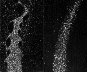
Consider next the spatial evolution of the shear layer spectral content. Studies (Megerian et al. Reference Megerian, Davitian, de B. Alves and Karagozian2007; Getsinger et al. Reference Getsinger, Hendrickson and Karagozian2012) have noted a strong narrowband spectrum (figure 1b), relatively constant in the streamwise direction, for cases with  $J < 10$ and $S < 0.45$, suggestive of globally unstable behaviour (Huerre & Monkewitz Reference Huerre and Monkewitz1990). At higher $J/S$ values, the spectrum was broader, peaking in the near field, transitioning to a dominant subharmonic mode farther downstream (figure 1a), consistent with convectively unstable behaviour. This instability behaviour has strong influences on jet dynamics (Megerian et al. Reference Megerian, Davitian, de B. Alves and Karagozian2007; Getsinger et al. Reference Getsinger, Hendrickson and Karagozian2012) and responsivity to external forcing (Narayanan, Barooah & Cohen Reference Narayanan, Barooah and Cohen2003). These convective/global instability trends have similarities to free jets, which are self-excited either when an external counter-current is applied (Strykowski & Niccum Reference Strykowski and Niccum1991) or in cases where the density of the jet is sufficiently low (Monkewitz & Sohn Reference Monkewitz and Sohn1988). Noting this, Iyer & Mahesh (Reference Iyer and Mahesh2016) pointed out that the stagnation point created by the crossflow in JICF leads to a region of counterflow upstream of a JICF – effectively setting up a counter-current shear layer (CCSL), and providing a mechanism for the transition to global instability even at iso-density JICF conditions. This counter-current velocity $U_2$ and jet velocity ( $U_1 = u_{{j}}$) can be used to define the counter-current velocity ratio $\varLambda = (U_1-U_2)/(U_1+U_2)$, which, along with the density ratio across the mixing interface $S = \rho _1/\rho _2$, has been shown to parametrize the transition to absolute instability in a two-dimensional parallel stability framework for wakes and jets (Huerre & Monkewitz Reference Huerre and Monkewitz1985). Since global instability is a special case of the shear layer exhibiting absolute instability over a large spatial region (Huerre & Monkewitz Reference Huerre and Monkewitz1990), the extracted $\varLambda$ values from iso-density (Iyer & Mahesh Reference Iyer and Mahesh2016) and stratified JICF (Shoji et al. Reference Shoji, Harris, Besnard, Schein and Karagozian2020) experiments have been compared with theoretical values, obtained from the parallel flow framework for axisymmetric counter-current jets (Jendoubi & Strykowski Reference Jendoubi and Strykowski1994), corresponding to the transition to absolute instability. These theoretical contours ( $S_{{crit}}$, $\varLambda _{{crit}}$) agree well with the observations from experiments and provide a viable model, despite the three-dimensionality of the flowfield, to explain the observed dependence of global/convective instability boundaries on $S$ and $J$.
$J$.

Figure 1. Transverse velocity spectra (in dB) sampled from the windward shear layer of a flush jet for different velocity ratios (R) showing (a) convectively (amplifier) and (b) globally unstable behaviour (Megerian et al. (Reference Megerian, Davitian, de B. Alves and Karagozian2007)). (c) Stability boundaries from previous non-reacting studies (Megerian et al. Reference Megerian, Davitian, de B. Alves and Karagozian2007; Getsinger et al. Reference Getsinger, Hendrickson and Karagozian2012): red indicates globally unstable, blue indicates convectively unstable; marked points correspond to parameters explored in this study and elaborated in § 2.1.
As demonstrated in Nair et al. (Reference Nair, Sirignano, Emerson and Lieuwen2022), reacting configurations provide additional degrees of freedom (i.e. exothermicity, stabilization location) that influence the transitional contour observed for non-reacting cases (figure 1c). Specifically for the case of an RJICF, Sayadi & Schmid (Reference Sayadi and Schmid2021) demonstrated that a reacting jet shows lower characteristic frequencies compared to non-reacting jets across the same parameters ( $J$ and $S$), and also stronger responsivity to external forcing – hypothesized to be connected to a flame instability.
In an attempt to capture dominant physics, researchers have often reduced these problems to simpler, canonical shear flows where the effect of combustion is modelled by considering the impact of heat release on parallel base flow, i.e. through an imposed density stratification (Shin & Ferziger Reference Shin and Ferziger1991). Mahalingam, Cantwell & Ferziger (Reference Mahalingam, Cantwell and Ferziger1991) demonstrated, using a parallel flow framework, that for an axisymmetric co-flowing jet, the effect of combustion was captured primarily by modelling the flame as an imposed base flow density stratification, and that the contribution of the linearized heat release fluctuations was negligible. The experiments performed by Clemens & Paul (Reference Clemens and Paul1995) compared growth rates between a reacting jet and a non-reacting jet with a density stratification (modelled with respect to the flame-induced density stratification), showing that the observations were consistent with the above hypothesis; i.e. that the reaction zone appears to act primarily as a density boundary condition at the mixing interface. These arguments provide credence to the idea that the stability behaviour of certain RJICF configurations can be captured potentially by simply considering the flame-induced density stratification as an additional parameter.
Some insight into why density stratification influences stability behaviour in shear layers can be gained from a generalization of Rayleigh's inflection point theorem (Drazin & Reid Reference Drazin and Reid2004) – namely, that a necessary condition for temporal instability in a parallel flow is the presence of an inflection point in the density-weighted vorticity,  $\rho _0\omega _0$ (Coats Reference Coats1996), where $\rho _0$ is the base flow density, $U_0$ is the base flow velocity, $y$ is the spanwise coordinate, and $\omega _0 = {\rm d}U_0 /{{\rm d} y}$ is the vorticity. When density variations are introduced through flames or simply non-uniform gas properties, the magnitude and nature of the density-weighted inflection in $\rho _0\omega _0$ can change. Thus the existence of multiple extrema in the $\rho _0\omega _0$ profile suggests the presence of multiple modes with different stability behaviours (Jackson & Grosch Reference Jackson and Grosch1990), i.e. absolutely versus convectively unstable modes. For example, in the special case of buoyant reacting jets, Juniper, Li & Nichols (Reference Juniper, Li and Nichols2009) noted that the transition to absolute instability is influenced by the inflection point (for the $\rho _0\omega _0$ profile) that lies outside the flame surface, while the inner inflection point is stabilized due to the flame-induced stratification.
The position and characteristics of these points of inflection can also be modified by changing the radial flame stabilization location (i.e. the flame shear layer offset). Emerson & Lieuwen (Reference Emerson and Lieuwen2015) modelled a premixed flame in a bluff-body wake flowfield, noting that as this offset from the shear centre was increased in either direction, the transitional value (with respect to the wake velocity ratio of the flame) to absolute instability changed, and in the limit of large offsets, the solution reverted to the iso-density value. In the case of a single mixing layer with a diffusion flame-like stratification, this effect is not symmetric. Hajesfandiari & Forliti (Reference Hajesfandiari and Forliti2014) noted a significantly increased instability growth rate when the flame was moved towards the high-velocity stream, analogous to the flame being moved ‘inside’ the shear layer in a jet diffusion flame. But experimental evidence from Füri et al. (Reference Füri, Papas, Raïs and Monkewitz2002) performed on co-flowing jets, and even the results presented in Nair et al. (Reference Nair, Sirignano, Emerson and Lieuwen2022), demonstrate clearly additional effects in play – in fact, these studies observed the opposite behaviour. For the case where the flame was moved inside the shear layer, increased local viscosity likely contributes to the stabilization of the jet shear layer. This indicates that additional combustion effects – i.e. strong influences on local viscosities/Reynolds numbers – also have strong influences on the problem. Indeed, recent non-reacting JICF stability studies have demonstrated that small changes ( $\sim$10 %) in the jet absolute viscosity ( $u_{{j}}$) can change the value of $J_{{crit}}$, at which the jet transitions to global instability (Shoji et al. Reference Shoji, Harris, Besnard, Schein and Karagozian2020). Previously, studies (Shan & Dimotakis Reference Shan and Dimotakis2006; Megerian et al. Reference Megerian, Davitian, de B. Alves and Karagozian2007) have noted that JICF dynamics (trajectory, frequency scaling) are relatively insensitive to Reynolds numbers for $Re_j > 2000$, while below $Re_j < 600$, changes to the jet topology, due to the stabilization of the shear layers, were observed (Blanchard, Brunet & Merlen Reference Blanchard, Brunet and Merlen1999; Camussi et al. Reference Camussi, Guj and Stella2002). Given that the fluid viscosity can increase by almost an order of magnitude due to combustion, it is very plausible for combusting experiments to fall inside this $Re_j$-dependent regime, even while the non-reacting cases at identical $J$ and $S$ values are $Re_j$-independent. Indeed, for atmospheric pressure configurations, most RJICF experiments with attached flames will fall in this $Re_j$ regime (Nair et al. Reference Nair, Sirignano, Emerson and Lieuwen2022), just by virtue of the need to keep the flame from blowing off. As such, additional Reynolds number effects, in addition to inviscid, inertial effects, can lead to differences in RJICF and JICF dynamics – as we show in this study, this occurs for cases where the flame lies inside the shear layer.
This work seeks to clarify further how combustion influences RJICF behaviour, with a particular focus upon three parameters –  $J$,
$J$,  $S$ and the radial flame position. The test matrix design philosophy is similar to that in Nair et al. (Reference Nair, Sirignano, Emerson and Lieuwen2022), but with focus on high-frequency/spatial resolution diagnostics (40 kHz stereo particle image velocimetry, SPIV), needed to resolve SLV frequencies and spatial development.
2. Diagnostic details and data processing methodology
2.1. Test matrix and diagnostic set-up
This section summarizes key details of the test matrix, and the set-up for the high-speed SPIV experiments; more exhaustive details on the facility and test matrix, including baseline data for the crossflow and experimental design decisions, can be found in Nair et al. (Reference Nair, Sirignano, Emerson and Lieuwen2022). Three flame-flow configurations were considered – non-reacting (NR), reacting where the flame lies outside the shear layer (R1), and a reacting case where the flame lies inside (R2). The jet composition was controlled to obtain the different  $S$ values as well as flame configurations, and is summarized in table 1. The jet mass flow rate was varied to study three $J$ values, namely 6, 12 and 18 (table 2). The $J = 30$ cases (Nair et al. Reference Nair, Sirignano, Emerson and Lieuwen2022) were not evaluated (marked with * in table 2) due to limitations with the diagnostic system, but the case numbers corresponding to these cases were retained for consistency with the previous study (Nair et al. Reference Nair, Sirignano, Emerson and Lieuwen2022). The uncertainties in estimating the primary jet parameters presented in table 2 ( $J$,
$J$,  $S$ and $Re_{{j}}$) are estimated to be 9 %, 3 % and 4 %, respectively. These values were obtained using standard error propagation techniques using the measurement error of the mass flow and temperature measurement systems for the jet and crossflow.
Table 1. Target jet composition for different configurations.

Table 2. Measured test conditions for 40 kHz  ${\rm SPIV}$.

This combination of  $S$ and $J$ values was chosen to correspond to values that would correspond to being both convectively and globally unstable for non-iso-density, but non-reacting JICF, following Getsinger et al. (Reference Getsinger, Hendrickson and Karagozian2012) (figure 1c). In the R2 configuration, the flame was lifted at the $J = 18$ case, so we present data only for $J=6$ and 12. The value of $S$, as denoted in the stability map, is defined based on non-reacting jet and crossflow values, noting, of course, that there is an additional density ratio in the problem, associated with flame-induced density variation. We will develop an approach that parametrizes this additional density ratio in § 3.3.
The use of high-speed CMOS cameras introduces an inherent trade-off in data acquisition rates and number of acquired pixels. We designed the imaging system with the following two constraints in mind: (1) temporally capturing the dominant spectral peaks without spectral aliasing; (2) sufficient spatial resolution to capture the shear layer structures, which led to imaging resolution  ${\sim }110\ {\rm pixels}\ {\rm mm}^{-1}$. Consequently, this study utilized a much faster sampling rate (40 kHz) and a smaller interrogation region than used in Nair et al. (Reference Nair, Sirignano, Emerson and Lieuwen2022), spatially spanning $2.8d_{{j}} \times 3.3d_{{j}}$ in the plane of symmetry in the near field of the jet (figure 2). Illumination was provided via a pulsed Nd:YAG laser (Continuum Mesa particle image velocimetry, PIV) operating at 40 kHz with pulse width 150 ns. Two Photron SA-Z CMOS cameras, fitted with Tamron ( $\,f/\#=8.0$) 180 mm macro lenses, were used to capture the Mie scattering images while arranged in a side scatter configuration at an angle of $25^{\circ }$ each. A Semrock brightline bandpass filter ( $532 \pm 10\ {\rm nm}$) was used to limit the exposure to only scattered light. The PIV pulse spacing was varied between 3.5 and $12\ \mathrm {\mu } {\rm s}$ to ensure an optimal pixel displacement between 12 and 16 pixels, considering the jet velocity scale within the core of the jet in each case. The seed used was commercially available rutile TiO $_2$ with particle mean diameter between 200 and 300 nm. Assessing the Stokes number provides a conservative cut-off frequency estimate 90 kHz (Mei Reference Mei1996), more than twice the sampling frequency, therefore demonstrating that the particles can follow the flow even in the event of moderate clumping and aggregation. Approximately 14 000 samples were acquired, spanning a sampling duration ${\sim }0.4\ {\rm s}$, significantly longer than the time scales of interest in the flowfield.

Figure 2. (a) Diagnostic set-up with field of view in the near field. Instantaneous data showing (b) raw Mie scattering images for case 6, and (c) normalized out-of-plane vorticity with streamlines calculated from the in-plane velocity components ( $u,v$).
The raw Mie scattering data (figure 2b) were processed to obtain the vector fields using LaVision Davis 8.3.1 software. Multi-pass vector processing was performed using a square interrogation window of size  $48 \times 48\ \mathrm {pixel}^2$ for two passes initially, and two final interrogation passes using a $12 \times 12\ \mathrm {pixel}^2$ Gaussian window, to get sufficiently good correlation values. For the R2 cases, due to a lower seed density, a final window size $16 \times 16\ \mathrm {pixel}^2$ was used to obtain sufficiently high correlation values. The universal outlier detection scheme was used to remove outlier vectors and interpolate gaps, finally smoothing with a $3 \times 3\ \mathrm {pt}^2$ Gaussian filter. The final interrogation window size used to obtain vectors was approximately $150\ \mathrm {\mu } {\rm m}$ with 50 % overlap between adjacent windows.
2.2. Vortex tracking
The vortex identification technique discussed in Nair et al. (Reference Nair, Sirignano, Emerson and Lieuwen2022) is utilized to identify shear layer vortices in the jet near field. This technique employs topological segmentation (Bremer et al. Reference Bremer, Gruber, Bennett, Gyulassy, Kolla, Chen and Grout2015) of the swirling strength criterion ( $\lambda _{{ci}}$) (Zhou et al. Reference Zhou, Adrian, Balachandar and Kendall1999), which captures regions of rotation from the velocity gradient field. These vortices for an instantaneous snapshot of the velocity field are marked using solid black lines in figure 3(a).

Figure 3. (a) Detected vortex field for an instantaneous snapshot  $F(t)$ and predicted subsequent field $F'(t)$. (b) Detected vortex field for an instantaneous snapshot at the subsequent time step $F(t+\delta t)$ (solid line) with the predicted field $F'(t)$ (dashed line).
The current study extends further the vortex identification process to track vortices across successive snapshots of the flowfield, given the higher sampling frequency of the data. Using the instantaneous vortices at a time instant  $F(t)$ (figure 3a), a guess for the future orientation of these vortices is obtained using the mean velocity field $(\bar {u},\bar {v})$ to obtain the guess field $F'(t)$. Now this field, $F'(t)$, is compared with the obtained vortex detection field for the subsequent time step $F(t+\Delta t)$, and the structures correlated based on the overlap of their predicted positions (figure 3b). Essentially, this allows for the identification and tracking of a vortex $i$ in space and time as it advects through the measurement region of interest.
The information on vortex centroid positions can be compiled into  $s\unicode{x2013}t$ plots as shown in figure 4(b), capturing the space–time dynamics of the windward SLV. These plots allow for the characteristic length scales – i.e. the spacing between the vortices – and the characteristic time scales to be extracted by ensemble averaging the vertical and horizontal spacing between each vortex track. The dominant Strouhal number will thus correspond to the most probable time scale of vortex passing, which can be sampled at any streamwise location (figure 4c). Similar plots have been used by both Hernan & Jimenez (Reference Hernan and Jimenez1982) and D'Ovidio & Coats (Reference D'Ovidio and Coats2013) to extract characteristic frequencies as well as study the role of vortex pairing in the growth of planar mixing layers.

Figure 4. (a) Instantaneous vorticity snapshot for case 6:  $J = 12$, $S = 1.0$, NR showing detected boundaries of vortical structures (solid line) and characteristic vortex centroid spacing ( $\lambda$) between the vortex centroids (*). (b) Plots of $s$ versus $t$ vortex time histories. (c) Histogram of characteristic time scale ( $\tau$) of vortex passing as sampled at $s /d_j = 3$.
2.3. Shear layer spectrum extraction
This subsection describes the method for extracting the spatial evolution of the velocity spectrum, and extraction of the dominant characteristic natural frequencies ( $St$). Previous studies focusing on characterizing the behaviour of non-reacting jets utilized hot-wire anemometry in the near-field shear layer (Megerian et al. Reference Megerian, Davitian, de B. Alves and Karagozian2007; Getsinger et al. Reference Getsinger, Hendrickson and Karagozian2012). In addition to quantifying the spectra and obtaining the characteristic non-dimensional Strouhal numbers, $St= fd_j/u_j$, they also tracked the spatial spectral evolution along the jet-oriented streamwise coordinate ( $s$), and consequently demonstrated clear variations in the spectral behaviour of globally unstable and convectively unstable shear layers. A similar approach is employed in this study, where velocity data, obtained from SPIV, are extracted from the shear layer and are used to quantify the spectral behaviour and characteristics. Due to the orientation of the shear layer along the plane of symmetry, and considering the dominant direction of vorticity, $\omega _z$, the unsteady streamwise velocity (with respect to the crossflow) $u'$ and the transverse velocity $v'$ both show strong spectral content corresponding to the SLV structures while $w'$ will likely be significantly weaker. Here, the transverse velocity spectrum $v'$ is chosen, as the choice of reference velocity scale ( $u_j$) is straightforward since the measurements are made in the shear layer and $v'\sim u_j$.
In RJICF configurations, jet flapping can alter the jet trajectory on a periodic basis due to fluctuations in the crossflow, originating from combustion-driven axial acoustic oscillations from the vitiator (Wilde Reference Wilde2014). While the jet flapping can alter the trajectory on an instantaneous basis, the time period associated with flapping is much longer than that associated with the shear layer instabilities, and the jet trajectory can be considered quasi-stationary. For the current configuration, axial velocity data from the crossflow (Nair Reference Nair2020) show energetic modes around 80 Hz. Proper orthogonal decomposition was also performed to further correlate this 80 Hz mode, with the orthogonal modes associated with jet flapping in a JICF (Meyer, Pedersen & Özcan Reference Meyer, Pedersen and Özcan2007). Despite the quasi-stationary nature of the jet flapping, the approximate trajectory of the jet does vary over the total measurement time period ( $\sim$0.4 s), therefore the probe locations for the transverse velocity spectrum need to be conditioned with the jet trajectory.
This is also necessary for reacting cases (R1) where jet flapping would result in probe points fixed in the laboratory frame of reference ( $x\unicode{x2013}y$) to sample velocity data from inside the flame intermittently, despite the flame lying outside the shear layer. The instantaneous data in the Cartesian coordinate system ( $x\unicode{x2013}y$) (figure 5a) are converted to a jet-oriented trajectory system ( $s\unicode{x2013}n$) (figure 5b). As the instantaneous vector fields do not have a well-defined potential core, and consequently the centre streamline is not guaranteed to follow the ‘mean’ jet trajectory, a pseudo-instantaneous jet trajectory is computed from the mean velocity field taken from seven sequential vector fields centred around each instantaneous snapshot (figure 5b). Due to the high time resolution of the vector data, the time period across which this average is computed ( ${\sim }175\ \mathrm {\mu } {\rm s}$) is still significantly lower than the time period of jet flapping ( ${\sim }12.5\ {\rm ms}$), and therefore would still be effective in conditioning the instantaneous data with respect to the jet trajectory.

Figure 5. (a) Instantaneous out-of-plane vorticity normalized with respect to the characteristic jet velocity and length scales with a denoted centre streamline (solid line) and the fit of the approximate instantaneous trajectory (dashed line) for coordinate transformation. (b) Mean vorticity (from the pseudo-instantaneous velocity field) in the  $s\unicode{x2013}n$ coordinate system with sample points on the windward shear layer; points in yellow correspond to points at which the transverse shear layer spectra are sampled and displayed in (c).
The normalized transverse velocity spectrum sampled from three positions along the windward shear layer is plotted in figure 5(c). The spectrum was calculated using Welch's power spectral density estimate using windows of 512 data points (spanning  $\sim$12.8 ms) and 50 % overlap. The spectrum indicates that the dominant amplified frequencies evolve spatially in the shear layer – a feature of convectively shear layers that behave as amplifiers, to be covered in § 3.2. A convenient representation of spatially varying instabilities is to use a contour plot (log scale) as in figure 6(b). Given the high-frequency nature of these instabilities, to ensure that the frequencies detected were not aliased with respect to the sampling frequencies, a similar contour plot can be created using the time scales extracted from the $s\unicode{x2013}t$ plots (§ 2.2), where the plot captures the most probably frequency scale at each spatial location (figure 6a). The plots demonstrate that the variation in the dominant frequencies is a direct consequence of vortex pairing leading to a high-frequency fundamental mode in the near field and a subharmonic mode further downstream.

Figure 6. (a) Probability map showing vortex counts for each  $St$ value at different streamwise coordinates ( $s$). (b) Associated transverse spectrum for the same case 3: $J = 18$, $S = 1.75$, NR.
3. Results
3.1. Shear layer dynamics
This subsection overviews qualitatively the near-field flow structures, focusing on SLV dynamics, before presenting more quantitative analysis later. While comparison of the vortex structure and behaviour between the different cases is detailed in Nair et al. (Reference Nair, Sirignano, Emerson and Lieuwen2022), this subsection focuses on the smaller, higher-resolution field of view. As shown in figure 7, the near-field shear layer rolls up due to the Kelvin–Helmholtz instability, forming concentrated vortical structures that can be identified from the Mie scattering images as regions of flow devoid of seed, due to the strong centrifugal acceleration in the vortex cores (Lecuona, Ruiz-Rivas & Nogueira Reference Lecuona, Ruiz-Rivas and Nogueira2002). As demonstrated in Nair et al. (Reference Nair, Sirignano, Emerson and Lieuwen2022), visually prominent effects of  $J$ and $S$ on vortex strength and growth rate manifest through the level of vortex core seed centrifuging, as well as the vorticity distribution. In addition, due to the inherent asymmetry of the flowfield, the shear layer vortices can be separated into ‘windward’ and ‘leeward’ structures that show distinct behaviours. For high- $Re_j$ jets, the windward shear layers tend to show faster roll-up due to the sharp velocity gradient, and reverse flow region, along the upstream shear layer, while the leeward shear layer is influenced by the recirculation zone in the wake of the jet. This behaviour can be seen while contrasting the vortex roll-up observed for the NR and R1 cases.

Figure 7. Instantaneous snapshots of (a–c) Mie scattering and (d–f) vorticity fields, with centre-plane streamlines indicated in black.
Broadly speaking, non-reacting cases show faster vortex roll-up and consequently, for comparable jet time scales ( $u_j/d_j$), exhibit larger vortex cores and larger local vorticity distributions (figure 7). The strength (or speed) of vortex roll-up can be gauged by noting that the vorticity here can be separated into regions of flow rotation and shear. Consequently, the presence of interconnecting braids of vorticity between structures for the R1 cases suggests that at streamwise locations comparable to the NR case, not all the vorticity has been entrained into these vortices. These observations are consistent with the observation that the shear layer instability growth rate is suppressed in the presence of combustion (Nair et al. Reference Nair, Sirignano, Emerson and Lieuwen2022). Finally, the near field of the (R2) cases shows a dramatically different flowfield, devoid of any vorticity concentration and roll-up. The larger field of view studied in Nair et al. (Reference Nair, Sirignano, Emerson and Lieuwen2022) did show large-scale sinuous jet column undulation farther downstream in this case. The leeward region for this case has been masked out due to the low seed density leading to spurious vectors and low data quality in the wake of the jet.
3.2. Classification of instability behaviour
The shear layer spectra (Megerian et al. Reference Megerian, Davitian, de B. Alves and Karagozian2007) provide an important means of quantifying the instability behaviour as well as identifying whether the shear layer behaves as an amplifier of disturbances (convectively unstable) or exhibits self-excited oscillations (globally unstable). The spectral content is sampled along probe positions in the windward shear layer and is presented as contour plots (figure 6b) of spectral amplitude (dB), where the abscissa contains the Strouhal number calculated with respect to the characteristic jet length and velocity scales,  $St= (fd_j)/u_j$, and the ordinate represents the streamwise location along the jet. To contrast the observed behaviour with NR JICF stability behaviour from previous studies (Megerian et al. Reference Megerian, Davitian, de B. Alves and Karagozian2007; Getsinger et al. Reference Getsinger, Hendrickson and Karagozian2012), on the expected shear layer behaviour, the current study test matrix parameters are mapped onto a stability diagram (figure 1c) based on the critical parameters ( $J_{{crit}}$ and $S_{{crit}}$) for transition to self-excited oscillatory behaviour.
Figure 8 presents the spectral content for the NR cases. From the plots, it is clear that there are common patterns to the contour plots. Cases 1, 2, 3 and 7 all show a fundamental high-frequency tone, dominant in the near field, followed by a dominant subharmonic downstream. This is in line with amplifier-type spectra (Megerian et al. Reference Megerian, Davitian, de B. Alves and Karagozian2007) where a broadband peak of amplified frequencies is observed. These amplified frequencies soon saturate and are replaced by subharmonics as the shear layer thickness grows. As indicated by the Lagrangian vortex tracking data (figure 6a), the subharmonics are generated primarily through vortex pairing, a nonlinear process that is observed in flows without strong natural tones (Strykowski & Niccum Reference Strykowski and Niccum1991). On the other hand, the cases that show the fastest roll-up tend to show a strong, narrowband fundamental mode (cases 9, 10 and 11) that persists through the sampled domain. Globally unstable flows behave as strong self-excited oscillators, thereby demonstrating a high degree of periodicity as well as an absence of vortex pairing (Strykowski & Niccum Reference Strykowski and Niccum1991).

Figure 8. Transverse velocity spectra for the NR cases – plots show spectral amplitude (colour bar) tracking the dominant  $St$ values at different locations along the jet coordinate system ( $s$). The schematic maps the parameters of the explored cases with the instability transitional parameter space with respect to $(J,S)$ $[3, 5]$. Top: instability map with blue indicating amplifier, red indicating self-excited oscillator, and semi-filled (red/blue) indicating intermittent behaviour.
The relative strength between the fundamental and subharmonic also depends on the jet parameters. For some of the cases, a binary classification (amplifier versus self-excited) does not capture that the flow is intermittent, i.e. the system is switching between behaving as a self-excited oscillator and as an amplifier. To better characterize this intermittent behaviour, the time series is analysed with a continuous wavelet transform, using a Morse wavelet. This magnitude spectrogram (figure 9) is calculated from the time series of velocity fluctuations at two locations along the windward jet shear layer close to the jet exit ( $s/d_j = 2.0$) and further downstream ( $s/d_j = 4.0$) for the first 0.06 s of the total time series record. The approximate fundamental (black) and subharmonic frequencies (red) corresponding to the spectral data are marked.

Figure 9. Continuous wavelet transform from the transverse velocity time series sampled at two locations, at points in (a–c) the near field ( $s/d_j = 2.0$) and (d–f) the far field ( $s/d_j = 4.0$) for: (a,d) case 3, $J = 18$, $S = 1.75$; (b,e) case 6, $J = 12$, $S = 1.0$; (c,f) case 9, $J = 6$, $S = 0.35$. Note that the $y$-axis is a logarithmic scale.
Observing this intermittency requires studying simultaneously the time–frequency data as the vortex advects along the jet core, because the process of vortex pairing (subharmonic generation) is itself an intermittent process. Consequently, the locations of any vortex pairs will not be fixed, and the subharmonic and fundamental will not tend to be present at the same spatial location at the same time. For cases that behave as an amplifier (figures 9a,d), this implies that nearer to the jet exit, a majority of the energy content will lie with the high-frequency fundamental, while further away, once a majority of the vortices have paired, the subharmonic has more energy content. When the shear layer is a self-excited oscillator, the spectral content is relatively fixed in the time–frequency domain (figures 9c,f). For some cases (figures 9b,e), while the fundamental stays relatively dominant, there are clear short time periods at the downstream location where the subharmonic is quite strong – suggesting intermittent behaviour where vortex pairing has occurred, although the frequency of these events is significantly lower than when the shear layer is behaving as an amplifier. Cases 5 and 6 (figures 8d,e) demonstrate this behaviour and have been classified as ‘intermittent’ (red/blue marker) and noted against the expected behaviour in figure 8.
Consider next the R1 cases (figure 10). In general, the R1 cases show more broadband spectra compared to the NR cases. Comparison of analogous cases indicates lower peak amplitude of the spectral peak(s), and larger numbers of peaks spanning the frequency domain, suggesting more amplifier-like behaviour. In some cases (case 10, figure 8(h) vs case 22, figure 10(h)), the behaviour has transitioned from a strong narrowband tone to a spectrum more indicative of amplifier behaviour, with a subharmonic. Of the reacting conditions considered here, only a single case (case 21, figure 10g) showed the presence of a strong global narrowband mode, suggesting a consistent trend in combustion slowing shear layer growth (Nair et al. Reference Nair, Sirignano, Emerson and Lieuwen2022) and suppressing self-excited behaviour.

Figure 10. Transverse velocity spectra for the R1 cases – plots show spectral amplitude (colour bar) tracking the dominant  $St$ values at different locations along the jet coordinate system ( $s$).
$s$).
Again, the classification of some cases is complicated by the presence of a strong fundamental further along the jet, as in the case of cases 22 and 23 (figures 10h,i). At  $s/d_j = 4.0$, both the fundamental and subharmonic are present, albeit at different times (figures 11a,d,b,e), although the occurrence of the subharmonic is not as prevalent as for cases behaving as an amplifier, i.e. case 19 (figures 11c,f). This observation suggests that closer to the transitional boundary, variations in the inflow conditions of the jet and crossflow can lead to the system demonstrating both amplifier-like and self-excited behaviour over different periods of time, complicating the process of classification when observing the spectra over a long time interval. In general, cases that show stronger fundamental tones further along the jet compared to the subharmonic would suggest that they are exhibiting intermittent behaviour similar to cases 22 and 23.

Figure 11. Continuous wavelet transform from the transverse velocity time series sampled at two locations, at points in (a–c) the near field ( $s/d_j = 2.0$) and (d–f) the far field ( $s/d_j = 4.0$) for: (a,d) case 22, $J = 12$, $S = 0.35$, (b,e) case 23, $J = 18$, $S = 0.35$; (c,f) case 19, $J = 18$, $S = 1.0$. Note that the $y$-axis is a logarithmic scale.
Finally, the R2 configurations show a qualitatively distinct shear layer spectrum compared to the other two cases (figure 12). In line with the qualitative observations of suppressed shear layer behaviour, the high-frequency structures observed in the R1 and NR configurations are largely absent, and the frequencies observed in the shear layer are at a much lower  $St$ value, despite the convective time scales being comparable to the NR and R1 cases. With regard to the instability classification, although the features are relatively isolated from the noise floor, the strength as well as qualitative nature of the roll-up suggest that the shear layer behaves as a weak amplifier and not like a strong self-excited oscillator. As hypothesized in Nair et al. (Reference Nair, Sirignano, Emerson and Lieuwen2022), high viscosity in the shear layer, an inherent feature of the R2 configuration, leads to substantially lower shear layer Reynolds numbers and a stabilization of the shear layer instabilities, which lead to vorticity concentration. The fundamentally different characteristics of the spectra might also suggest that these frequency modes correspond not to shear layer instabilities but to the undulation of the jet column that was discussed above (not evident over the spatial regime imaged in the current field of view).

Figure 12. Transverse velocity spectra for the R2 cases – plots show spectral amplitude (colour bar) tracking the dominant  $St$ values at different locations along the jet coordinate system ( $s$).
$s$).
While the results for the NR cases are, in general, consistent with observations from previous variable-density but non-reacting studies (Megerian et al. Reference Megerian, Davitian, de B. Alves and Karagozian2007; Getsinger et al. Reference Getsinger, Hendrickson and Karagozian2012), the dominant parameter for transition appears to be the density ratio  $S$, and not $J$. This conclusion is different to that presented by Getsinger et al. (Reference Getsinger, Hendrickson and Karagozian2012), who noted that $J$ had a more significant impact than $S$ within a similar parameter range. As we will show later (and also noted in prior non-reacting studies where jet boundary layer thicknesses are varied independent of jet radius; Getsinger et al. Reference Getsinger, Gevorkyan, Smith and Karagozian2014), this is due to the fact that $J$ and $S$ cannot parametrize stability behaviour uniquely. Additionally, for the reacting cases, it is possible that $S$ is insufficient to capture the base flow density variation responsible for the instability characteristics. The next subsection will analyse a CCSL model to capture the more fundamental parametrizations of these behaviours.
Consider next the dominant Strouhal number across these cases. The characteristic frequencies were quantified via the most dominant fundamental mode from the spectral plots. The Strouhal number  $St$ in figure 13(a) utilizes $d_j$ as a length scale and $u_j$ as the characteristic velocity scale for normalizing the data. In addition, the amplitudes of the transverse velocity oscillations are plotted in figure 13(a), normalized with respect to $u_j$. The cases that show self-excited oscillatory behaviour, indicated by hollow markers (figure 13b), also show the largest amplitudes, clustered nearly an order of magnitude above the amplifier cases (filled markers; figure 13b). The cases whose classification was ambiguous based on their spectra (cases 5 and 6, NR, figure 8; and case 23, R1, figure 10) have amplitudes (semi-filled markers; figure 13b) that lie in a cluster between the self-excited oscillators and the cases classified as amplifiers.

Figure 13. (a) Characteristic Strouhal number ( $St = fd_j/u_j$) plotted as a function of $J$, where lines connect points at constant target $S$. (b) Velocity spectral amplitude plotted as a function of dominant Strouhal number of associated fundamental mode: blue points indicate NR, red points indicate R1, and magenta points indicate R2. Filled markers indicate amplifier behaviour, and empty markers indicate self-excited behaviours, while half-filled markers indicate intermittent behaviour. For the R2 conditions, $S = 1.0$ markers were used to represent cases with $S = 1.2$, and similarly the markers for $S = 1.75$ correspond to $S = 2.2$.
Note that  $St$ (figure 13a) varies with $S,J$ as well as between reacting and non-reacting cases. For the $S=1.75$ cases, the dependence of $St$ on $J$ matches the trend observed by Megerian et al. (Reference Megerian, Davitian, de B. Alves and Karagozian2007) for NR cases, where a peak in measured frequency was observed around $J\sim 12$. Similarly, for both the R1 and NR cases, the qualitative trend of decreasing $St$ with respect to decreasing $S$ matches the observations from Getsinger et al. (Reference Getsinger, Hendrickson and Karagozian2012) for low-density transverse jets. The R2 cases show much smaller frequencies, also discussed in Nair et al. (Reference Nair, Sirignano, Emerson and Lieuwen2022), manifested as much larger eddy spacing (or length scales associated with the jet core) in the far field. The wide variability of $St$ across different conditions, and differences between analogous R1 and NR cases, clearly show that the chosen length ( $d_j$) and velocity ( $u_j$) scales do not capture the frequency scaling. This issue is discussed further in the next subsection, where it is shown that parameters suggested by the CCSL model can capture these different reacting $J$ and $S$ dependencies.
3.3. Extraction of fundamental hydrodynamic stability parameters from data
This subsection describes the extraction of more fundamental parameters that are known to strongly influence shear layer hydrodynamic stability. Given the relative success of the CCSL model in explaining the convective to globally unstable transition (Iyer & Mahesh Reference Iyer and Mahesh2016; Shoji et al. Reference Shoji, Harris, Besnard, Schein and Karagozian2020), as well as frequency scaling (Shoji et al. Reference Shoji, Harris, Besnard, Schein and Karagozian2020) across non-reacting JICF, the windward shear layer characteristics are analysed here, extracting parameters associated with a stratified mixing layer. The evidence of counterflow (negative transverse velocity), known to be a driving factor of absolute instability and self-excited oscillatory behaviour, can be seen in the mean flowfield upstream of the windward shear layer (figure 14b). The streamlines demonstrate that this counterflow is a consequence of the crossflow decelerating due to the aerodynamic blockage of the jet. The schematic figure 14(a) demonstrates further that the near-field windward shear layer of the jet can be remapped into a density stratified mixing layer (CCSL) between the jet fluid (grey), the crossflow fluid (yellow) and the flame region (red). The governing parameters of this CCSL model are thus dependent on the jet and crossflow fluid properties as well as the local flame-induced density stratification.

Figure 14. (a) Schematic depicting the windward shear layer and the counter-current mixing layer formed from the jet velocity and the reverse flow upstream of the shear layer, with demarcation of the different regions of fluid along the mixing layer, along with the local properties used in building the CCSL model for NR, R1 and R2 cases. (b) Mean transverse velocity for case 6, showing streamlines for the in-plane velocity components, with the region of negative transverse velocity demarcated with a solid contour. (c) Profile along the probe region demarcating the extracted  $U_1$ and $U_2$ parameters for three cases (marked in legend).
This subsection will quantify the primary length and velocity scales, motivated by the CCSL model, as well as quantifying a ‘flame’-influenced density ratio parameter. Most of the quantities discussed in this subsection are obtained directly from the mean velocity field measurements. For mean velocity fields  $\bar {u}$, the uncertainty is $U_{\bar {u}} \sim \sigma _u/\sqrt {N}$, where $\sigma _u^2 \sim \sigma _{u,{fluct}}^2+ \overline {U^2_u}$ is a combination of the random variance ( $\sigma _{u,{fluct}}^2$) in the data and the measurement uncertainty of the instantaneous velocity data ( $U_u$) – which is estimated by using the correlation statistics in PIV processing (Sciacchitano et al. Reference Sciacchitano, Neal, Smith, Warner, Vlachos, Wieneke and Scarano2015). In this case, the random fluctuations in the shear layer dominate the measurement uncertainty obtained from the correlation statistics, so $\sigma _u \sim \sigma _{u,{fluct}}$ and the uncertainty can be estimated solely using the variance of the velocity field $U_{\bar {u}} \sim \sigma _u/\sqrt {N}$. Given that the sampling duration is $\sim$0.3 s and the fluctuations are in the frequency range 3–5 kHz, this results in a large number of samples ( $N$), and the uncertainty is <1–3 % for all the quantities discussed here.
For a two-dimensional mixing layer model, the velocity scales are usually defined as the velocities of the faster ( $U_1$) and slower ( $U_2$) streams. Modelling the near-field region as a mixing layer (figure 14c), it is apparent that the faster stream is essentially the jet velocity $U_1 \sim u_{{j}}{}$. For the slower stream, the velocity profile does not asymptote to a minimum value due to the presence of the counterflow. Here, we extract the minimum transverse velocity, or highest magnitude of counterflow upstream of the windward shear layer. Utilizing a procedure similar to that in Shoji et al. (Reference Shoji, Harris, Besnard, Schein and Karagozian2020), the mean velocity data is transformed into a coordinate system fixed on the windward shear centre. The normal velocity profile is extracted at a specific transverse location $s/d_{{j}}{}=1.5$, from which the two velocity scales ( $U_1, U_2$) can be extracted (figure 14b). Using these parameters, the CCSL velocity ratio can be calculated based on
 \begin{equation} \varLambda= (U_1-U_2)/(U_1+U_2). \end{equation}
 The shape of the windward velocity profile also has important influences on stability behaviour (Strykowski & Niccum Reference Strykowski and Niccum1991). There are different means to quantify this thickness, such as the the momentum thickness  $\theta$ or vorticity thickness $\delta _{\omega }$. We extract $\delta _{\omega }$ to parametrize the shear layer profile in this study, as it can be extracted readily from the PIV data. Previous studies (Brown & Roshko Reference Brown and Roshko1974; Hermanson & Dimotakis Reference Hermanson and Dimotakis1989) have used this metric similarly. Here, $\delta _{\omega }$ is defined by fitting it to the velocity profile captured from the two-dimensional CCSL model (figure 14c). The probe location of $s/d_{{j}}{}= 1.5$ is sufficiently upstream with respect to any significant jet flapping effects. The vorticity thickness can thus be defined with respect to the CCSL parameters ( $U_1, U_2$) as well as the maximum measured vorticity along the extracted velocity profile:
 \begin{equation} \delta_{\omega} = \frac{U_1 - U_2}{|\omega_{z,{max}}|}. \end{equation}
 This extracted value of  $\delta _{\omega }$, scaled with respect to $d_{{j}}{}$, is plotted in figure 15(a) for all cases. As expected, for most of the cases, $\delta _{\omega }$ is relatively invariant with respect to $J$, but changes with density ratio. Between the R1 and NR cases, there is not a strong variation for the equidensity ( $S = 1.0$) and higher-density jets ( $S = 1.75$). However, for the lower-density cases ( $S = 0.35$), the vorticity thickness of the NR cases is larger than the corresponding R1 case. In addition, $\delta _{\omega }$ is significantly larger for the R2 case relative to the NR and R1 cases. Since the velocity profile shape is a direct consequence of the local viscous effects, $\delta _{\omega }$ is plotted with respect to a reference value of the absolute viscosity of the shear fluid $\mu (\bar {T})$ in figure 15(b). To estimate the local temperature variations due to the flame, the viscosity is scaled using Sutherland's law, and $\bar {T}$ is taken as the average temperature in the shear layer: $\frac{1}{2}(T_j+T_{\infty })$ for NR, $\frac{1}{2}(T_j+T_f)$ for R1, and finally $\frac{1}{2}(T_{\infty }+T_f)$ for the R2 cases. Figure 15 shows that there is a general correlation between reference viscosity and vorticity thickness.

Figure 15. (a) Extracted  $\delta _{\omega }$ with respect to $J$; lines connect points at constant target $S$. (b) Plots of $\delta _{\omega }$ for different viscosity ratios $\mu _j$: blue points indicate NR, red points indicate R1, and magenta points indicate R2. For R2, $S = 1.0$ markers were used to represent cases with $S = 1.2$, and similarly the markers for $S = 1.75$ correspond to $S = 2.2$.
The shear layer frequencies in a mixing layer are known to scale with the vortex convection speed  $U_C$. In general, $U_C$ scales with $(U_1+U_2)/2$, leading to the use of $U_1$ (or $u_j$ in the case of JICF) as a scaling parameter for shear layer instabilities $St \sim 1/u_j$. This assumption breaks down particularly in the case of density-stratified mixing layers as $U_C$ is biased by the faster or slower streams based on the density ratio (Dimotakis Reference Dimotakis1986). The data captured in this study enable direct measurement of $U_C$ through vortex tracking, and provide insight into the stratification effects on this scaling for the reacting cases. Since here $|U_2| \ll U_1$, the stratification bias (with respect to the mean mixing layer velocity $(U_1+U_2)/2$) can be quantified by considering the ratio $U_C/U_1$.
The value of  $U_C$ for each case can be estimated directly from the slope of the $s\unicode{x2013}t$ plots (figure 4b). As the vortex convection nominally varies as a function of transverse coordinate ( $s$), due to the bending of the jet, the mean convection speed is averaged from the slopes in the region $1.5 < s/d_j <3.0$. The normalized convection speed $U_C/U_1$ is plotted for all the cases in figure 16(a). The standard deviation of $U_C$ as well as the large number of samples (2500–5000 per case) yields an uncertainty estimate of $U_C$ (99 % confidence intervals) less than 1 % of its measured value, therefore error bars are omitted in the plot (figure 16a). For the R2 cases, due to the absence of detectable vortices, the convection speed was estimated solely from the phase roll-off at the fundamental instability frequency.

Figure 16. (a) Normalized convection speed  $U_C$ with respect to $J$; lines connect points at constant target $S$. (b) Extracted density ratio $S'$ versus the jet to crossflow density ratio $S$ across different NR and R1 conditions: blue points indicate NR, red points indicate R1, and magenta points indicate R2.
The effect of density ratio and combustion upon the convection speed is apparent from figure 16(a). First, consider the NR cases for which the stratification, and thus the expected convection speed, is known. For iso-density cases ( $S=1$), the density bias should not factor, and the convection speed should be roughly half of $U_1$, which is borne out clearly in figure 16(a) (blue markers). For $S=0.35$, the bias is towards the higher-density counterflow fluid, and consequently $U_C/U_1 < 0.5$, while the trend is reversed for the $S=1.75$ cases. The R1 cases show a similar impact of stratification, with $U_C/U_1$ decreasing with decreasing $S$. Next, note that the R1 and NR cases with analogous $S$ values show different biases. This demonstrates clearly that a different ‘effective density ratio’ controls vortex convection speed, as discussed earlier. This parameter, introduced earlier as the CCSL density ratio $S'$, can be observed to be consistently higher than the value of $S$ for each of the R1 cases. For the R2 cases, the effect of the density bias is not consistent as it shows variation with both $S$ and $J$. For these cases, given the collocation of regions of heat release with the shear centre, the expected convection speed in a stratified mixing layer is likely not valid since gas expansion will have a strong effect on accelerating the shear layer and consequently yielding convection speeds significantly higher than the mean velocity $(U_1+U_2)/2$.
As demonstrated above, for the reacting cases, the expected scaling of  $U_C$ is not explained by $S$, therefore an ‘effective’ density ratio $S'$ is defined, following Dimotakis (Reference Dimotakis1986):
 \begin{equation} \sqrt{S'} = \frac{U_C - U_2}{U_1 - U_C}, \end{equation}
where  $U_C$, $U_1$ and $U_2$ are all defined as part of the CCSL model. This equation is derived by assuming that there exists a stagnation point along the midplane for a two-dimensional mixing layer, and matching the dynamic pressure of each fluid stream.
In figure 16(b), the extracted  $S'$ can be compared against two limiting cases: one where the governing density ratio is wholly described by the jet and crossflow fluids $\rho _j/\rho _{\infty }$ (or the non-reacting value $S$), and the other where the density ratio can be defined completely by the flame-induced density stratification as described in figure 14(a). This would correspond to $\rho _j/\rho _{f}$ for R1 cases, and $\rho _f/\rho _{\infty }$ for the R2 flame configuration. These cases are illustrated in figure 14 by two reference lines representing $\rho _2=\rho _{\infty }$ and $\rho _2=\rho _f$.
From figure 14, it is clear that the NR cases lie close to the line defined by  $\rho _2=\rho _{\infty }$, essentially demonstrating that the governing density ratio is the jet to crossflow density ratio, i.e. $S'=S$. For the reacting cases, most of the R1 points lie closer to the line $\rho _2=\rho _f$. This result demonstrates that for the R1 cases, the flame exists as an interface between the jet and the crossflow, therefore the dominant density variation across the mixing centre is the flame to jet density ratio. While some of the cases lie between these lines, and consequently show that the dominant density ratio is somewhere between the flame and the crossflow density value, some of the low- $J$ cases show predicted $S'$ above the theoretical bound ( $\rho _2=\rho _f$). This is likely a consequence of the $U_C$ values extracted for these cases being biased due to the bending of the jet in the near field. In general, Shoji et al. (Reference Shoji, Harris, Besnard, Schein and Karagozian2020) demonstrated that this two-dimensional mixing layer model was incomplete in the low- $J$ cases, because of the high curvature of the shear layer and three-dimensionality due to bending in the near field. Finally, consider the R2 cases, the extracted $S'$ values appear to violate the scaling paradigm since $S'$ was predicted to be less than $S$, based purely on the entrainment model and the density stratification. Thus it appears that heat-release-induced acceleration of the shear layer results in a large value of $U_C$ (figure 16a), which in turn yields a large $S'$, inconsistent with a purely stratification model for understanding effective density ratio.
3.4. Mapping CCSL parameters
Using the length and velocity scales defined in the previous subsection, the shear layer instability frequency scaling (figure 13) can be re-evaluated. To this effect, the iso-density NR cases explored in Megerian et al. (Reference Megerian, Davitian, de B. Alves and Karagozian2007) showed  $St$ dependence upon the jet Reynolds number but collapsed this dependency when scaled with respect to the momentum thickness $St_{\theta }$. Here, the frequencies are scaled with the vorticity thickness $\delta _{\omega }$ and the vortex convection speed $U_C$ as $St_{\delta _{\omega }}' = f\delta _{\omega }/U_C$.
Figure 17 demonstrates that this scaling collapses the data better than  $St$, yielding $St_{\delta _{\omega }}'$ values around 0.2. While variation exists, note that $St_{\delta _{\omega }}'$ is largely uncorrelated with $S$ or $J$ for the R1 and NR cases, suggesting that $S$ and $J$ effects have been accounted for by using the parameters that better describe the mixing layer structure, i.e. $U_C$ and $\delta _{\omega }$. It is possible that the variation in $St_{\delta _{\omega }}'$ is due to use of vorticity thickness $\delta _{\omega }$, as opposed to momentum thickness $\theta$, which can capture only the effect of the flame and density stratification on the velocity profile (Füri et al. Reference Füri, Papas, Raïs and Monkewitz2002). Notably, the R2 cases collapse between themselves but do not follow the same trend as the R1 and NR cases, reinforcing our hypothesis that the dominant spectral peak is not a shear layer mode.

Figure 17. Characteristic Strouhal numbers using the scaling  $St_{\delta _{\omega }}'$: blue points indicate NR, red points indicate R1, and magenta points indicate R2.
For the NR and R1 cases, the extraction of this parameter  $S'$ allows for the JICF parameters ( $S,J$) to be mapped with respect to the CCSL parameters ( $S',\varLambda$), to understand if the theoretical convective/absolute transitional behaviour can be correlated with these parameters; see figure 18. Based on the classification established earlier, cases that show self-excited behaviour (open symbols) are clustered near the bottom left. While this would suggest that the transition is correlated with both $S'$ and $\varLambda$, note that the range of $\varLambda$ mapped across the NR and R1 cases is relatively small, suggesting that the dominant parameter is $S'$. Furthermore, amplifier behaviour (closed symbols) occurs primarily at elevated $S'$ values. For reference, the theoretical absolute/convective instability boundaries obtained by Strykowski & Niccum (Reference Strykowski and Niccum1991) for a counter-current axisymmetric jet are also plotted, as the dashed and solid lines. They suggested that two pathways to transition were possible, depending on the presence of strong counterflow. The first mode, corresponding to the solid line in figure 18, essentially tracks the transition to absolute instability via increasing counterflow (Pavithran & Redekopp Reference Pavithran and Redekopp1989). The second mode, corresponding to the dashed line, was the dominant mechanism at weak counterflow levels where the transition was achieved by reducing the density ratio (Monkewitz & Sohn Reference Monkewitz and Sohn1988).

Figure 18. Effective density ratio  $S'$ versus the CCSL velocity ratio $\varLambda$ across different NR and R1 conditions: blue points indicate NR, Red points indicate R1, and magenta points indicate R2. Filled markers indicate amplifier-type behaviour, and empty markers indicate self-excited behaviour, while half-filled markers indicate intermittent behaviour; absolute/convective instability (AI/CI) boundary based on ‘density ratio’ (dashed line; Strykowski & Niccum Reference Strykowski and Niccum1991) and ‘velocity ratio’ (solid line; Pavithran & Redekopp Reference Pavithran and Redekopp1989) are marked.
Apart from the R2 cases, where the viscous dominated effects cannot be captured with an inviscid scaling (such as the CCSL model), the instability behaviour captured by this study appears to agree well with the contour defined by the low-density transitional mode (dashed line), since most of the self-excited cases (hollow points) lie below the contour. This further supports the observations here that  $S'$, not $\varLambda$ (and by extension $J$), is the dominant parameter controlling SLV stability . As noted earlier, these observations are different from prior NR results, such as those from Shoji et al. (Reference Shoji, Harris, Besnard, Schein and Karagozian2020) and Iyer & Mahesh (Reference Iyer and Mahesh2016), who show good agreement of the transitional behaviour with the theoretical $\varLambda _{{crit}}$ contour (Strykowski & Niccum Reference Strykowski and Niccum1991). This discrepancy highlights the complexity of comparing JICF results across different flow configurations and experimental conditions. Essentially, while the shear layer behaviour can be characterized relatively well by $S'$ and $\varLambda$, even for certain classes of reacting flows (R1), the mapping between the design parameter space $(S, J)$ and the CCSL model parameters $(\varLambda, S')$ is complicated and sometimes non-intuitive.
To highlight this point, consider the nature of the mapping between  $J$ and $\varLambda$ for iso-density cases. Here, $J$ can be considered analogous to the ratio between the two velocities, of the jet ( $u_j$) and the crossflow ( $u_{\infty }$). In contrast, $\varLambda$ captures the relative strength of the counterflow compared to the jet velocity (since $U_1\sim u_j$), and this magnitude is linearly related to the crossflow velocity scale $U_2 \sim ku_{\infty }$, as argued by Iyer & Mahesh (Reference Iyer and Mahesh2016). Consequently, changing the ratio of $J$ to span a given parameter space can have very different effects on a changing $\varLambda$ depending on how $J$ is changed. Both Shoji et al. (Reference Shoji, Harris, Besnard, Schein and Karagozian2020) and Iyer & Mahesh (Reference Iyer and Mahesh2016) reduce $J$ by increasing $u_{\infty }$, and consequently while $u_j$ (and correspondingly, $U_1$) is constant, the counterflow magnitude is strongly increasing (since $U_2 \sim ku_{\infty }$). In contrast, for the current study, the crossflow conditions are kept constant across most of the conditions, while $J$ is manipulated by increasing or decreasing $u_j$, and $u_{\infty }$ is relatively constant. As a result, the counterflow magnitude ( $U_2$), barring small changes in the aerodynamic blockage (analogous to the value of $k$) between different density ratios and reacting cases, is relatively constant across all the conditions. This would imply that the primary mechanism that is influencing the transition to global instability, the counterflow strength, is relatively unchanged here. Quantitatively, this can be noted by considering that changing $J$ by a factor 3 (between values 6 and 18) maps over to an increase in $\varLambda$ of nearly $30\,\%$ based on the data from Shoji et al. (Reference Shoji, Harris, Besnard, Schein and Karagozian2020), while in the current study the increase is on average $5\,\%$ (neglecting the R2 cases; figure 18).
In addition to this, the absolute strength of the counterflow can vary even for a fixed value of  $u_{\infty }$, since the factor $k$ can be a function of the crossflow boundary layer thickness as well as the aerodynamic blockage posed by the jet. In vitiated crossflows such as those encountered in this study, the boundary layer is generally thicker than analogous colder flows. As a result, the absolute magnitude of $U_2$ will be lower in vitiated conditions since the stagnation point will likely lie well within the boundary layer of the crossflow. Characterizing the aerodynamic blockage is more ambiguous since the various factors that would influence this are likely dependent on the entrainment rates in the near field. Empirically, the normalized counterflow strength, $U_2/u_{\infty }\sim k$, was calculated across the different cases here (figure 19), and in general, the reacting cases showed larger values of $k$, evidence of stronger blockage due to suppressed near-field entrainment. Notably, the magnitude of $|k|$ for the R1 and NR cases lay between 0.1 and 0.2, well below the value of 0.4 observed by Iyer & Mahesh (Reference Iyer and Mahesh2016), highlighting the role that the boundary layer thickness plays in enhancing the counterflow strength. As a result, for the flow conditions observed in the current study, it is likely impossible to get to strong enough counterflow levels (for a realistic $J$ value) to reach the transitional value $\varLambda _{{crit}}$, and consequently, the transition here is controlled by $S_{{crit}}'$.

Figure 19. Normalized counterflow magnitude with respect to  $S$; blue points indicate NR, red points indicate R1, and magenta points indicate R2.
4. Concluding remarks
The current study focuses on spatio-temporal characteristics of the SLV in a reacting JICF. The shear layer behaviour was captured here across varying  $S$,
$S$,  $J$ and flame-offset conditions by characterizing the frequency spectra as well as their evolution along the near-field jet shear layer. Further, based on the streamwise evolution of the spectra, the shear layer was categorized as behaving as an amplifier or a self-excited oscillator. The low-density NR cases showed primarily self-excited oscillatory behaviour. The effect of combustion in the R1 cases was noted to change the nature of the shear layer spectra, altering the fundamental frequencies associated with the instability as well as exhibiting amplifier-type behaviour. Finally, the R2 spectral characteristics showed significantly weaker instability behaviour, as expected from the absence of vortex roll-up in the near field.
Further, the CCSL model, where the behaviour of the JICF near field was tied to the characteristics of the windward mixing layer, was used to interpret the stability and dominant frequencies of the SLV. The mixing layer characteristics were described by the velocity ratio ( $\varLambda$), the shape of the velocity profile (as described by $\delta _{\omega }$) and the effective density ratio (for the reacting cases – $S'$). For the R1 reacting cases, the effect of the flame-induced density and temperature stratification could be captured by quantifying an effective density ratio $S'$ based on the vortex convection speed. In contrast, the R2 cases, clearly governed by flame-induced viscous effects, did not yield $S'$ values consistent with the inviscid model, and demonstrated significantly thicker $\delta _{\omega }$, likely a consequence of Reynolds number dependencies.
The extracted parameters demonstrated moderate success in scaling ( $St_{\delta _{\omega }}'$) the observed frequencies for the R1 and NR cases, suggesting that the extracted length ( $\delta _{\omega }$) and velocity scales ( $U_c$) largely describe the instability associated with the SLV roll-up. The R2 cases show a characteristically different value, suggesting that since the roll-up of vortices in the near field is suppressed, the fluctuations due to the jet core undulations (also noted in Nair et al. Reference Nair, Sirignano, Emerson and Lieuwen2022) are likely a different instability mechanism. Finally, the transition from amplifier to self-excited behaviour was mapped across all cases, demonstrating that the NR and R1 cases largely exhibited the pathway to self-excited behaviour observed in low-density jets. This result is different from that of Iyer & Mahesh (Reference Iyer and Mahesh2016) and Shoji et al. (Reference Shoji, Harris, Besnard, Schein and Karagozian2020), who achieved this transition by increased counterflow (increasing $\varLambda$). This difference is due to the lack of one-to-one mapping between $J$ and $S$ with $\varLambda$ and $S'$, and the inability of these models to capture curvature effects (i.e. due to the jet or crossflow velocity profile).
Funding
This work was partially supported by the National Science Foundation under contract no. 1705649 (contract monitor Dr H. Chelliah).
Declaration of interests
The authors report no conflict of interest.


 Open access