


Impact Statement
Surrogate models, also known as emulators, meta-models, or response surfaces, are models, which are used in place of other models or data. In practice, there are two main reasons for using surrogate models. The first one is computational expense, in applications, which require large numbers of model evaluations, such as optimization problems, involving detailed, physics-based models. The second reason is to obtain functions, which describe behavior parametrically, in case of discrete data points. As requirements vary widely across applications, there is no one-size-fits-all surrogate. In addition, the challenge of constructing a suitable surrogate becomes dramatically harder as the number of input variables increases—a phenomenon sometimes referred to as the curse of dimension. In this work, we show that a state-of-the-art machine-learning technique performs well as a surrogate of a high-dimensional, highly nonlinear, industrial dataset of engine emissions, and present a method, which allows fitting the surrogate in a way convenient to users.
1. Introduction
Complex physical systems such as internal combustion engines are generally studied via physical or computational experiments, or their combinations. In many situations, physical experiments may not be feasible or can be highly expensive to perform, and computer experiments are then preferred in such cases. These involve experimenting on a rigorous first-principles or physics-based model instead of the real system (Garud et al., Reference Garud, Karimi and Kraft2017a). However, expressive computer experiments often involve high computational cost. Therefore, in any application that requires large numbers of data points or model evaluations such as optimization or parameter estimation, it is inevitable to replace high-fidelity models and real physical experiments by computationally cheap surrogate models.
A surrogate model is an empirical analytical or numerical expression for the quantification of relationships between relevant input features and output labels/values of a physical system (Garud et al., Reference Garud, Karimi, Brownbridge and Kraft2018a). Surrogate models can be viewed as a substitute model, which mimics the behavior of a detailed model or data as closely as possible while keeping the computational cost at a minimum. The construction of a surrogate model requires one to choose a mathematical or numerical form for modeling. Surrogate modeling has been studied extensively in applications in numerous areas across science and technology, too numerous to review here, and for a variety of purposes, the most popular ones being parameter estimation (Frenklach et al., Reference Frenklach, Wang and Rabinowitz1992; Kastner et al., Reference Kastner, Braumann, Man, Mosbach, Brownbridge, Akroyd, Kraft and Himawan2013) and sensitivity analysis (Azadi et al., Reference Azadi, Brownbridge, Mosbach, Inderwildi and Kraft2014). Many statistical and machine learning methods have been proposed as surrogate models in the literature, such as high-dimensional model representation (HDMR) (Rabitz and Aliş, Reference Rabitz and Aliş1999; Sikorski et al., Reference Sikorski, Brownbridge, Garud, Mosbach, Karimi and Kraft2016), support vector regression (Drucker et al., Reference Drucker, Burges, Kaufman, Smola, Vapnik, Mozer, Jordan and Petsche1997), and radial basis function (RBF) fitting (Park and Sandberg, Reference Park and Sandberg1991), to name a few. The variety of available surrogate modeling techniques is reflective of the fact that there is no such thing as a “universal surrogate.” Any given technique may work well in some applications, but relatively poorly in others, depending on the unique characteristics in each case, such as dimensionality, oscillatory or discontinuous behavior, and many others. Learning based evolutionary assistive paradigm for surrogate selection (LEAPS2) is a framework that was proposed to recommend the best surrogate(s) with minimal computational effort given the input/output data of a complex physico-numerical system (Garud et al., Reference Garud, Karimi and Kraft2018b). A frequently encountered issue, particularly in engine applications, is that the input spaces of the datasets are high-dimensional. Another common problem, and again this applies particularly to engine applications, is that the size of the datasets is usually quite limited due to the high cost induced by the data measurement, which further compounds the problem of high dimensionality, although techniques exist to alleviate this (Garud et al., Reference Garud, Karimi and Kraft2017a, Garud et al., Reference Garud, Karimi and Kraft2017b).
The literature is replete with work related to the application of various machine-learning methods to internal combustion engine modeling, optimization, and calibration. Ghanbari et al. (Reference Ghanbari, Najafi, Ghobadian, Mamat, Noor and Moosavian2015) used support vector machines (SVMs) to predict the performance and exhaust emissions of a diesel engine and showed that SVM modeling is capable of predicting the engine performance and emissions. In the study by Najafi et al. (Reference Najafi, Ghobadian, Moosavian, Yusaf, Mamat, Kettner and Azmi2016), an SVM and an adaptive neuro-fuzzy inference system (ANFIS) are applied to predicting performance parameters and exhaust emissions such as CO2 and NOx of a spark ignition (SI) engine and are compared in terms of their performance, and they showed ANFIS is significantly better than SVM. Silitonga et al. (Reference Silitonga, Masjuki, Ong, Sebayang, Dharma, Kusumo, Siswantoro, Milano, Daud, Mahlia, Cheng and Sugiyanto2018) applied a method known as kernel-based extreme learning machine (K-ELM) to evaluate the performance and exhaust emissions of compression ignition (CI) engines with biodiesel–bioethanol–diesel blends at full-throttle conditions. Lughofer et al. (Reference Lughofer, Macián, Guardiola and Klement2011) investigated the modeling of NOx emissions of a diesel engine using a fuzzy model directly from measurement data, which is then shown to be a good alternative to physics-based models. Yilmaz et al. (Reference Yilmaz, Ileri, Atmanlı, Karaoglan, Okkan and Kocak2016) compared the response surface methodology (RSM), a commonly used surrogate model, with least-squared support vector machine (LSSVM) based on their performance in predicting the performance and exhaust emissions of a diesel engine fueled with hazelnut oil, and showed that LSSVM narrowly outperforms RSM. Ghobadian et al. (Reference Ghobadian, Rahimi, Nikbakht, Najafi and Yusaf2009) studied the application of a multilayer perceptron (MLP) to predicting exhaust emissions of a diesel engine using waste cooking biodiesel fuel and showed that MLP performs quite well in emissions prediction. Further studies in modeling and predicting the performance and exhaust emissions of diesel engines under different conditions can be found in the literature, such as the work of Niu et al. (Reference Niu, Yang, Wang and Wang2017) on the comparison of artificial neural network (ANN) and SVM on emissions prediction of a marine diesel engine, and the study by Wong et al. (Reference Wong, Wong and Cheung2015) on using relevance vector machine in modeling and prediction of diesel engine performance. Various studies on the application of ANNs to emissions modeling in diesel engines under different conditions can be found for example in Najafi et al. (Reference Najafi, Ghobadian, Tavakoli, Buttsworth, Yusaf and Faizollahnejad2009), Sayin et al. (Reference Sayin, Ertunc, Hosoz, Kilicaslan and Canakci2007), and Yusaf et al. (Reference Yusaf, Buttsworth, Saleh and Yousif2010).
In the field of machine learning applications in diesel engine modeling, one of the most widely used methods is known as ELM, which has inspired many extensions and applications in the diesel engine community since its introduction. ELMs are feedforward neural networks, with a single hidden layer in most cases (Huang et al., Reference Huang, Zhu and Siew2006). ELMs are an alternative to conventional neural networks in the sense that each hidden unit in an ELM is a computational element, which can be same as classical nodes in an MLP, as well as basis functions or a subnetwork with hidden units (Huang and Chen, Reference Huang and Chen2007). Vaughan and Bohac (Reference Vaughan and Bohac2015) proposed an online adaptive ELM named weighted ring-ELM, which provides real-time adaptive, fully causal predictions of near-chaotic homogeneous charge compression ignition engine combustion timing. Janakiraman et al. (Reference Janakiraman, Nguyen and Assanis2016) proposed a stochastic gradient based ELM (SG-ELM), a stable online learning algorithm, designed for systems whose estimated parameters are required to remain bounded during learning. Wong et al. (Reference Wong, Gao, Wong and Vong2018) studied the ELM-based modeling and optimization approach for point-by-point engine calibration. Silitonga et al. (Reference Silitonga, Masjuki, Ong, Sebayang, Dharma, Kusumo, Siswantoro, Milano, Daud, Mahlia, Cheng and Sugiyanto2018) studied the application of K-ELM (Huang et al., Reference Huang, Zhou, Ding and Zhang2012) for prediction of the engine performance of biodiesel–bioethanol–diesel blends.
In addition to the above-mentioned studies, there exist a large number of works on the application of machine learning to diesel engine calibration and control. For instance, Tietze (Reference Tietze2015) studied the application of Gaussian process (GP) regression for calibrating engine parameters. Jeong et al. (Reference Jeong, Obayashi and Minemura2008) applied a hybrid evolutionary algorithm consisting of a genetic algorithm and particle swarm optimization to optimize diesel engine design with respect to decreasing exhaust emissions. Berger and Rauscher (Reference Berger and Rauscher2012) and Berger et al. (Reference Berger, Rauscher and Lohmann2011) discussed various learning methods such as linear regression, feedforward neural networks, and GP regression for modeling and optimization for stationary engine calibration. Malikopoulos et al. (Reference Malikopoulos, Papalambros and Assanis2007) proposed a reinforcement-learning-based decentralized control method, which allows an internal combustion engine to learn its optimal calibration in real time while running a vehicle.
In this study, we focus on data-driven engine emissions modeling using deep kernel learning (DKL) (Wilson et al., Reference Wilson, Hu, Salakhutdinov and Xing2016)—a state-of-the-art machine learning technique, which can be viewed as a standard deep neural network (DNN) with a GP as its last layer instead of a fully connected layer. In this way, we can not only use a deep feedforward network to extract a high-level representation of the data, but also take advantage of the nonparametric flexibility induced by the GP regression. We implement DKL for a diesel engine emission dataset, taking 14 input variables including speed, load, injection timing, and others to make predictions of NOx and soot emissions. We then use a systematic two-stage procedure to determine several of the hyperparameters in DKL, and compare the resulting surrogate to a plain deep feedforward network, a plain GP, as well as HDMR.
The paper is structured as follows. In Section 2, we discuss in some detail HDMR, deep feedforward networks, GPs and DKL, respectively. In Section 3, we apply the three methods to the target engine emission data, and compare their performance. Conclusions are drawn in Section 4.
2. Methods
2.1 High-dimensional model representation
Here, we briefly recall a well-established surrogate modeling method, high-dimensional model representation (HDMR), which we use as a reference method for comparison.
HDMR is a finite expansion for a given multivariable function (Rabitz and Aliş, Reference Rabitz and Aliş1999). Under its representation, the output function  $ y $
can be approximated using the following expression:
$ y $
can be approximated using the following expression:
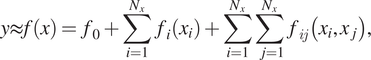 $$ y\approx f(x)={f}_0+\sum_{i=1}^{N_x}{f}_i\left({x}_i\right)+\sum_{i=1}^{N_x}\sum_{j=1}^{N_x}{f}_{ij}\left({x}_i,{x}_j\right),\kern1.00em $$
where  $ {N}_x $
is the dimension of the input space and
$ {N}_x $
is the dimension of the input space and  $ {f}_0 $
represents the mean value of
$ {f}_0 $
represents the mean value of  $ f(x) $
. The above approximation is sufficient in many situations in practice since terms containing functions of more than two input parameters can often be ignored due to their negligible contributions compared to the lower-order terms (Li et al., Reference Li, Wang and Rabitz2002). The terms in Equation (1) can be evaluated by approximating the functions
$ f(x) $
. The above approximation is sufficient in many situations in practice since terms containing functions of more than two input parameters can often be ignored due to their negligible contributions compared to the lower-order terms (Li et al., Reference Li, Wang and Rabitz2002). The terms in Equation (1) can be evaluated by approximating the functions  $ {f}_i\left({x}_i\right) $
and
$ {f}_i\left({x}_i\right) $
and  $ {f}_{ij}\left({x}_i,{x}_j\right) $
with some orthonormal basis functions,
$ {f}_{ij}\left({x}_i,{x}_j\right) $
with some orthonormal basis functions,  $ {\phi}_k\left({x}_i\right) $
, that can be easily computed. Popular choices for the basis functions include ordinary polynomials (Li et al., Reference Li, Wang and Rabitz2002) and Lagrange polynomials (Baran and Bieniasz, Reference Baran and Bieniasz2015). Apart from applications in chemical kinetics, HDMR has been applied in process engineering (Sikorski et al., Reference Sikorski, Brownbridge, Garud, Mosbach, Karimi and Kraft2016) and also in engine emissions modeling (Lai et al., Reference Lai, Parry, Mosbach, Bhave and Page2018).
$ {\phi}_k\left({x}_i\right) $
, that can be easily computed. Popular choices for the basis functions include ordinary polynomials (Li et al., Reference Li, Wang and Rabitz2002) and Lagrange polynomials (Baran and Bieniasz, Reference Baran and Bieniasz2015). Apart from applications in chemical kinetics, HDMR has been applied in process engineering (Sikorski et al., Reference Sikorski, Brownbridge, Garud, Mosbach, Karimi and Kraft2016) and also in engine emissions modeling (Lai et al., Reference Lai, Parry, Mosbach, Bhave and Page2018).
2.2. Deep neural networks
Deep learning, or deep ANNs, are composed of multiple processing layers to learn a representation of data with multiple levels of abstraction (LeCun et al., Reference LeCun, Bengio and Hinton2015). Deep learning has gained exploding popularity in the machine learning community over the past two decades, and it has been applied in numerous fields including computer vision, natural language processing, recommendation systems, and so forth, due to its ability to find both low- and high-level features of the data as well as its scalability to high-dimensional input spaces. However, the construction of deep learning requires specification of many hyperparameters including number of epochs, regularization strength, dropout rate, and so forth, and there is no universal paradigm for determining the optimal settings for these hyperparameters. Hence the performance of a DNN can heavily depend on engineering techniques such as architecture specification and parameter tuning.
In our study, we are only concerned with fully connected neural networks. The goal of a neural network is to learn the underlying representation of the given datasets. A deep feedforward network follows the standard forward propagation and backpropagation to tune the learnable parameters of the neural network, then use the trained network for further predictions on similar problems. In Figures 1 and 2, we show simple graphical representations for forward and backpropagation in a fully connected network, respectively.
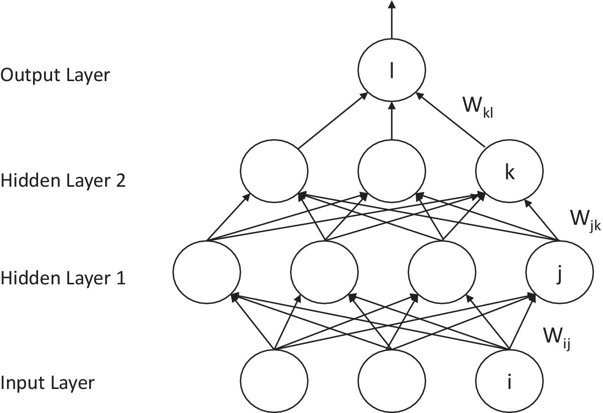
Figure 1. Forward propagation in a three-layer feedforward neural network. For each unit in the layers other than the input layer, the output of the unit equals the inner product between all the outputs from the previous layer and the weights followed by a nonlinearity (e.g., the ReLU function).
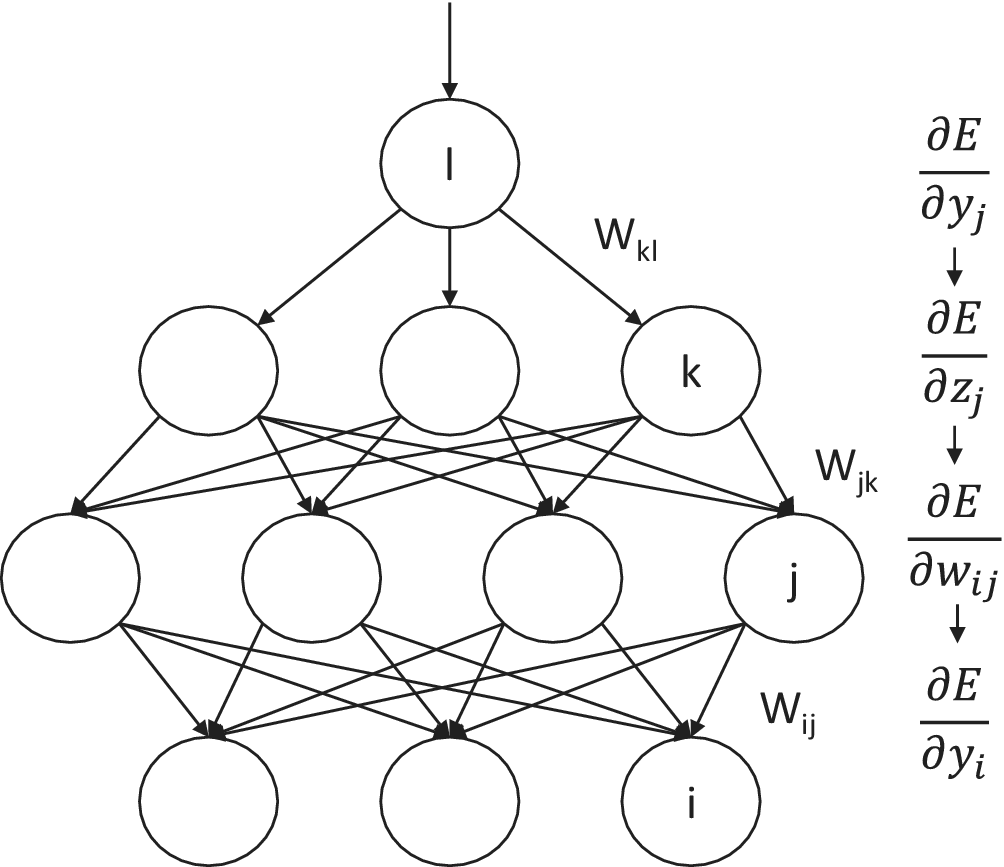
Figure 2. Backpropagation in a three-layer feedforward neural network. Computing the derivatives of the cost function with respect to the weight parameters using chain rules, then the parameters are updated using gradient descent with the computed derivatives.
The architecture of a neural network can be described as a directed graph whose vertices are called neurons, or nodes, and directed edges, each of which has an associated weight. The set of nodes with no incoming edges are called input nodes, whereas the nodes with no outgoing edges are called output nodes. We define the first layer to be the input layer and the last layer to be the output layer, and all other layers in between are called the hidden layers. The input data are propagated in a feedforward fashion as follows:
Figure 1 shows how input signals are propagated forward in a three-layer fully connected neural network, where for each unit in any layer other than the input layer, the input to the unit equals the inner product between the output signals from all the units from the previous layer and the associated weights:
 $$ {\displaystyle \begin{array}{ccc}{z}_j=\sum_{i\in \mathrm{previous}\ \mathrm{layer}}{w}_{ij}{y}_i.& & \end{array}} $$
The unit then outputs a scalar by applying a nonlinearity,  $ g $
, to this inner product:
$ g $
, to this inner product:  $ {y}_j=g\left({z}_j\right) $
. The signals are propagated forward in this way layer by layer until the output layer is reached. Commonly used nonlinear activation functions include the rectified linear unit (ReLU)
$ {y}_j=g\left({z}_j\right) $
. The signals are propagated forward in this way layer by layer until the output layer is reached. Commonly used nonlinear activation functions include the rectified linear unit (ReLU)  $ f(z)=\max \left(0,z\right) $
, the sigmoid function
$ f(z)=\max \left(0,z\right) $
, the sigmoid function  $ \sigma (z)={\left[1+\exp \left(-z\right)\right]}^{-1} $
and the hyperbolic tangent function
$ \sigma (z)={\left[1+\exp \left(-z\right)\right]}^{-1} $
and the hyperbolic tangent function  $ \tanh (z) $
. In this case, we have omitted bias terms for simplicity.
$ \tanh (z) $
. In this case, we have omitted bias terms for simplicity.
At an output node, after taking the linear combination of its predecessor values, instead of applying an activation function, an output rule can be used to aggregate the information across all the output nodes. In a regression problem, as opposed to a classification problem, we simply keep the linear combination as the output prediction.
The weights and bias parameters in neural networks are usually learnt via backpropagation using the cached quantities from the forward propagation stage. Backpropagation, as represented in Figure 2, is executed using gradient-descent–based optimization methods. Given a cost function,  $ E\left(\hat{y},y\right) $
, which quantifies the difference between the current predictions of the output (
$ E\left(\hat{y},y\right) $
, which quantifies the difference between the current predictions of the output ( $ \hat{y}\Big) $
and the actual outputs (
$ \hat{y}\Big) $
and the actual outputs ( $ y $
), the derivatives of
$ y $
), the derivatives of  $ E $
with respect to each weight in each layer of the network can be derived using the chain rule,
$ E $
with respect to each weight in each layer of the network can be derived using the chain rule,
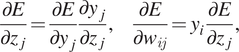 $$ {\displaystyle \begin{array}{ccc}\frac{\partial E}{\partial {z}_j}=\frac{\partial E}{\partial {y}_j}\frac{\partial {y}_j}{\partial {z}_j},\kern1.25em \frac{\partial E}{\partial {w}_{ij}}={y}_i\frac{\partial E}{\partial {z}_j},& & \end{array}} $$
where the initial  $ \partial E/ \partial {y}_j $
is derived given the activation function and the cost function. Then we compute
$ \partial E/ \partial {y}_j $
is derived given the activation function and the cost function. Then we compute  $ \partial E/ \partial {z}_j $
,
$ \partial E/ \partial {z}_j $
,  $ \partial E/ \partial {w}_{ij} $
and
$ \partial E/ \partial {w}_{ij} $
and  $ \partial E/ \partial {y}_i $
iteratively for each node
$ \partial E/ \partial {y}_i $
iteratively for each node  $ i $
in layer
$ i $
in layer  $ l $
and node
$ l $
and node  $ j $
in layer
$ j $
in layer  $ l-1 $
until we reach the input layer. Then we use methods such as stochastic gradient descent to update the weights in the network:
$ l-1 $
until we reach the input layer. Then we use methods such as stochastic gradient descent to update the weights in the network:
 $$ {\displaystyle \begin{array}{ccc}{w}_{ij}\leftarrow {w}_{ij}-\alpha \frac{\partial E}{\partial {w}_{ij}},& & \end{array}} $$
where  $ \alpha $
is some scalar known as the learning rate.
$ \alpha $
is some scalar known as the learning rate.
Iterative application of forward propagation and backpropagation will gradually decrease the cost function value in general, and if the cost function is convex in the input space, it will eventually converge to the global minimum or somewhere close to the global minimum.
The power of neural networks lies in the composition of the nonlinear activation functions. From the results on universal approximation bounds for superpositions of the sigmoid function by Barron (Reference Barron1993), it can be implied that a neural network with sigmoid activation can arbitrarily closely approximate a nonparametric regression mode.
Here we only discuss fully connected neural networks, where the only learnable parameters are the weight parameters  $ {w}_{ij} $
between each node
$ {w}_{ij} $
between each node  $ i $
in layer
$ i $
in layer  $ l-1 $
and each node
$ l-1 $
and each node  $ j $
in the previous layer
$ j $
in the previous layer  $ l $
. For a general review of various architectures of deep learning such as convolutional neural networks and recurrent neural networks, the reader is referred to LeCun et al. (Reference LeCun, Bengio and Hinton2015) for example.
$ l $
. For a general review of various architectures of deep learning such as convolutional neural networks and recurrent neural networks, the reader is referred to LeCun et al. (Reference LeCun, Bengio and Hinton2015) for example.
2.3. Gaussian processes
A GP is a stochastic process, which is a collection of random variables, with the property that any finite subcollection of the random variables have a joint multivariate Gaussian distribution (Williams and Rasmussen, Reference Williams and Rasmussen2006). We denote the fact that a stochastic process  $ f\left(\cdot \right) $
is a GP with mean function
$ f\left(\cdot \right) $
is a GP with mean function  $ m\left(\cdot \right) $
and covariance function
$ m\left(\cdot \right) $
and covariance function  $ k\left(\cdot, \cdot \right) $
as
$ k\left(\cdot, \cdot \right) $
as
 $$ {\displaystyle \begin{array}{ccc}f\left(\cdot \right)\sim \mathbf{\mathcal{GP}}\left(m\left(\cdot \right),k\left(\cdot, \cdot \right)\right).& & \end{array}} $$
The definition implies that for any  $ {x}^{(1)},{x}^{(2)},\dots, {x}^{(n)}\in \mathbf{\mathcal{X}} $
, where
$ {x}^{(1)},{x}^{(2)},\dots, {x}^{(n)}\in \mathbf{\mathcal{X}} $
, where  $ \mathbf{\mathcal{X}} $
denotes the set of possible inputs, we have
$ \mathbf{\mathcal{X}} $
denotes the set of possible inputs, we have
 $$ {\displaystyle \begin{array}{ccc}{\left[f\left({x}^{(1)}\right),\dots, f\left({x}^{(n)}\right)\right]}^{\mathrm{T}}\sim \mathbf{\mathcal{N}}\left({\left[m\left({x}^{(1)}\right),\dots, m\left({x}^{(n)}\right)\right]}^{\mathrm{T}},K\right),& & \end{array}} $$
where the covariance matrix  $ K $
has entries
$ K $
has entries  $ {K}_{ij}=k\left({x}^{(i)},{x}^{(j)}\right) $
.
$ {K}_{ij}=k\left({x}^{(i)},{x}^{(j)}\right) $
.
GPs can be interpreted as a natural extension of multivariate Gaussian distributions to have infinite index sets, and this extension allows us to think of a GP as a distribution over random functions. A GP is fully determined by its mean and covariance functions. The mean function can be any real-valued function, whereas the covariance function has to satisfy that the resulting covariance matrix  $ K $
for any set of inputs
$ K $
for any set of inputs  $ {x}^{(1)},\dots, {x}^{(n)}\in \mathbf{\mathcal{X}} $
has to be a valid covariance matrix for a multivariate Gaussian distribution, which implies that
$ {x}^{(1)},\dots, {x}^{(n)}\in \mathbf{\mathcal{X}} $
has to be a valid covariance matrix for a multivariate Gaussian distribution, which implies that  $ K $
has to be positive semidefinite and this criterion corresponds to Mercer’s condition for kernels (Minh et al., Reference Minh, Niyogi and Yao2006). Hence the covariance function is sometimes also known as the kernel function. One of the most popular choices of kernel function is the RBF (or squared error) kernel
$ K $
has to be positive semidefinite and this criterion corresponds to Mercer’s condition for kernels (Minh et al., Reference Minh, Niyogi and Yao2006). Hence the covariance function is sometimes also known as the kernel function. One of the most popular choices of kernel function is the RBF (or squared error) kernel
 $$ {\displaystyle \begin{array}{ccc}{k}_{\mathsf{RBF}}\left(x,{x}^{\prime}\right)=\exp \left(-\frac{\parallel x-{x}^{\prime }{\parallel}^2}{2{l}^2}\right),& & \end{array}} $$
where  $ l $
is a kernel parameter which quantifies the level of local smoothness of the distribution drawn from the GP.
$ l $
is a kernel parameter which quantifies the level of local smoothness of the distribution drawn from the GP.
GPs have gained increasing popularity in the machine learning community since Neal (Reference Neal1996) showed that Bayesian neural networks with infinitely many nodes converge to GPs with a certain kernel function. Therefore, GPs can be viewed as a probabilistic and interpretable alternative to neural networks.
In our study, the focus of the application of GPs lies within regression tasks. Suppose we are given a dataset  $ \mathbf{\mathcal{D}}={\left\{{x}^{(i)},{y}^{(i)}\right\}}_{i=1,\dots, n} $
, that one may refer to as the training set, of independent samples from some unknown distribution, where
$ \mathbf{\mathcal{D}}={\left\{{x}^{(i)},{y}^{(i)}\right\}}_{i=1,\dots, n} $
, that one may refer to as the training set, of independent samples from some unknown distribution, where  $ {x}^{(i)}\in {\mathbb{R}}^d $
and
$ {x}^{(i)}\in {\mathbb{R}}^d $
and  $ {y}^{(i)}\in \mathbb{R} $
for
$ {y}^{(i)}\in \mathbb{R} $
for  $ i=1,\dots, n $
. A GP regression model is then
$ i=1,\dots, n $
. A GP regression model is then
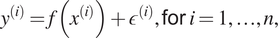 $$ {\displaystyle \begin{array}{ccc}{y}^{(i)}=f\left({x}^{(i)}\right)+{\epsilon}^{(i)},\mathsf{for}\ i=1,\dots, n,& & \end{array}} $$
with a GP prior over the functions  $ f $
, that is
$ f $
, that is  $ f\left(\cdot \right)\sim \mathbf{\mathcal{GP}}\left(m\left(\cdot \right),k\left(\cdot, \cdot \right)\right) $
, for some mean function
$ f\left(\cdot \right)\sim \mathbf{\mathcal{GP}}\left(m\left(\cdot \right),k\left(\cdot, \cdot \right)\right) $
, for some mean function  $ m\left(\cdot \right) $
and valid kernel function
$ m\left(\cdot \right) $
and valid kernel function  $ k\left(\cdot, \cdot \right) $
, and the
$ k\left(\cdot, \cdot \right) $
, and the  $ {\epsilon}^{(i)} $
are independent additive Gaussian noises that follow
$ {\epsilon}^{(i)} $
are independent additive Gaussian noises that follow  $ \mathbf{\mathcal{N}}\left(0,{\sigma}^2\right) $
distributions.
$ \mathbf{\mathcal{N}}\left(0,{\sigma}^2\right) $
distributions.
Suppose we are given another dataset  $ {\mathbf{\mathcal{D}}}_{\ast }={\left\{{x}_{\ast}^{(i)},{y}_{\ast}^{(i)}\right\}}_{i=1,\dots, {n}_{\ast }} $
, that one may refer to as the blind-test set, drawn from the same distribution as
$ {\mathbf{\mathcal{D}}}_{\ast }={\left\{{x}_{\ast}^{(i)},{y}_{\ast}^{(i)}\right\}}_{i=1,\dots, {n}_{\ast }} $
, that one may refer to as the blind-test set, drawn from the same distribution as  $ \mathbf{\mathcal{D}} $
. By the definition of a GP, we have
$ \mathbf{\mathcal{D}} $
. By the definition of a GP, we have
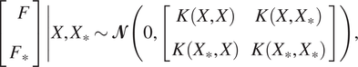 $$ {\displaystyle \begin{array}{ccc}\left[\begin{array}{c}F\\ {}{F}_{\ast}\end{array}\right]\left|X,{X}_{\ast}\sim \mathbf{\mathcal{N}}\left(0,\left[\begin{array}{cc}K\left(X,X\right)& K\left(X,{X}_{\ast}\right)\\ {}K\left({X}_{\ast },X\right)& K\left({X}_{\ast },{X}_{\ast}\right)\end{array}\right]\right),\right.& & \end{array}} $$
where  $ X={\left\{{x}^{(i)}\right\}}_{i=1,\dots, n} $
,
$ X={\left\{{x}^{(i)}\right\}}_{i=1,\dots, n} $
,  $ F $
represents
$ F $
represents  $ {\left[f\left({x}^{(1)}\right),\dots, f\left({x}^{(n)}\right)\right]}^{\top } $
,
$ {\left[f\left({x}^{(1)}\right),\dots, f\left({x}^{(n)}\right)\right]}^{\top } $
,  $ K\left(X,X\right) $
represents an
$ K\left(X,X\right) $
represents an  $ n\times n $
kernel matrix whose
$ n\times n $
kernel matrix whose  $ \left(i,j\right) $
entry is
$ \left(i,j\right) $
entry is  $ K\left({x}^{(i)},{x}^{(j)}\right) $
, and analogous definitions for quantities with asterisk subscripts, for example,
$ K\left({x}^{(i)},{x}^{(j)}\right) $
, and analogous definitions for quantities with asterisk subscripts, for example,  $ {X}_{\ast }={\left\{{x}_{\ast}^{(i)}\right\}}_{i=1,\dots, {n}_{\ast }} $
. Then, given the additive Gaussian noises, the joint distribution of
$ {X}_{\ast }={\left\{{x}_{\ast}^{(i)}\right\}}_{i=1,\dots, {n}_{\ast }} $
. Then, given the additive Gaussian noises, the joint distribution of  $ Y={\left[{y}^{(1)},\dots, {y}^{(n)}\right]}^{\top } $
and
$ Y={\left[{y}^{(1)},\dots, {y}^{(n)}\right]}^{\top } $
and  $ {Y}_{\ast } $
becomes
$ {Y}_{\ast } $
becomes $ {\displaystyle \begin{array}{ccc}& & \end{array}} $
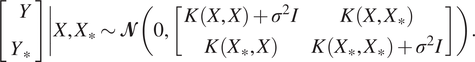 $$ \left[\begin{array}{c}Y\\ {}{Y}_{\ast}\end{array}\right]\left|X,{X}_{\ast}\sim \mathbf{\mathcal{N}}\left(0,\left[\begin{array}{cc}K\left(X,X\right)+{\sigma}^2I& K\left(X,{X}_{\ast}\right)\\ {}K\left({X}_{\ast },X\right)& K\left({X}_{\ast },{X}_{\ast}\right)+{\sigma}^2I\end{array}\right]\right)\right.. $$
Using the rules for conditioning Gaussian distributions, the posterior distribution of the blind-test data given the training data is then given by
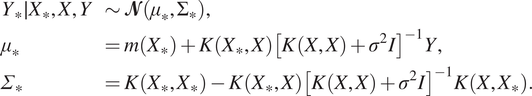 $$ {\displaystyle \begin{array}{llll}{Y}_{\ast}\mid {X}_{\ast },X,Y& \sim \mathbf{\mathcal{N}}\left({\mu}_{\ast },{\Sigma}_{\ast}\right),& & \\ {}{\mu}_{\ast }& =m\left({X}_{\ast}\right)+K\left({X}_{\ast },X\right){\left[K\left(X,X\right)+{\sigma}^2I\right]}^{-1}Y,& & \\ {}{\varSigma}_{\ast }& =K\left({X}_{\ast },{X}_{\ast}\right)-K\left({X}_{\ast },X\right){\left[K\left(X,X\right)+{\sigma}^2I\right]}^{-1}K\left(X,{X}_{\ast}\right).& & \end{array}} $$
Equation (11) is the posterior GP regression model for predictions. The kernel parameters  $ \theta $
of the kernel function in the GP regression model can be learnt by maximizing the (log) posterior marginal likelihood
$ \theta $
of the kernel function in the GP regression model can be learnt by maximizing the (log) posterior marginal likelihood
 $$ {\displaystyle \begin{array}{ccc}\log\ p\left(Y|\theta, X\right)\propto -{Y}^{\top }{\left({K}_{\theta}\left(X,X\right)+{\sigma}^2I\right)}^{-1}\mathrm{Y}-\log \left|{K}_{\theta}\left(X,X\right)+{\sigma}^2I\right|& & \end{array}} $$
with respect to the kernel parameters, where we have emphasized the dependence of the kernel matrix  $ K $
on its parameters
$ K $
on its parameters  $ \theta $
through a subscript.
$ \theta $
through a subscript.
2.4. Deep kernel learning
We now briefly discuss the main method we apply as a surrogate model, DKL (Wilson et al., Reference Wilson, Hu, Salakhutdinov and Xing2016). DKL can be intuitively interpreted as a combination of a DNN and a GP. A graphical representation of a DKL model is shown in Figure 3, where we can see that the structure consists of a DNN followed by a GP. As mentioned in the previous section, a GP is the limit of a Bayesian neural network with an infinite number of nodes, hence the GP at the end of the DKL architecture can be interpreted as another hidden layer in the DNN, but with an infinite number of nodes, and this greatly increases the expressiveness compared to a stand-alone DNN. When the data enters the DKL model, it is first propagated in a forward fashion through the neural network. The high-dimensional input data is thus transformed by the neural network into a lower-dimensional feature vector, which is then used as the input arguments for GP regression. The expectation of the resulting posterior distribution is then taken as the value predicted by DKL as a function of the input data. As GPs naturally do not perform well in high-dimensional input spaces, the DNN acts as a feature extractor and dimensionality reduction method for more robust GP regression. Being a combination of deep learning and kernel learning, DKL encapsulates the expressive power for extracting high-level features and capturing nonstationary structures within the data given its deep architectures and the nonparametric flexibility in kernel learning induced by its probabilistic GP framework.
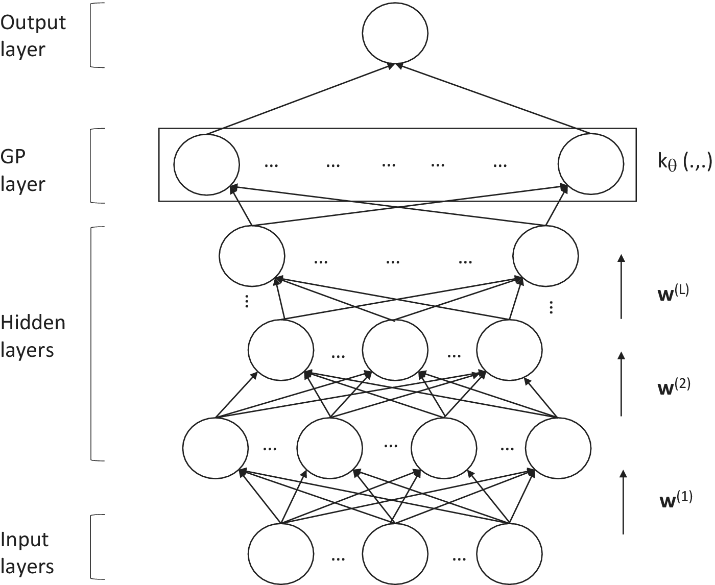
Figure 3. Deep kernel learning: input data is propagated in a forward fashion through the hidden layers of the neural network parameterized by the weight parameters. Then, the low-dimensional high-level feature vector as the output of the neural network is fed into a GP with a base kernel function  $ {k}_{\theta}\left(\cdot, \cdot \right) $
for regression. The posterior mean of the Gaussian regression model is taken as the prediction given the input data (Adapted from Wilson et al., Reference Wilson, Hu, Salakhutdinov and Xing2016).
$ {k}_{\theta}\left(\cdot, \cdot \right) $
for regression. The posterior mean of the Gaussian regression model is taken as the prediction given the input data (Adapted from Wilson et al., Reference Wilson, Hu, Salakhutdinov and Xing2016).
We can also view DKL as a GP with a stand-alone deep kernel. Starting from a base kernel  $ k\left({x}^{(i)},{x}^{(j)}|\theta \right) $
with kernel parameters, the deep kernel can be constructed as
$ k\left({x}^{(i)},{x}^{(j)}|\theta \right) $
with kernel parameters, the deep kernel can be constructed as
 $$ {\displaystyle \begin{array}{ccc}k\left({x}^{(i)},{x}^{(j)}|\theta \right)\to k\left(g\left({x}^{(i)},w\right),g\Big({x}^{(j)},w\Big)|\theta, w\right),& & \end{array}} $$
where  $ g\left(x;w\right) $
is a nonlinear mapping induced by the neural network with weight parameters
$ g\left(x;w\right) $
is a nonlinear mapping induced by the neural network with weight parameters  $ w $
. A popular choice for the base kernel
$ w $
. A popular choice for the base kernel  $ k\left({x}^{(i)},{x}^{(j)}|\theta \right) $
is again the RBF kernel (Equation 7). Inspired by Wilson et al. (Reference Wilson, Hu, Salakhutdinov and Xing2016), we also look at the spectral mixture (SM) base kernel
$ k\left({x}^{(i)},{x}^{(j)}|\theta \right) $
is again the RBF kernel (Equation 7). Inspired by Wilson et al. (Reference Wilson, Hu, Salakhutdinov and Xing2016), we also look at the spectral mixture (SM) base kernel
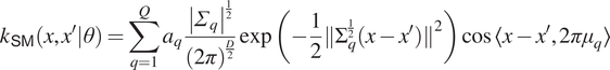 $$ {\displaystyle \begin{array}{ccc}{k}_{\mathsf{SM}}\left(x,{x}^{\prime }|\theta \right)=\sum_{q=1}^Q{a}_q\frac{{\left|{\varSigma}_q\right|}^{\frac{1}{2}}}{{\left(2\pi \right)}^{\frac{D}{2}}}\exp \left(-\frac{1}{2}{\left\Vert \Sigma \right.}_q^{\frac{1}{2}}{\left.\left(x-{x}^{\prime}\right)\right\Vert}^2\right)\cos \left\langle x-{x}^{\prime },2\pi {\mu}_q\right\rangle & & \end{array}} $$
by Wilson and Adams (Reference Wilson and Adams2013), where the learnable kernel parameters  $ \theta =\left\{{a}_q,{\Sigma}_q,{\mu}_q\right\} $
consist of a weight, an inverse length scale, and a frequency vector for each of the
$ \theta =\left\{{a}_q,{\Sigma}_q,{\mu}_q\right\} $
consist of a weight, an inverse length scale, and a frequency vector for each of the  $ Q $
spectral components, and where
$ Q $
spectral components, and where  $ \left\langle \cdot, \cdot \right\rangle $
denotes the standard inner product. The spectral mixture kernel is meant to be able to represent quasi-periodic stationary structures within the data.
$ \left\langle \cdot, \cdot \right\rangle $
denotes the standard inner product. The spectral mixture kernel is meant to be able to represent quasi-periodic stationary structures within the data.
We denote by  $ \gamma =\left\{w,\theta \right\} $
the parameters of the DKL model, consisting of the neural network weight parameters
$ \gamma =\left\{w,\theta \right\} $
the parameters of the DKL model, consisting of the neural network weight parameters  $ w $
and the GP kernel parameters. These parameters are learnt jointly via maximizing the log-posterior marginal likelihood of the GP (Equation 12) with respect to.
$ w $
and the GP kernel parameters. These parameters are learnt jointly via maximizing the log-posterior marginal likelihood of the GP (Equation 12) with respect to.
3. Applying DKL to engine emissions
3.1. Dataset
The dataset used in this work was obtained from a diesel-fueled compression ignition engine whose main geometric features are provided in Table 1. The data consists of soot and NOx emissions taken engine-out during steady-state operation at 1,861 distinct operating points. Each of these points is characterized by 14 operating condition variables, which include engine speed and torque, intake manifold temperature, injection pressure, mass fraction of recirculated exhaust gas, start, end, and fuel mass of injection, and combustion chamber wall temperatures. The set of points is spread roughly evenly over the entire engine operating window in terms of speed and load. NOx emissions are measured in units of parts per million by volume (ppmv) with a nominal error bar of 3% and soot represent the carbon fraction of emitted particulate matter with a stated measurement uncertainty of 5%.
Table 1. Specification of the turbocharged four-stroke diesel-fueled compression ignition engine used in this work.
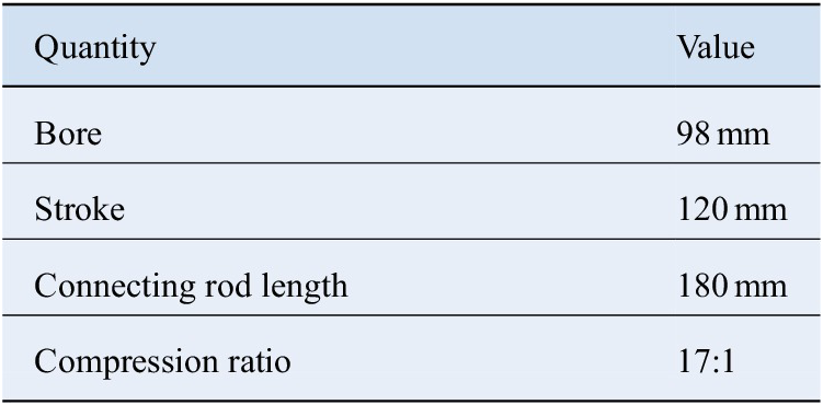
Since the numerical values of the soot response vary over several orders of magnitude, it is necessary to consider their logarithms instead of their raw values. The NOx response values can be used as is. We split the dataset randomly into disjoint training and blind-test sets, which comprise 90% and 10% of the total, respectively.
3.2. Implementation
In all numerical experiments, our DKL implementation consists of a five-layer fully connected network and a GP with RBF kernel. The neural network employs the rectified linear unit (ReLU) function LeCun et al. (Reference LeCun, Bengio and Hinton2015) as the activation function for each hidden layer, and all the weights are initialized with the He normal initialization (He et al., Reference He, Zhang, Ren and Sun2015). We use the standard root mean squared error (RMSE) loss function, and the Adam optimizer for optimization (Kingma and Ba, Reference Kingma and Ba2014).
We implement DKL as a surrogate model into model development suite (MoDS) (CMCL Innovations, 2018)—an integrated software written in C++ with multiple tools for conducting various generic tasks to develop black-box models. Such tasks include surrogate model creation (Sikorski et al., Reference Sikorski, Brownbridge, Garud, Mosbach, Karimi and Kraft2016), parameter estimation (Kastner et al., Reference Kastner, Braumann, Man, Mosbach, Brownbridge, Akroyd, Kraft and Himawan2013), error propagation (Mosbach et al., Reference Mosbach, Hong, Brownbridge, Kraft, Gudiyella and Brezinsky2014), and experimental design (Mosbach et al., Reference Mosbach, Braumann, Man, Kastner, Brownbridge and Kraft2012). Our MoDS-implementation of DKL uses PyTorch (Paszke et al., Reference Paszke, Gross, Chintala, Chanan, Yang, DeVito, Lin, Desmaison, Antiga and Lerer2017) and GPyTorch (Gardner et al., Reference Gardner, Pleiss, Weinberger, Bindel and Wilson2018).
All simulations were performed on a desktop PC with 12 3.2 GHz CPU-cores and 16 GB RAM. Even though MoDS allows parallel execution, all simulations were conducted in serial in order to simplify quantification of computational effort. For the same reason, no GPU-acceleration of Torch-based code was considered. We also did not explore the use of kernel interpolation techniques (Wilson and Nickisch, Reference Wilson and Nickisch2015; Quiñonero-Candela and Rasmussen, Reference Quiñonero-Candela and Rasmussen2005) to speed up GP learning.
3.3. Network architecture, kernel, and learning parameters
The DKL framework involves learnable parameters such as network weights and kernel parameters, as well as hyperparameters such as the learning rate, number of iterations, and number of nodes in each layer of the neural network. Before training can be carried out, suitable values of the hyperparameters need to be chosen. We approach this in two ways: First, we make this choice manually, based on previous experience and cross-validation over a small hyperparameter search-space, and second, we employ a systematic, optimization-based procedure. In both cases, we determine the following seven hyperparameters: the number of nodes in each of the four hidden layers, the prior white-noise level of the GP, the number of epochs, that is training iterations, and the learning rate.
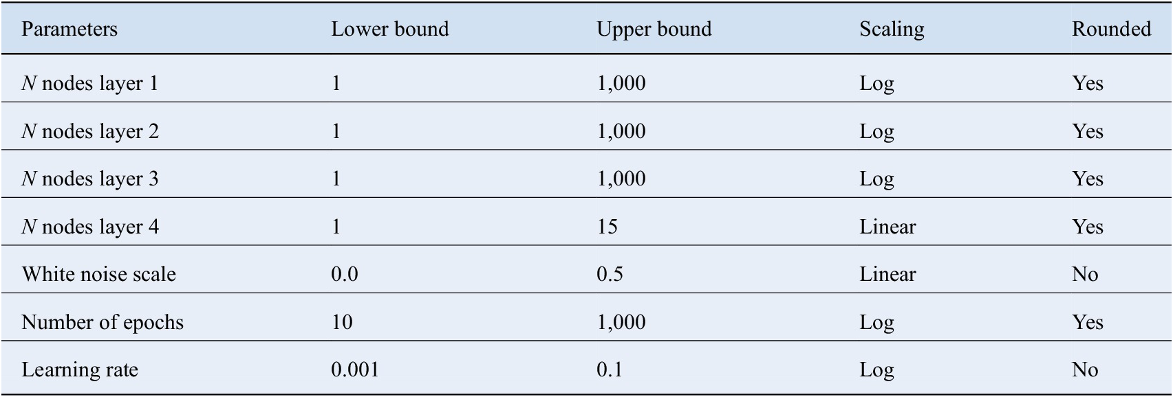
The optimization approach consists of two stages: a global quasi-random search followed by a local optimization with a gradient-free grid-based method, both of which are conducted using MoDS. For the first stage, a Sobol sequence (Joe and Kuo, Reference Joe and Kuo2008), a low-discrepancy sampling method, is employed. We generate 1,000 Sobol points within the space spanned by all of the hyperparameters given in Table 2, which also provides the range and scaling type for each parameter. We then fit the DKL under each of these 1,000 hyperparameter settings to the training data. The quality of each fit is assessed by calculating the objective function
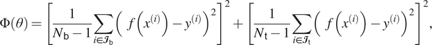 $$ {\displaystyle \begin{array}{ccc}\Phi \left(\theta \right)={\left[\frac{1}{N_{\mathsf{b}}-1}\sum_{i\in {\mathbf{\mathcal{I}}}_{\mathsf{b}}}{\left(f\left({x}^{(i)}\right)-{y}^{(i)}\right)}^2\right]}^2+{\left[\frac{1}{N_{\mathsf{t}}-1}\sum_{i\in {\mathbf{\mathcal{I}}}_{\mathsf{t}}}{\left(f\left({x}^{(i)}\right)-{y}^{(i)}\right)}^2\right]}^2,& & \end{array}} $$
Table 2. Deep kernel learning hyperparameters considered for optimization.
where  $ f $
denotes the surrogate model, that is, the trained DKL, and
$ f $
denotes the surrogate model, that is, the trained DKL, and  $ {x}^{(i)} $
and
$ {x}^{(i)} $
and  $ {y}^{(i)} $
the experimental operating conditions and responses (soot or NOx), respectively, of the
$ {y}^{(i)} $
the experimental operating conditions and responses (soot or NOx), respectively, of the  $ i\mathrm{th} $
data point.
$ i\mathrm{th} $
data point.  $ {\mathbf{\mathcal{I}}}_{\mathsf{b}} $
denotes the set of indices belonging to the blind-test data points, and
$ {\mathbf{\mathcal{I}}}_{\mathsf{b}} $
denotes the set of indices belonging to the blind-test data points, and  $ {N}_{\mathsf{b}} $
denotes their number, whereas
$ {N}_{\mathsf{b}} $
denotes their number, whereas  $ {\mathbf{\mathcal{I}}}_{\mathsf{t}} $
and
$ {\mathbf{\mathcal{I}}}_{\mathsf{t}} $
and  $ {N}_{\mathsf{t}} $
refer to the analogous quantities for the training data points. The normalization of the two parts of the objective function, that is, the training and blind-test parts, by the number of points they contain, implies that the two parts are equally weighted with respect to each another, irrespective of how many points they contain. We tested other forms of the objective function but found empirically that this form yields the best results. Furthermore, we note that including the blind-test points into the objective function is not a restriction. In any application, whatever set of points is given, it can arbitrarily be split into training and blind-test subsets. Again, we made this choice because we found empirically that it produces the best results.
$ {N}_{\mathsf{t}} $
refer to the analogous quantities for the training data points. The normalization of the two parts of the objective function, that is, the training and blind-test parts, by the number of points they contain, implies that the two parts are equally weighted with respect to each another, irrespective of how many points they contain. We tested other forms of the objective function but found empirically that this form yields the best results. Furthermore, we note that including the blind-test points into the objective function is not a restriction. In any application, whatever set of points is given, it can arbitrarily be split into training and blind-test subsets. Again, we made this choice because we found empirically that it produces the best results.
Scatter plots of the Sobol points, showing their objective values against two of the architecture parameters, are given in Figure 4. In Figure 4a, we observe that best performance is achieved if the number of nodes in the first layer well exceeds the number of inputs. From Figure 4b, we conclude that the number of features extracted by the neural network part of DKL, that is, the number of nodes in the fourth hidden layer or in other words the number of quantities fed as input to the GP, for which the objective function attains its minimum is three. The objective value deteriorates appreciably for four and five features.
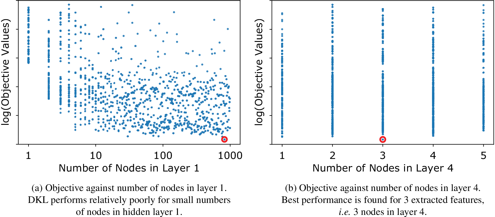
Figure 4. Combined training and blind-test objective function value (Equation 15) for 1,000 Sobol points in the space of hyperparameters of Table 2. The point with the lowest objective value overall is circled.
The best Sobol point as measured by Equation (15) (highlighted in Figure 4) is then optimized further with respect to the white noise of GP, number of epochs and learning rate using the algorithm by Hooke and Jeeves (Reference Hooke and Jeeves1961)—a gradient-free grid-based optimization algorithm, which is also part of MoDS. Since both the Sobol and Hooke–Jeeves method are designed for continuous variables, we treat the discrete parameters, that is, the number of nodes in each layer and the number of epochs, internally as continuous and simply round their values to the nearest integers when passing them on to DKL. This is also indicated in Table 2. Other optimization methods more suitable for discrete problems, such as genetic algorithms, are expected to perform at least as well, however, it is beyond the scope of the present work to explore this.
We note that the Hooke-Jeeves optimization step achieves only a relatively small improvement upon the best Sobol point, with the algorithm terminating after 68 and 78 iterations for NOx and soot, respectively. However, one should bear in mind that DKL training itself being based on stochastic optimization, and thus noise inherently being present in the quality of the fit, presents a challenge to any local optimization method. We furthermore find that there is little to no benefit in including the architecture parameters of the network, that is, the number of nodes in the hidden layers, into the Hooke-Jeeves optimization, so we excluded them from this stage.
The average CPU-time for (serial) evaluation of each Sobol or Hooke-Jeeves point was about 1 min for NOx and 2 min for soot. The reason for the larger evaluation time for soot is that the optimization favored a number of epochs on average about twice as high for soot as for NOx.
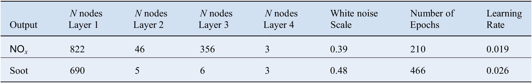
Table 3 shows the best values for the hyperparameters we find using the procedure described above. We note that due to the random nature of both the global search and the DKL training process itself, our procedure does not guarantee a global minimum.
Table 3. Best values found for the hyperparameters in deep kernel learning through optimization.
The best values found manually for the hyperparameters in DKL are 1000, 500, 50, and 3 for the numbers of nodes in the hidden layers, a white-noise level of 0.1, 200 training epochs, and a learning rate of 0.01.
3.4. Comparison
Figure 5 shows a comparison of model versus experiment using HDMR and DKL for both NOx and soot responses. For DKL, two sets of results are shown: One (Figure 5c,d) obtained using the best values for the hyperparameters found manually, and another one (Figure 5e,f) using the optimized values. The NOx values are scaled linearly, whereas the soot values are scaled logarithmically. The shaded areas in the plots represent an error margin of 20% with respect to the experimental values. We note that DKL generally produces more accurate regression fits for the data than HDMR for both NOx and soot, and also that DKL with the optimized hyperparameters is more accurate than with the manual ones. In the NOx regression with DKL, almost all of the predicted training and blind-test values lie within 20% of the experimental value and a large majority of the predictions align closely with the experimental values. For HDMR, although only few points lie outside the 20% margin, the predictions tend to be distributed further from the experimental values. For the soot regression, similar behavior is observed, but in this case, significantly more predictions lie outside the 20% error bar with respect to the experimental values. Soot being more challenging than NOx in terms of regression is entirely expected, due to soot emissions depending much more nonlinearly on the engine operating condition and the measurements being intrinsically much more noisy. In addition, we note in Figure 5 that the spread of training points is quite similar to that of the blind-test points for HDMR, whereas the latter is much wider for DKL, with the effect being stronger for soot than for NOx. These observations are quantified in Table 4 in terms of the percentage of points, which lie within 20% of the experimental values, as well as RSME. The blind-test RMSE is indeed seen to be larger than the training error for both NOx and soot regression, and the difference is larger in relative terms for soot. This is indicative of over-fitting—a well-known issue with neural networks (Srivastava et al., Reference Srivastava, Hinton, Krizhevsky, Sutskever and Salakhutdinov2014). Any surrogate with a large number of internal degrees of freedom is prone to over-fitting, especially if this number exceeds the number of data points. Given the number of layers and nodes typically used in a neural network, and hence the associated number of weights, it is clear that in our case the number of degrees of freedom in DKL is much larger than the number of available data points. Another factor contributing to over-fitting is the sparsity of the dataset in the input space, where there are less than  $ 2000 $
available training points in
$ 2000 $
available training points in  $ 14 $
dimensions. As an aside, an additional consequence of this sparsity is that the variances predicted by Equation (11) are too small to be useful, which is why they are not shown in any of the plots.
$ 14 $
dimensions. As an aside, an additional consequence of this sparsity is that the variances predicted by Equation (11) are too small to be useful, which is why they are not shown in any of the plots.
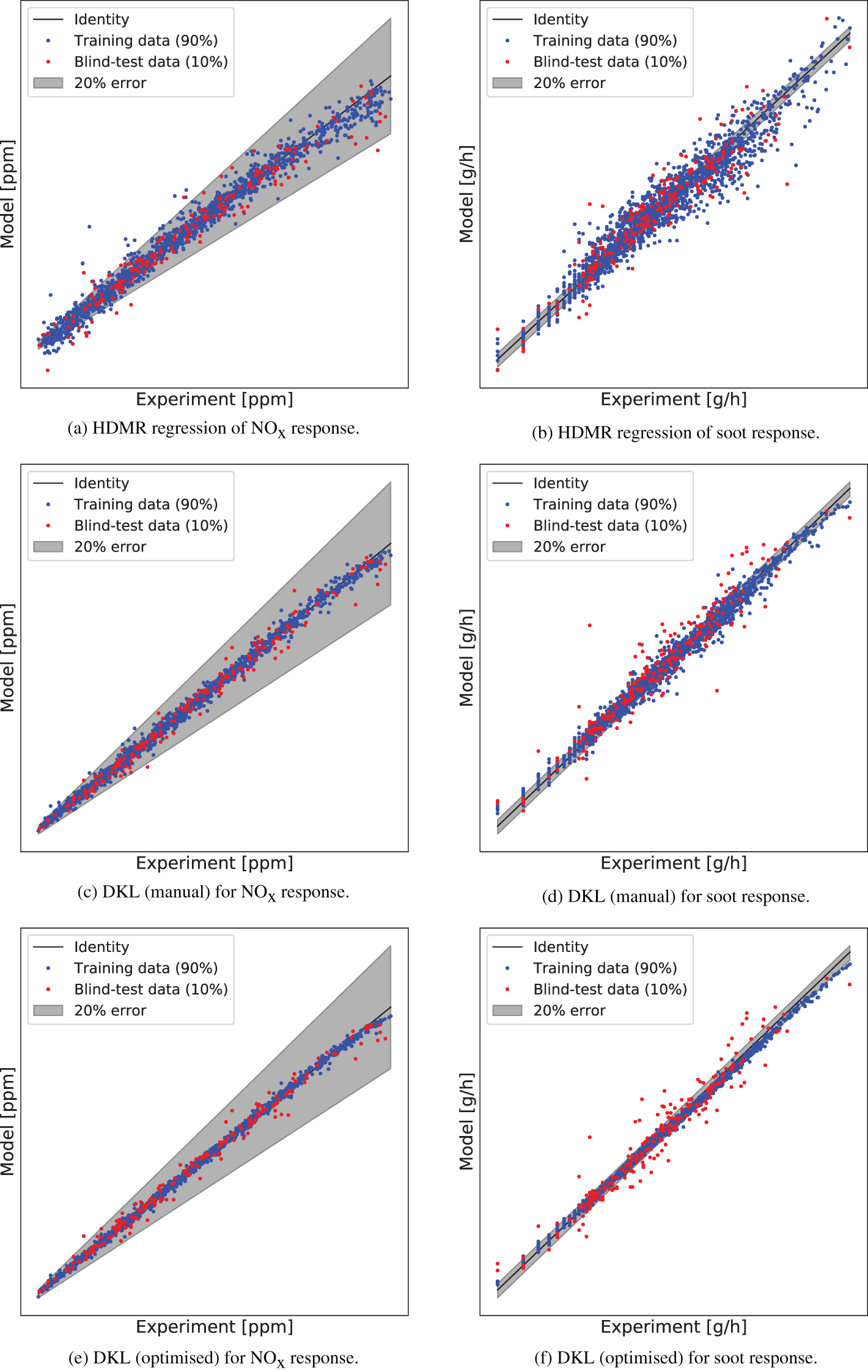
Figure 5. Modeled  $ {\mathsf{NO}}_x $
and soot responses against experimental ones using high-dimensional model representation (HDMR) and two sets of deep kernel learning (DKL) architectures and hyperparameter values. Soot values are logarithmic. For confidentiality reasons, no values are shown on the axes.
$ {\mathsf{NO}}_x $
and soot responses against experimental ones using high-dimensional model representation (HDMR) and two sets of deep kernel learning (DKL) architectures and hyperparameter values. Soot values are logarithmic. For confidentiality reasons, no values are shown on the axes.
Table 4. Percentage of predictions within 20% of the experimental value and root mean square errors (RSME) of  $ {\mathsf{NO}}_x $
and soot regressions for high-dimensional model representation (HDMR) and deep kernel learning (DKL).
$ {\mathsf{NO}}_x $
and soot regressions for high-dimensional model representation (HDMR) and deep kernel learning (DKL).
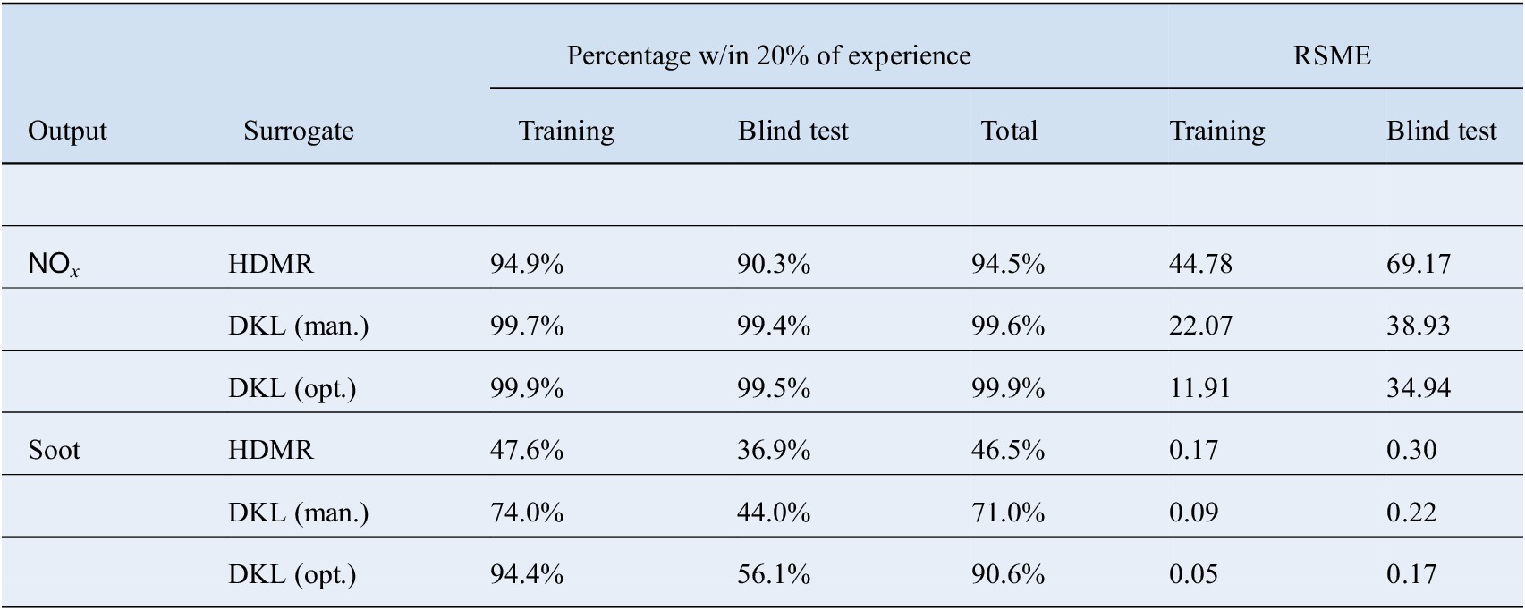
Figure 6 shows density plots of relative values  $ \hat{y}/ y $
for both outputs for DKL and HDMR, where
$ \hat{y}/ y $
for both outputs for DKL and HDMR, where  $ \hat{y} $
and
$ \hat{y} $
and  $ y $
represent the predicted and experimental values, respectively. It can be observed that for both outputs, the relative values for both HDMR and DKL are mainly distributed near unity, and the majority of the predicted values are within 20% of the experimental values for both methods for both outputs. However, it is clear from the plots that the overall distribution of errors of DKL is significantly more centralized at unity than HDMR for the regression of both outputs as the density is more centralized at unity for DKL than HDMR for both outputs. It is also clear that the number of predictions within 20% of the experimental value made by DKL is more than those made by HDMR, and this difference is greater for the soot prediction.
$ y $
represent the predicted and experimental values, respectively. It can be observed that for both outputs, the relative values for both HDMR and DKL are mainly distributed near unity, and the majority of the predicted values are within 20% of the experimental values for both methods for both outputs. However, it is clear from the plots that the overall distribution of errors of DKL is significantly more centralized at unity than HDMR for the regression of both outputs as the density is more centralized at unity for DKL than HDMR for both outputs. It is also clear that the number of predictions within 20% of the experimental value made by DKL is more than those made by HDMR, and this difference is greater for the soot prediction.
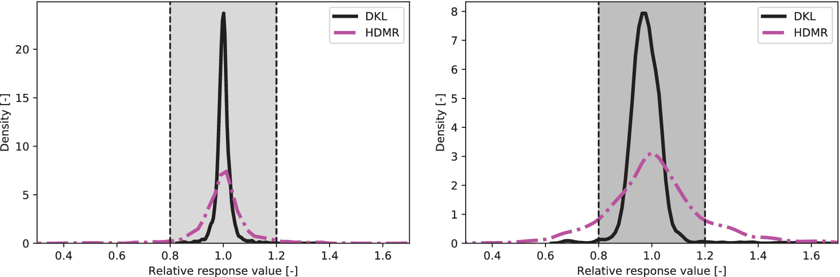
Figure 6. Densities of prediction values relative to experiment using high-dimensional model representation (HDMR) and deep kernel learning (DKL) regression for  $ {\mathsf{NO}}_x $
and soot emissions, respectively. DKL generates better predictions in terms of the number of points within 20% of the experimental values, and the difference is greater for soot.
$ {\mathsf{NO}}_x $
and soot emissions, respectively. DKL generates better predictions in terms of the number of points within 20% of the experimental values, and the difference is greater for soot.
In Table 5, we show a comparison between DKL and HDMR on NOx regression in terms of their training time and evaluation time. We see that HDMR is significantly computationally cheaper than the DKL method. The training time for DKL is 56 seconds whereas the HDMR fitting takes less than 2 s on the same device. Hence, the trade-off between accuracy and computational cost needs to be taken into consideration when selecting surrogates for particular applications. It is worth noting that evaluation of a trained DKL model is computationally much cheaper than its training process, which indicates that a pretrained DKL model may be feasible in some near real-time applications. We furthermore note that a large part of this evaluation time is one-off overhead, such that batch-evaluation of collections of points can be achieved with relatively minor additional computational expense.
Table 5. CPU-time comparison between deep kernel learning (DKL) and high-dimensional model representation (HDMR).
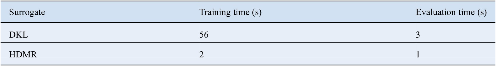
Table 6 compares plain GP regression using RBF and SM kernels, a stand-alone DNN, and DKL with RBF kernel, as well as HDMR with respect to RMSE for both NOx and soot emissions. We observe that the performance of DKL is significantly superior to the plain GPs with either the RBF or the spectral mixture kernel on both outputs. This is consistent with expectation, since, as discussed in Section 2.4, the 14-dimensional input space of our engine dataset would be expected to cause problems for plain GPs. DKL also outperforms a stand-alone DNN, indicating a genuine benefit in the combination of a GP and a DNN.
Table 6. Root mean squared error (RMSE) performance of the considered surrogates on the diesel dataset.
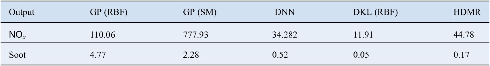
Abbreviations: DKL, deep kernel learning; DNN, deep neural network; GP, Gaussian process; HDMR, high-dimensional model representation.
In Figure 7, we show the RMSE loss history of the NOx regression for DKL and plain neural network during the training process. We observe that the prediction losses with respect to the experimental values of the DKL training throughout the training process is consistently lower than those of the plain DNN training. Even at the beginning of the training, it can be observed that the loss for the DKL prediction is lower than for the plain DNN prediction. This agrees with our expectation due to the existence of a GP at the end of DKL, which automatically computes the maximum a posteriori (MAP) estimate given the training dataset as the prediction. We can also see that the loss history curve for the DKL is much smoother than that for the DNN. Hence the RMSE loss of the DKL training process is a robust estimator for the performance of the trained model whereas for the DNN training, the RMSE estimates the performance of the model with larger uncertainty.
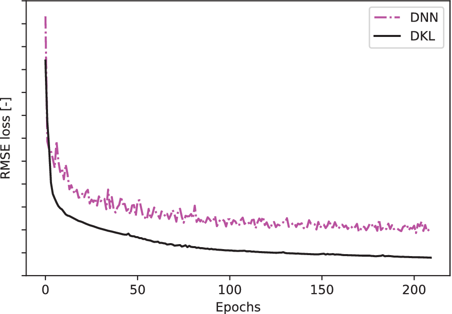
Figure 7. Loss history of training deep kernel learning (DKL) as well as a plain deep neural network (DNN) for  $ {\mathsf{NO}}_x $
regression.
$ {\mathsf{NO}}_x $
regression.
From Figures 5–7 and Table 6 we conclude that the DKL shows improvement over HDMR, plain GPs and plain neural networks in the regression tasks on the considered diesel engine emission dataset.
4. Conclusions
In this paper, we studied DKL as a surrogate model for diesel engine emission data. Instead of using a physical-based model for modeling the complex system, we have taken a purely data-driven approach. DKL was applied to a commercial Diesel engine dataset for NOx and soot emissions comprising 1,861 data points, with 14 operating condition variables as inputs. We employed a systematic two-stage procedure, consisting of a quasi-random global search and a local gradient-free optimization stage, to determine seven DKL hyperparameters, which include network architecture as well as kernel and learning parameters. It was found that the global search, conducted through sampling 1,000 Sobol points, was most effective in identifying a suitable set of hyperparameters. Local optimization was found largely ineffective for the network architecture hyperparameters, but led to minor improvement for the kernel and learning parameters. We compared DKL to standard deep feedforward neural networks, GPs, as well as HDMR, and the results indicate that, overall, DKL outperforms these methods in terms of regression accuracy as measured by RMSE on the considered 14-dimensional engine dataset for NOx and soot modeling. Further research themes could involve designing DKL with nonstationary kernel functions to deal with the heteroskedasticity of the input arguments.
Acknowledgments.
Changmin Yu is thankful to CMCL Innovations for the internship program offered.
Funding Statement
This work was partly funded by the National Research Foundation (NRF), Prime Minister’s Office, Singapore under its Campus for Research Excellence and Technological Enterprise (CREATE) program, and by the European Union Horizon 2020 Research and Innovation Program under grant agreement 646121. Changmin Yu was funded by a Shell PhD studentship. Markus Kraft gratefully acknowledges the support of the Alexander von Humboldt foundation.
Competing Interests.
The authors declare no competing interests exist.
Authorship Contributions
Conceptualization: M.S., S.M., M.K., and A.B.; Data curation: M.P., M.D., and V.P.; Formal analysis: C.Y., M.S., S.M., and G.B.; Funding acquisition: M.K., V.P., A.B., and S.M.; Investigation: C.Y., M.S., S.M., and G.B.; Methodology: M.S., S.M., and G.B.; Software: M.S., S.M., and G.B.; Supervision: S.M., M.K., V.P., and A.B.; Validation: S.M., G.B., M.P., and M.D.; Visualization: C.Y., M.S., and S.M.; Writing-original draft: C.Y., M.S., and S.M.; Writing-review & editing: S.M.; All authors approved the final submitted draft.
Data Availability Statement
The data used in this work are proprietary and confidential.
Ethical Standards
The research meets all ethical guidelines, including adherence to the legal requirements of the study country.


 Open access
Comments
No Comments have been published for this article.