


Impact Statement
Pipeline transport of slurries is an applied field wherein decision-making is driven by guidelines, rules-of-thumb and models derived from fundamental fluid mechanics. We demonstrate how ultrasound imaging can complement measurements of integral quantities, offering an avenue to reassess our fundamental understanding of established applied processes. We advocate for slowly settling slurries to gain mainstream recognition, next to the present dichotomy of settling and non-settling ones. This is related to the settling of conventionally non-settling slurries over long distances/times, foreshadowing shutdown. Similarly, laminar-to-turbulent transition is often boiled down to a critical velocity, touted as the most efficient operating point. Targeting this critical velocity via self-equilibrating behaviour is demonstrated while starting up a pipe. Particles initially in the bed are slowly entrained into the flow. The final stage involves an equilibrium, with all particles suspended and the flow having visible intermittency. This can serve as an alternative approach for starting up a pipeline.
1. Introduction
Pipeline transport of slurries is a matured field (Reference PatersonPaterson, 2012; Reference Thomas and CowperThomas & Cowper, 2017; Reference WaspWasp, 1983) where solids (‘payload’) are transported in a carrier liquid (‘vehicle’). Owing to the intrinsic breadth of slurry flows, distinctions are made to allocate slurries to categories. A major classification factor is whether the slurry is settling or non-settling, depending on the settling tendency of the particles. Accordingly, the slurry is treated as either pseudo-homogeneous (non-settling) or heterogeneous (settling). Commonly, classification is based on particle size, a typical threshold being 40  $\mathrm {\mu }$m. For non-settling slurries, varying the volume fraction of the particles additionally influences the rheology. Non-settling slurries offer a convenient avenue for simplification, with the option to model the two-phase system as an effectively single-phase, homogeneous, non-Newtonian fluid.
Even though flows of Newtonian fluids are almost always turbulent in practice, slurry flows can be laminar due to the significantly enhanced effective viscosity caused by the presence of particles. A key benchmark of a slurry pipeline (for a non-settling slurry) is the critical velocity at which the laminar–turbulent transition occurs. This serves two major roles: (1) to determine an appropriate model to predict total pressure drops and (2) to establish an operation point where the specific energy consumption (energy imparted to the slurry divided by the product of pipeline length and dry solids throughput) is minimized (Reference Pullum, Boger and SofraPullum, Boger, & Sofra, 2018). The latter aspect is relevant economically. For a non-settling slurry, the most favourable operation point would be just below the critical velocity. In contrast, for a settling slurry, it would be just above the critical velocity, so that turbulence would counter settling (Reference Wilson, Addie, Sellgren and CliftWilson, Addie, Sellgren, & Clift, 2006). From Newtonian fluid mechanics, transition is known to occur over a range of velocities and is accompanied by rich phenomena (Reference BarkleyBarkley, 2016). However, the slurry community typically reduce transition to a single point. This might be driven by pragmatism, since only pressure gradients are needed to design pipelines (Reference Güzel, Burghelea, Frigaard and MartinezGüzel, Burghelea, Frigaard, & Martinez, 2009). Furthermore, a minimum allowable transport velocity is determined by applying a safety margin to the critical velocity (Reference Javadi, Pirouz and SlatterJavadi, Pirouz, & Slatter, 2020).
While slurry flows in pipelines have been studied extensively, experimental work for the laminar–turbulent transition in non-settling slurries is often restricted to time-averaged pressure drop measurements. Occasionally, pressure fluctuations (standard deviation or time series) are also used to detect the laminar–turbulent transition (Reference El-Nahhas, El-Hak, Rayan, Vlasak and El-SawafEl-Nahhas, El-Hak, Rayan, Vlasak, & El-Sawaf, 2004; Reference SlatterSlatter, 2005; Reference Vlasak and CharaVlasak & Chara, 2004). Only a handful of studies consider local features of the flow using ultrasonic techniques (Reference Benslimane, Bekkour, François and BechirBenslimane, Bekkour, François, & Bechir, 2016; Reference Thota Radhakrishnan, Poelma, van Lier and ClemensThota Radhakrishnan, Poelma, van Lier, & Clemens, 2021).
We take a close look at the laminar–turbulent transition of a common model slurry, a kaolin–water mixture (21 % w/w or 9 % v/v). Based on rules-of-thumb, this slurry is non-settling (median size  $= 5.18~\mathrm {\mu }$m, measured settling velocity $= 342$ nm s $^{-1}$). It flows in a pipe loop with an inner diameter of 0.1 m, generally considered as a lower threshold for industrial-scale pipelines (Reference Pullum, Boger and SofraPullum et al., 2018). This slurry is dense enough to possess non-Newtonian properties (yield-pseudoplastic fluid). The flow is probed with time-averaged pressure drop measurements as well as ultrasound imaging. Using cross-correlation techniques, ultrasound imaging velocimetry (UIV) returns velocity profiles (Reference PoelmaPoelma, 2017). The ultrasound image intensities furthermore reveal the spatial distribution of the solids in the slurry. Typically, brighter intensities suggest more particles. However, one must be aware of the role of attenuation, which leads to reduced intensities away from the transducer. We perform experiments with two trajectories: one wherein the flow velocity is increased in time (system not homogenized prior to setting desired flow conditions) and another wherein the flow velocity is reduced in time (system homogenized prior to setting desired flow conditions). We aim to illustrate two types of long-time-scale transients, which are dependent on the experimental trajectory. The usage of long measurement times in an industrial-scale facility and ultrasound imaging help unearth and explain observations which would have otherwise been missed. Knowledge of these transients could be relevant when operating pipelines close to the favourable point of the laminar–turbulent transition.
In § 2, we describe the experimental facility and the various experiments considered. Two types of experiments are performed: ‘unaltered inflow’ (§ 3) and ‘ramped inflow’ (§ 4). From these experiments, two types of transient behaviours are captured, which we refer to as ‘slowly settling’ (§ 5) and ‘self-equilibration’ (§ 6). The key conclusions are summarized in § 7.
2. Experimental set-up and procedures
The experiments are performed in a facility specifically designed for slurry flows (‘ $\beta$-loop’, Deltares, Delft, The Netherlands), a schematic of which is shown in figure 1. The facility contains more than 4 m $^{3}$ of slurry. A slurry reservoir contains the bulk of the slurry. The pipes are made of polyvinyl chloride with an internal diameter of $D = 10$ cm. The flow is driven by a variable frequency centrifugal slurry pump (NT 3153, Xylem). The pump frequency can be controlled manually up to a maximum of 50 Hz. Three valves in the facility (bypass valve and two valves to pipe) can be regulated manually to alter the flow. The volumetric flow rate is monitored by an electromagnetic flow meter (Optiflux 2300C, Krohne). Submersible pressure transducers (PDCR5031, GE) and temperature sensors (STS-PT100, Ametek) are installed at several locations to measure the absolute pressure and temperature, respectively. Pressures, temperatures and the volumetric flow rate are logged at 50 Hz over a working day ( $\sim$8 hours).

Figure 1. Schematic of the experimental facility and the region of interest (not to scale).
Ultrasound images were recorded using a SonixTOUCH Research (Ultrasonix/BK Ultrasound) coupled to a linear array transducer (L14-5/38). While setting up an ultrasound imaging measurement, a balance needs to be struck between imaging frame rate, field of view and line density (see Chapter 14 in Reference Bushberg, Seibert, Leidholt and BooneBushberg, Seibert, Leidholt, & Boone, 2012). In our experiments, we achieve imaging depths of 6 cm, and an imaging rate of 287 frames per second by reducing the sector to 50 % and line density to 64. The imaging resolutions in the axial direction (direction parallel to beam propagation) and lateral direction (direction perpendicular to beam propagation) are 0.6 and 0.3 mm, respectively. Velocity results were generated using PIVware (Matlab script based on Reference WesterweelWesterweel (1993)) followed by sweep correction (Reference Zhou, Fraser, Poelma, Mari, Eckersley, Weinberg and TangZhou et al., 2013). Further technical details surrounding ultrasound imaging (velocimetry) measurements and the corresponding post-processing can be found in §§ 3.2 and 3.3 of Reference Dash, Hogendoorn, Oldenziel and PoelmaDash, Hogendoorn, Oldenziel, and Poelma (2022). The axial spatial resolution of the velocimetry measurements is 0.6 mm while the temporal resolution is 182 ms. The performance of ultrasound imaging (velocimetry) in particle-laden flows is reduced due to attenuation. In several of the results presented herein, it is evident that the quality of the velocimetry results is inferior farther away from the ultrasound transducer.
For a detailed overview of the slurry characterization, the interested reader is directed to the supplementary material available at https://doi.org/10.1017/flo.2022.18. Only a short summary is provided here. In brief, the slurry has a mass density of  $\rho = 1152.1$ kg m $^{-3}$ and contains fine particles with a median size of 5.18 $\mathrm {\mu }$m. Its non-Newtonian behaviour can be characterized by the Herschel–Bulkley model ( $\tau = \tau _y + K\dot {\gamma }^n$), whose parameters are determined via a rheogram between the shear stress, $\tau$, and the shear rate, $\dot {\gamma }$. The slurry has a yield stress, $\tau _y =$ 0.8889 Pa, a consistency index, $K = 0.1579\ {\rm Pa}\,{\rm s}^{0.4579}$, and a behaviour index, $n = 0.4579$ at 18 $^{\circ }$C.
The slurry settles overnight ( $\sim$16 hours) during a prolonged period of shutdown, and the system is stratified (all particles in a stationary bed and clear liquid atop). Two types of experimental ‘trajectories’ are considered: one wherein the system is homogenized before setting the desired flow rate and another wherein the system is not homogenized. The two trajectories are denoted by $\downarrow$ and $\uparrow$, respectively, and symbolize the approach employed to arrive at the desired flow velocities. In both cases, prior to measurements, pressurized air is released at the bottom of the reservoir to resuspend the settled particles. Thereafter, a mixing pump suspended in the reservoir reduces particle settling. These actions are necessary for the reservoir and do not affect the pipe.
The  $\uparrow$ experiments require a certain degree of care. Even before resuspending the settled slurry in the reservoir, the valves to the pipe are slowly opened completely to equalize the pressure across it. This step needs to be done carefully, failing which the stationary bed may get disturbed. With the bypass valve completely open and the valves to the pipe completely closed, the slurry pump is turned on at a frequency of 20 Hz and the flow occurs exclusively in the bypass loop between the reservoir and the bypass valve. Then, the bypass valve is closed gradually until the desired flow rate is achieved. Using the bypass valve, bulk velocities up to $U_b=1.48$ m s $^{-1}$ can be attained. To obtain even higher velocities, the pump frequency needs to be increased.
For the  $\downarrow$ experiments, the procedure requires less care. With the bypass valve completely open and the valves to the pipe completely closed, the slurry pump is turned on at a frequency of 20 Hz and the flow occurs exclusively in the bypass loop. The valves to the pipe are then fully opened and then the bypass valve is completely closed. The pump frequency is then increased to 50 Hz and a bulk velocity >3.5 m s $^{-1}$ is achieved. The system is maintained in this state for at least 30 minutes. To achieve a target volumetric flow rate $\geq$1.48 m s $^{-1}$, the pump frequency is lowered to an appropriate value. To achieve bulk velocities <1.48 m s $^{-1}$, the pump frequency is brought down to 20 Hz and the bypass valve is gradually opened until the desired volumetric flow rate is reached.
Two types of experiments (not to be confused with the two trajectories) are considered here. The first are experiments wherein the system settings (pump and valves) are left untouched once the desired flow rate has been achieved, until shutdown. The only time the system is perturbed is midway through the experiments while wall sampling (tapping a slurry sample from a port on the wall). This tap is present along the inner curvature of the 90 $^{\circ }$ bend, 5.5 pipe diameters downstream of it. The second set of experiments are experiments wherein the bulk velocity is either gradually increased ( $\uparrow$) from a fully stratified state, or decreased ( $\downarrow$) following homogenization at the highest flow rate, over the course of a working day. No wall sampling is performed here. These are referred to as ‘unaltered inflow’ and ‘ramped inflow’ experiments, respectively.
A total of nine ‘unaltered inflow’ experiments are considered: [1.87, 1.47, 1.46, 1.30, 1.15, 0.99, 0.80, 0.63] m s $^{-1} \downarrow$, 0.60 m s $^{-1} \uparrow$. The velocities in this list are the target bulk velocities and the pump/valves are left untouched once the conditions are achieved. Ultrasound images are recorded in the horizontal pipe section (top and side) as well, towards the end of the working day. The streamwise location on the horizontal pipe is 17 pipe diameters upstream of the bend and nearly 800 pipe diameters downstream of the entrance.
In contrast, four ‘ramped inflow’ experiments are performed with a combination of the two trajectories ( $\uparrow$ and $\downarrow$) and two ultrasound imaging locations (top and ‘bottom’). Underneath the horizontal pipe lie support structures preventing us from achieving a normal contact angle between the pipe and the ultrasound transducer. Thus, the ‘bottom’ measurements must be inferred in a semi-quantitative manner. Decisions to alter the flow rate had to be made on the fly depending on what was observed in real time, given the constraint of the working day. Since the facility is not computer-controlled, the rate of ramping is arbitrary. By observing the trends in measured pressure drops and ultrasound images, as well as time remaining in the day, decisions to alter the flow conditions were made. Since flow rates are altered manually and arbitrarily, it would be difficult to reproduce the experiments in a one-to-one manner. The aim of these experiments was to have a close look at the laminar–turbulent transition in this flow loop.
3. Results: unaltered inflow experiments
3.1 Global characteristics: pressure drop and bulk velocity
The volumetric flow rates and pressure drops in the horizontal pipe section measured during the unaltered inflow experiments for several initial settings are shown in figure 2(a,b), wherein each time series is normalized with its initial value. After the desired initial condition was attained (time = 0 minutes), the pump/valves were left untouched until shutdown (sharp decreases in bulk velocity or pressure drop). Since each experiment in this measurement campaign lasted over a working day, it allowed us to record global system behaviour over the course of several hours.

Figure 2. (a) Bulk velocity and (b) pressure drop in the horizontal pipe section for different initial conditions. Normalization is performed with corresponding value at 0 min. Each experimental dataset is vertically offset by 0.1 in both panels. The black lines denote the moments when wall sampling was performed. (c) Corresponding pipe rheograms. The black circles correspond to experiments wherein no remarkable transient behaviour is observed, whereas for the other experiments, the transient behaviour is shown with the corresponding colourbar (left and right for 0.63 m s $^{-1} \downarrow$ and 0.60 m s $^{-1} \uparrow$, respectively). The curved arrow represents the trajectory of the wall shear stress for 0.60 m s $^{-1} \uparrow$. The analytical solution for laminar flow holds true for Herschel–Bulkley rheology, and the equation is reproduced in the supplementary material.
When the initial bulk velocity is high ( ${\geq} 0.99$ m s $^{-1}$), the bulk velocity as well as the pressure drop remain steady and fairly constant over the entire day (fluctuations within 2 %). For the example of 0.80 m s $^{-1} \downarrow$, there are visible long-time-scale fluctuations in the bulk velocity, the causes for which are unclear. The two most interesting examples are 0.63 m s $^{-1} \downarrow$ and 0.60 m s $^{-1} \uparrow$, whose behaviours are peculiar.
For 0.63 m s $^{-1} \downarrow$, the bulk velocity drops by 20 % over 6.5 hours, while the pressure drop in the system rises by 30 %. This is detrimental from a practical perspective. Were these trends to continue, a complete shutdown could occur, and no particles would get transported. This observation already hints that some form of settling is present in the system despite the slurry being ‘non-settling’, which will be verified later in § 5. Settling of particles would result in the formation of a stationary bed, leading to an increased resistance (higher pressure drop), which causes a reduction in the flow rate. The reduced flow rate then further facilitates particle settling allowing this transient to sustain.
At the other end of the spectrum lies the example of 0.60 m s $^{-1} \uparrow$. Basically, the bulk velocity rises by 50 % over 4 hours after which it attains some form of equilibrium. Based on the above example of 0.63 m s $^{-1} \downarrow$ where we suspect the presence of settling, the most obvious ansatz would be that there is gradual erosion of the bed accompanied by particle resuspension in 0.60 m s $^{-1} \uparrow$. This ansatz is verified later in § 6. Resuspension of particles would lead to an increased cross-sectional area, which would reduce resistance to the flow leading to an increased flow rate. The increased flow rate would trigger further resuspension. In the initial phase wherein the bulk velocity rises gradually, the pressure drop varies mildly. When there is a transition from a transient state to a steady state, there is a sharp rise in the pressure drop with the peak reaching as high as 30 %. However, during the steady-state phase, we see that the pressure drop reduces gradually by 10 % over the course of 4 hours.
One caveat in the observations for 0.60 m s $^{-1} \uparrow$ is that the causality behind equilibration might be influenced by wall sampling. From figure 2(a,b), it is evident that wall sampling for 0.60 m s $^{-1} \uparrow$ is immediately followed by a jump in the pressure drop and volumetric flow rate. This is in contrast to all the other $\downarrow$ experiments, where wall sampling has no visible effect. In this scenario, we suspect that the equilibration process is triggered by an external perturbation rather than it being an intrinsic phenomenon. We conjecture how wall sampling may have influenced the flow in the $\uparrow$ experiments. The slurry loop is a pressurized system and the internal pressure near the wall sampling location is higher than atmospheric pressure. When the tap is opened, this location is suddenly exposed to lower, atmospheric pressure. This leads to an increased pressure drop between the horizontal pipe and the wall sampling location, which would increase the bulk velocity in the system. If the system is already homogeneous and well mixed (like in $\downarrow$ experiments), the increased velocity should not affect the distribution of particles. However, if particles are settled (like in $\uparrow$ experiments), the increased velocity would resuspend them and possibly homogenize the slurry. This might explain why wall sampling seemingly influences the $\uparrow$ experiments but not the $\downarrow$ experiments. The seemingly benign action of wall sampling appears to be more complicated and one must be aware of its potential implications.
In figure 2(c), the corresponding pipe rheograms (wall shear stress versus pseudo shear rate ( ${=} 8U_b/D$)) are shown. To define the pseudo shear rate, the bulk velocity, $U_b$, and the pipe diameter, $D$, are required. We report pipe rheograms rather than Moody diagrams (skin friction factor versus Reynolds number) to avoid dealing with the selection of a model to define the Reynolds number for a non-Newtonian slurry. For experiments with relatively steady-state conditions, the laminar–turbulent transition can be clearly seen. The analytical solution under laminar conditions is based on (9) in Reference van den Heever, Sutherland and Haldenwangvan den Heever, Sutherland, and Haldenwang (2014). The pipe rheogram undergoes a gradual transition from laminar to turbulent conditions, typical of non-Newtonian fluids/slurries (unlike Newtonian fluids that show an abrupt transition). Based on this plot, one could conclude that 0.80 m s $^{-1} \downarrow$ has laminar conditions, while the remaining points are non-laminar. We later show via the results of the ‘ramped inflow’ experiments that the critical velocity for the present combination of the slurry and flow facility is between 0.85 and 0.89 m s $^{-1}$. The overlapping results of 1.47 m s $^{-1} \downarrow$ and 1.46 m s $^{-1} \downarrow$ (performed 12 days apart) suggest that experiments are repeatable in the turbulent regime.
For the plots demonstrating transient behaviour, a moving mean over 10 s is applied, and thereafter only data points at every 2 s are shown. For 0.63 m s $^{-1} \downarrow$, the initial condition agrees with the analytical solution for laminar flows. However, with increasing time, the wall shear stresses exceed the analytically expected value for a homogeneous system, suggesting loss of homogeneity. On the other hand, for 0.60 m s $^{-1} \uparrow$, the measured wall shear stress is initially slightly higher than the analytical solution, possibly due to the presence of a bed. With increasing time, the agreement with the analytical solution improves, before sharply deviating from the analytical solution. After reaching a maximal deviation from the analytical solution (denoted by curved arrow in figure 2c), the wall shear stress slowly arrives at a value close to the measurement of 0.99 m s $^{-1} \downarrow$. As a whole, the pipe rheogram appears to have a minimum, which is commonplace for settling slurries. This example shows that despite similar initial conditions in the volumetric flow rate, the end result could vary greatly depending on the initial conditions of the slurry homogeneity.
Seldom are pipe rheograms presented in this manner where the transient behaviour is evident. Observing these transients requires periods of several hours. Typically, measurements are presented in a manner which reflect that all measurements are performed at steady state. This is especially true for slurries that are classified as non-settling. The results herein suggest that time can become a relevant factor in hydraulic design, especially when considering conventionally non-settling slurries in a large or long pipe. Studies in smaller pipes (laboratory scale) might miss this behaviour altogether as higher flow velocities compensate for the smaller diameters to achieve similar Reynolds numbers (thus, increased chance for particles to be resuspended).
3.2 Local characteristics: velocity profiles
Any deviation from homogeneity in the slurry mixture should affect the otherwise axisymmetric time-averaged velocity profiles in the horizontal pipe section. For this purpose, we present the time-averaged velocity plots from UIV in figure 3(a). For each example, two plots are shown – one wherein images were taken from the top and another from the side. The overlap of the two velocity profiles, or lack thereof, can already serve as an indicator of homogeneity in the system. All these measurements were performed within 30 minutes prior to shutdown and are based on a total of 43.6 s (five discontinuous datasets spanning 8.72 s). At locations with low signal-to-noise ratio (as defined in Reference Dash, Hogendoorn, Oldenziel and PoelmaDash et al. (2022)), the velocity data are excluded. Data quality is typically low very close to the wall (due to high velocity gradients) and far away from the wall (due to attenuation of ultrasound waves).
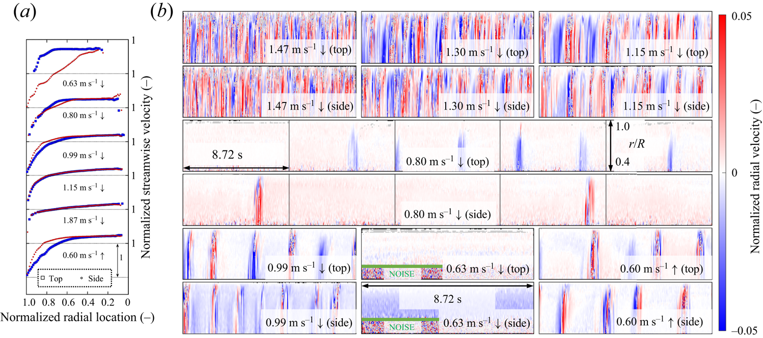
Figure 3. (a) Presence/absence of symmetry in time-averaged velocity profiles. (b) Spatio-temporal plots of radial velocity normalized by bulk velocity. At the time of measurement, for 0.63 m s $^{-1} \downarrow$, $U_b =$ 0.51 m s $^{-1}$ while for 0.60 m s $^{-1} \uparrow$, $U_b =$ 0.92 m s $^{-1}$. The measurements from top and side are not simultaneous. The horizontal extent of each box is 8.72 s. The results of 0.63 m s $^{-1}$ $\downarrow$ are afflicted by noise away from the wall (underneath the green line) and should not be mistaken for turbulence.
For [1.87, 1.15] m s $^{-1} \downarrow$, the two velocity profiles overlap well, implying that the system should be homogeneous. Similar overlap also holds true for [1.47, 1.46, 1.30] m s $^{-1} \downarrow$ (data not shown). With decreasing bulk velocity, the region near the wall with a high velocity gradient becomes larger, resulting in a less flat velocity profile. For 0.99 m s $^{-1} \downarrow$ and 0.80 m s $^{-1} \downarrow$, the loss of axisymmetry is visible but not severe. However, for the two peculiar cases, 0.63 m s $^{-1} \downarrow$ and 0.60 m s $^{-1} \uparrow$, the deviations from axisymmetry are much more emphatic – the velocity profiles measured from the top and side show poor overlap.
At least for 0.63 m s $^{-1} \downarrow$ where a stationary bed is expected to be present, the velocity profile from the top is expected to possess more momentum. Thus the loss of axisymmetry for 0.63 m s $^{-1} \downarrow$ is not too surprising. For the 0.60 m s $^{-1} \uparrow$ experiment (where 0.60 m s $^{-1}$ is the initial velocity), the bulk velocity was already 0.92 m s $^{-1}$ by the time the ultrasound images were recorded. However, the deviation from axisymmetry is much stronger than for either 0.80 m s $^{-1} \downarrow$ or 0.99 m s $^{-1} \downarrow$. This observation, together with the example of the gradually dropping pressure gradient in figure 2(b), might suggest that the homogenization process is perhaps incomplete.
Our velocity measurements imply that modelling two-phase fine-grained slurry flows as a homogeneous, effectively single-phase, non-Newtonian liquid under non-turbulent conditions must be done at one's peril. The additional possibility of inhomogeneity must not be neglected. Thus, it would be far-fetched for us to directly associate our observations in the transitional regime with those in homogeneous systems. It is well known that in such homogeneous non-Newtonian systems, the time-averaged velocity profiles in the transitional regime are non-axisymmetric, unlike the laminar or the turbulent regime (Reference Escudier, Poole, Presti, Dales, Nouar, Desaubry, Graham and PullumEscudier et al., 2005; Reference Escudier and PrestiEscudier & Presti, 1996; Reference Güzel, Burghelea, Frigaard and MartinezGüzel et al., 2009; Reference Peixinho, Nouar, Desaubry and ThéronPeixinho, Nouar, Desaubry, & Théron, 2005; Reference Wen, Poole, Willis and DennisWen, Poole, Willis, & Dennis, 2017).
To have a closer look at the flow topology, instantaneous velocities are considered next. In figure 3(b), spatio-temporal radial velocity profiles for seven of the nine experiments are shown. Basically, instantaneous radial velocity profiles are stacked together. To estimate the length of the structures, the temporal axis can be converted to a spatial axis using the bulk velocity. For 1.87 m s $^{-1} \downarrow$, capturing the instantaneous velocities becomes challenging due to the high velocities in the flow. The experiments of 1.46 m s $^{-1} \downarrow$ were a repeatability test for 1.47 m s $^{-1} \downarrow$, and hence are not presented.
For 1.47 m s $^{-1} \downarrow$, 1.30 m s $^{-1} \downarrow$ and 1.15 m s $^{-1} \downarrow$, the entire spatio-temporal plot is filled with fluctuations, and thus can be classified as turbulent. This is not unexpected based on the pipe rheogram in figure 2(c). As a result, the system is well mixed and explains why the corresponding time-averaged velocity profiles are symmetric. For 0.63 m s $^{-1} \downarrow$, the flow topology is laminar at the time of measurement. It seems that the velocimetry results for 0.63 m s $^{-1}$ $\downarrow$ are corrupted away from the wall, due to the domination of noise. We believe this is caused by ultrasonic attenuation which itself is a function of spatial particle distribution. Velocity results underneath the green line are unreliable. For the remaining cases of 0.99 m s $^{-1} \downarrow$, 0.80 m s $^{-1} \downarrow$ and 0.60 m s $^{-1} \uparrow$, the flow topology can be classified as intermittent or transitional. Of course, for 0.60 m s $^{-1} \uparrow$, the bulk velocity had risen significantly to 0.92 m s $^{-1}$ by the time these measurements were performed. Of the three intermittent cases, that of 0.80 m s $^{-1} \downarrow$ has the sparsest levels of intermittency. Across all the examples, the root mean square of the radial velocity fluctuations is approximately 2 %–3 % of the bulk velocity, meaning that they are typically $> 0.02$ m s $^{-1}$ (several orders of magnitude higher than the measured settling velocity of 342 nm s $^{-1}$). While we only present the radial velocity profiles here, the passage of these intermittent structures also affects the corresponding streamwise velocity profiles. Since ultrasound images are recorded at arbitrary times, the time-averaged velocity profiles from top and side might differ, depending on the degree of intermittency present when the ultrasound images were recorded.
The combined insights from the global point of view (pipe rheogram) and the local point of view (spatio-temporal distribution of velocities) can help one classify the flow regime. In the slurry community, especially for pipes, there exists a dichotomy in the flow regimes – a laminar and a turbulent regime separated by a single critical velocity. This critical velocity for transition is the point at which the wall shear stress begins to deviate from the analytical solution for laminar flows. Our results show that the process has a lot more intricacies. The example of 0.80 m s $^{-1} \downarrow$ is sparsely intermittent but the corresponding wall shear stress lies on the analytical solution for laminar flows. The case of 0.99 m s $^{-1} \downarrow$ as well as the final state of 0.60 m s $^{-1} \uparrow$ (0.92 m s $^{-1}$) deviate visibly from the laminar solution and could possibly be considered as approximate critical velocities from the perspective of slurry system design. As explained in § 1, operating the pipeline close to the laminar–turbulent transition is considered most favourable. However, even if sparse levels of intermittency are present at velocities lower than the conventional critical velocity, it might be an even more favourable operating point. Thus, it might be valuable to consider a range of transitional velocities instead of reducing it to a point.
While flows of slurries in pipes are broadly categorized into two regimes, transitional flows in open-channel flows are recognized as a regime rather than an intermediate step. For example, Reference HaldenwangHaldenwang (2003) achieves this by distinguishing between the onset of transition and the onset of full turbulence. Reference Baas, Best, Peakall and WangBaas, Best, Peakall, and Wang (2009) use ultrasonic velocity profiling to extract time-averaged and time-resolved velocities, and identify five different flow regimes: turbulent flow, turbulence-enhanced transitional flow, lower and upper transitional flow, and quasi-laminar plug flow. This is not to say that the slurry community is unfamiliar with the concept of intermittent flows in pipes. However, slurry flows in pipes could benefit from a more refined classification of the flow regimes.
4. Results: ramped inflow experiments
Four day-long ramped inflow experiments were performed, wherein two types of trajectories were followed: ramp-up ( $\uparrow$) and ramp-down ( $\downarrow$). Shown in figure 4 are the pipe rheograms for both experimental trajectories. At lower pseudo shear rates (conversely, lower bulk velocities), the flow typically displays transient behaviour irrespective of the experimental trajectory (see the two examples that are shown enlarged in figure 4a). In a few instances, the transient behaviour is not as evident. However, our observations are limited to the time spent at each measurement point. At higher pseudo shear rates, the flow rates were altered after a few minutes (typically ranging between 3 and 10 minutes). At lower pseudo shear rates, where transient behaviour was evident, the observation times were long enough to capture transient behaviour but short enough so that the the entire range of velocities could be traversed across the working day.

Figure 4. Pipe rheograms for the ramped inflow experiments. The four datasets are shown (a) with and (b) without an offset. The identifiers ‘top’ and ‘bottom’ refer to the location of ultrasound imaging and are unrelated to the pressure drop measurements. Measurements wherein no transient behaviour was seen are plotted as triangular markers. Colour of the circular markers indicates the time passed since the flow rate had been set. In (b), a few relations popular in the slurry community are also plotted. ‘Laminar flow’: analytical solution for a laminar, pipe flow of a Herschel–Bulkley fluid. ‘Turbulent flow (WT)’: turbulent flow model of Reference Wilson and ThomasWilson and Thomas (1985) and Reference Thomas and WilsonThomas and Wilson (1987). ‘Turbulent flow (S)’: turbulent flow model of Reference SlatterSlatter (1995). Equations for these relations are reproduced in the supplementary material. The inset in (b) zooms in on the beginning/end of observed steady-state behaviour.
From the global behaviour of the pipe rheograms in figure 4(b), a few things can be clearly deduced. Under laminar conditions (transient behaviour), the measured wall shear stress slightly exceeds the analytically expected value. As the flow approaches the point of transition (when experimental data begin deviating from the analytical solution for laminar flows), the agreement between the experimental data and the analytical solution improves. This might be caused by the improved homogeneity in the system, as the analytical solution does not account for inhomogeneities.
There are a couple of subtle differences with respect to the pipe rheogram in figure 2(c). In figure 2(c), the results of 0.63 m s $^{-1} \downarrow$ deviate strongly from the laminar solution, as compared with the ramp-down results in figure 4. One possible explanation for this is that in the ramped inflow experiments, the system is perturbed at irregular intervals by adjusting the bypass valve to attain a new flow rate. Another difference is related to how the ramp-up results differ from those of the unaltered inflow experiment of 0.60 m s $^{-1} \uparrow$. For 0.60 m s $^{-1} \uparrow$, the wall shear stress showed a small abrupt deviation from the laminar solution before gradually arriving closer to the trendline for non-laminar flows (see inset of figure 2c). No such abrupt deviation is visible in the ramp-up experiments. This might provide further weight to the argument that the equilibration in that particular unaltered inflow experiment was indeed triggered by wall sampling.
In the slurry community, numerous criteria to detect the laminar–turbulent transition point have been developed (Reference Eshtiaghi, Markis and SlatterEshtiaghi, Markis, & Slatter, 2012). One of the simplest ways to determine a transitional velocity is by the so called intersection method, first used by Reference HedströmHedström (1952). Basically, a turbulent flow model needs to be selected, and its intersection with the analytical solution for laminar flow is considered to be the transitional velocity. According to the measurements, the transitional velocity is determined to lie between 0.85 and 0.89 m s $^{-1}$. In the present case, selecting the model of Reference Wilson and ThomasWilson and Thomas (1985) (0.90 m s $^{-1}$) for the intersection method works better than selecting the model of Reference SlatterSlatter (1995) (1.03 m s $^{-1}$). Finally, in the turbulent regime, the Slatter model performs better in predicting the wall shear stress. This also serves as a cautionary tale on directly using various models. While these models are capable of providing a ballpark for pressure gradients or critical velocities, they need not necessarily work perfectly. For example, the models might be sensitive to the choice of the fitted parameters characterizing the rheology (Reference Vlasak and CharaVlasak & Chara, 1999).
Based on relatively well-overlapping curves in figure 4(b), one might conclude that there are no hysteresis effects in the system (since data points collapse on one another irrespective of the protocol). However, this is not strictly true. In the inset of figure 4(b), it can be seen that the pseudo shear rates below which transient effects are evident for the ramp-up experiments are higher than for ramp-down experiments. For clarity, only the non-transient data are shown in the inset of figure 4(b), to highlight that the onset occurs at different pseudo shear rate. We identify these two critical pseudo shear rates (or velocities) as suspending velocity (ramp-up) and deposit velocity (ramp-down). The former is the critical velocity above which all particles are suspended, whereas the latter is the critical velocity below which particles begin to deposit. These concepts are well established in the context of settling slurries (Reference Carleson, Drown, Hart and PetersonCarleson, Drown, Hart, & Peterson, 1987). In our experiments, the suspending velocity exceeds the deposit velocity, subtly illustrating the presence of hysteresis.
5. Slowly settling behaviour
While discussing the unaltered inflow experiments, it was shown that if the system was homogenized at a very high velocity and then the flow rate was reduced to a desired value, a steady flow rate could be obtained under intermittent/turbulent conditions. However, under laminar conditions, the flow rate dropped continuously and gradually, while the pressure gradient rose. Spatio-temporal plots of ultrasound image intensities recorded from top, in figure 5(a), show that the intensities are lower under laminar than turbulent conditions proving that the slurry is not homogenized under laminar conditions. All of this led us to hypothesize that this supposedly ‘non-settling’ slurry experiences settling.

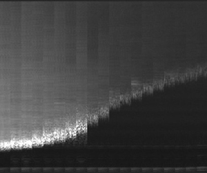
Figure 5. (a) Spatio-temporal evolution of ultrasound image intensities under laminar and turbulent conditions (ramp-down experiments), when viewed from top. (b) Measured volumetric flow rate. (c) Formation of stationary bed as imaged from bottom. Results in (b) and (c) are simultaneous.
To verify this hypothesis, a separate experiment was performed. After operating the system at a relatively high velocity (albeit much lower than the maximum velocity), the flow rate was reduced to a value in the laminar regime. We capture ultrasound images from the bottom of the pipe. We concurrently record the flow meter readings, from which the bulk velocity can be determined. As expected, we observe a gradual decline in the measured bulk velocity as shown in figure 5(b). However, the rate of decline (0.8 mm s $^{-1}$ per minute) is higher than in figure 2(a) for 0.63 m s $^{-1} \downarrow$ (0.3 mm s $^{-1}$ per minute). This suggests that the transient behaviour is sensitive to the initial conditions.
The simultaneously recorded ultrasound images verify our hypothesis regarding the settling of particles and the formation of a stationary bed. This is shown in figure 5(c), wherein the thickness of the stationary bed grows in time. Since the static background is subtracted from the images, the pipe wall and the stationary bed appear dark in figure 5(c). Next to it is a thin, bright patch which we identify as mobile bed layer. Beyond that is the slurry which is still suspended. The effect of the growing stationary bed height is also visible on the intensity of the images. As the bed gets thicker with time, the attenuation of the ultrasonic waves grows. As a result, the image intensity of the sliding bed and the suspended slurry reduces. We can claim that the gradual reduction in measured volumetric flow rates is correlated to the settling of particles leading to a bed formation. These observations seemingly contradict common rules-of-thumb wherein such fine-grained kaolin slurries are assumed to be non-settling.
Reference Clarke and CharlesClarke and Charles (1997) also observed a slow accumulation of a stationary deposit, leading to a gradual reduction in flow rate (albeit for a slightly coarser kaolin slurry). In this context, we agree with Reference Clarke and CharlesClarke and Charles (1997) in their statement ‘While many slurries may be classified as either settling or non-settling, it is sometimes difficult to assign a slurry to one of these categories, and thus it is more appropriate to classify it as “slowly-settling”’. Such a classification is yet to be acknowledged in mainstream literature. This is not to say that the slurry community is unfamiliar with this behaviour. Reference ThomasThomas (1961) has stated that the critical deposit velocity (the velocity below which a stationary bed forms) coincides with the transition from laminar to turbulent flow. While not shown, we do not observe any bed formation under turbulent flow conditions, in line with Reference ThomasThomas (1961). Reference Javadi, Pirouz and SlatterJavadi et al. (2020) write ‘for slow settling materials…the laminar regime transportation can be adopted for relatively short distances since the likelihood of a density profile formation is expected to be relatively low’. Subsequently, the authors also write about a maximum pipeline length which can be accepted, before blockage becomes an issue under laminar conditions. Similarly, Reference Thomas, Pullum and WilsonThomas, Pullum, and Wilson (2004) write ‘There are a number of long distance slurry pipelines that have transported fine particle slurries under laminar flow conditions… [Reference Aude, Derammelaere and WaspAude et al. (1996)]…concluded that even fine particles settled slowly towards the bottom of the pipe under laminar flow conditions, although this might not occur for the first few kilometers of travel’. The results presented here should not be confused with stabilised laminar slurry flow, Stab-flo(w). Stab-flo(w) involves transporting coarse particles in a suspension of carrier liquid and fine particles. The idea is that the fine particles introduce a yield stress, which would prevent settling of the coarse particles. All of this allows transporting the slurry under laminar conditions (more energy efficient) while maintaining stability (lack of settling). Nonetheless, several works have identified that Stab-flo(w) conditions are not as stable and settling of the coarse particles does occur. See Reference Thomas, Pullum and WilsonThomas et al. (2004) and Reference PatersonPaterson (2012) for detailed overviews. In any case, the settling that is observed in our experiments is that of fine particles themselves, which might also be of relevance for Stab-flo(w).
Experiments similar to those considered here (measuring global and local quantities) can be used to establish critical pipe lengths for which transport of slurries under laminar conditions can be executed without the danger of blockage (for example, by performing experiments in pipes of various lengths). This would also allow one to adjudge whether a pipeline transporting fines should be operated on the laminar side of the laminar–turbulent transition, which is considered to be more efficient. While practitioners may be familiar with slow settling, its obscurity in academic literature prevents the possibility for it to be thoroughly analysed to formulate/reassess guidelines.
6. Self-equilibrating behaviour
In this section, we take a closer look at the self-equilibrating behaviour. Such behaviour was evident in the two ramp-up experiments (ramped inflow experiments wherein the system is not initially homogenized; in one experiment ultrasound images are recorded from the top, and from the ‘bottom’ in the other), whose results are reported here. Figure 6 compiles the key results from the ramp-up experiments. Note that only results concerning the self-equilibration phenomenon from these measurement days are shown. These events span about 100 minutes, which is a fraction of the working day.

Figure 6. (a) Temporal evolution of bulk velocity during the self-equilibrating process on two separate days. The markers indicate moments at which ultrasound images were recorded. There are 64 markers in the left panel and 48 in the right panel. Coloured patches correspond to one setting of the slurry pump frequency and bypass valve opening fraction. (b) Corresponding temporal evolution of pressure gradient. (c) Spatio-temporal features of the flow corresponding to the patches and markers in (a). The numbering in the panels gives an indication of how these panels are related to the markers in (a). All measurements based on 8.72 s. (d) Spatio-temporal features of the image intensity. Extents of axes same as (c). The plot of T4–T3 shows that the process of homogenization is incomplete at T3.
In figure 6(a), we show the evolution of the bulk velocity in time on two separate days of ramp-up experiments. Sudden jumps in the bulk velocity indicate that the flow rate was altered manually (for example, far right side of the top-left blue panel). In the ramp-up experiment wherein imaging was performed from the top, we observe a period wherein the bulk velocity gradually rises (red patch). After adjusting the flow rate by closing the bypass valve slightly (blue patch), this trend of increasing bulk velocity continues (albeit at a faster rate), before it attains a form of equilibrium with constant velocity. A similar observation was made while imaging from the bottom (magenta patch). Remarkably, the bulk velocity at which equilibrium is observed happens to be 1.04 m s $^{-1}$ on both occasions. Given that the $\uparrow$ experiments require more care in starting up and might be sensitive to how the various valves were handled (which can affect the bed), it is remarkable that the equilibrium velocity is identical. This is higher than the equilibrium velocity of 0.92 m s $^{-1}$ observed in the unaltered inflow experiment of 0.60 m s $^{-1} \uparrow$. The mismatch in the equilibrium velocities could be attributed to the role of wall sampling in affecting the flow during the unaltered inflow experiments. The rate at which the velocity rises in the final stages of these ramp-up experiments is 4.9 mm s $^{-1}$ per minute (imaging from top) and 5.5 mm s $^{-1}$ per minute (imaging from bottom), in contrast to 0.9 mm s $^{-1}$ per minute in the unaltered inflow experiments. These rates are much higher than what we observed for slow settling.
Simultaneous evolution of pressure gradient is shown in figure 6(b). In the self-equilibrating phase, the pressure gradient gradually rises over 30 minutes and appears to be steady thereafter (at least for the observed time period). Unlike the unaltered inflow experiment of 0.60 m s $^{-1} \uparrow$, no wall sampling was performed. Therefore, in these instances, we can claim that the equilibrating process occurs intrinsically.
On both days, simultaneously measured time-resolved radial velocities are shown in figure 6(c) from top and bottom. Downward-moving motions have negative values and vice versa. The quality of UIV is reduced from the bottom for two reasons: the presence of more settled particles (attenuation of sound waves) and poorer contact with the pipe wall (non-normal angle). Four instances of image intensities are shown in figure 6(d), denoted by T1–T4 and B1–B4. The velocities considered here are close to the laminar–turbulent transition. At lower velocities, viscous resuspension (Reference Zhang and AcrivosZhang & Acrivos, 1994) probably governs the increasing flow rates.
The UIV results from the top offer insights on this process. Initially, the flow appears to be mainly free of disturbances (laminar) with very sporadic instances of downward-moving intermittent structures passing by. As time passes, the frequency with which structures appear increases. Thereafter, another type of intermittent structure begins to appear, one that is moving upwards. These two types of intermittent structures then begin to appear regularly and alternately. In the final stage, these intermittent structures appear in a more random manner. From the bottom, two distinct types of structures can be seen as well, but there is some ambiguity surrounding their exact characteristics and the order in which they appear, due to the reduced quality of results. These structures likely promote the complete resuspension of the slurry, which is verified from the image intensities.
From the top, it can be seen that under laminar conditions (T1), the slurry is not homogeneous. When an intermittent structure passes by (T2), it is immediately followed by a region wherein slurry has been resuspended. Eventually, as more of these structures pass by, the more the slurry is resuspended (T3). The complete resuspension of the slurry coincides with the attainment in an equilibrium flow rate (T4). That the resuspension process is incomplete at T3 is visualized by the blue line plotting T4–T3. While T3 and T4 appear very similar, the difference can be highlighted by subtracting the time-averaged intensity profiles (blue line T4–T3 in figure 6d). From the bottom, a similar trend is seen, except this time, the stationary bed is visualized (black region at the bottom). Under laminar conditions, a bed is present (B1). Upon the passage of intermittent structures, particles from the bed are entrained into the flow (B2). As more of these intermittent structures pass by, the bed gets thinner (B3). Eventually, when the equilibrium phase is attained, the bed is absent (B4).
The process of self-equilibration is facilitated by two types of intermittent structures, which appear in stages. We refer to the first type of intermittent structure as ‘downward moving’ and the second type as ‘upward moving’. We consciously do not refer to these structures as puffs as observed in Newtonian fluids. Typically, turbulent puffs contain a mixture of positive and negative fluctuations. In this context, the second type of intermittent structure resembles a turbulent puff. But, more measurements will be necessary for verification. That we observe the transition process to occur in two stages is something that was also reported by Reference Peixinho, Nouar, Desaubry and ThéronPeixinho et al. (2005) for a single-phase, non-Newtonian fluid with a yield stress. Reference Esmael and NouarEsmael and Nouar (2008) suggest that in such non-Newtonian fluids, a robust nonlinear coherent structure characterized by two weakly modulated counter-rotating vortices mediates the transition to turbulence. However, we cannot directly place our results in the context of the works of Reference Peixinho, Nouar, Desaubry and ThéronPeixinho et al. (2005) or Reference Esmael and NouarEsmael and Nouar (2008). The main reason is that we view our non-Newtonian slurry from the optics of two-phase flows, unlike the single-phase nature of the above studies. To the best of our knowledge, this long-time-scale transient has not been reported previously. Most studies on non-settling slurry flows focus on steady-state behaviour (possibly after the system has been well mixed). However, we did find a handful of studies focusing on the start-up process commencing from an initial condition of settled solids.
Reference Shook and HubbardShook and Hubbard (1973) used a slowly settling slurry (particle sizes slightly larger than those of the present study) as well, to look into the first few seconds of the startup process. Using their experiments, they were able to demonstrate that the slurry could be fully suspended within a couple of seconds, even after several hours of shutdown (possibly under turbulent conditions).
In a follow-up study, Reference Peters, Salazar and ShookPeters, Salazar, and Shook (1977) performed similar experiments for a settling slurry and provided nice insights into this process by flow visualization. They look into the time needed for the bulk flow rate to reach 63.2 %  $(1-1/{\rm e})$ of the final velocity for two different lengths of the bed and two different solids concentration. In their case, the time scales were of the order of seconds, which might be due to the smaller size of the facility ( ${<}4$ m). In fact, their findings and remarks might already explain our observations – that partially obstructed pipelines can be cleared of the solids with low pressure gradients, but the startup process would be prolonged. They report that the erosion of the bed occurs upstream followed by deposition downstream leading to an effective bed displacement velocity. If such behaviour occurs in our relatively larger pipe ( ${>}80$ m), the time scales could be much longer.
More recently, Reference GoosenGoosen (2015) performed similar experiments with a settling slurry, where the system was ramped from a settled state to a fully suspended state in two minutes. The key findings were that the suspending velocity exceeded the deposit velocity, that the suspending velocity increased with increasing length of the shutdown and that there was a peak in the pressure gradient just before the bed is fully resuspended. Only the first of the above three is observed by us.
The relevance of our findings lies in the fact that the equilibrium state corresponds to the intermittent regime, near the favourable operating point of the critical velocity. As a result, this is interesting from a practical perspective, especially while restarting a pipe. Over the course of a prolonged shutdown, the rheology of the mixture could undergo a change. This would necessitate reassessing the rheology to determine the new critical velocity. The self-equilibrating approach to starting up the pipe would, however, not require a reassessment of the rheology. In short, this approach will target the suspending velocity rather than the deposit velocity. Having the system achieve its own equilibrium point (albeit with a prolonged period of low throughput) rather than fully homogenizing it and seeking a point above the deposit velocity could serve as an alternative and a less uncertain approach to pipeline startups.
7. Conclusions and outlook
We presented a case study taking a close look at the laminar–turbulent transition for a conventionally non-settling kaolin slurry. Because of the relatively large scale of the flow facility and long measurement times, we identified two long-time-scale transients – slow settling and self-equilibration. Signatures of these phenomena can be found in the flow meter readings (decreasing and increasing bulk velocities, respectively) facilitating easy detection. These phenomena are dependent on the initial conditions. Slow settling requires the system to be in the laminar regime following homogenization, whereas self-equilibration requires the system to be in the laminar regime without any homogenization. For self-equilibration, the settled particles are gradually resuspended, and the final state of the flow is intermittent. Seemingly, two types of intermittent structures are responsible for self-equilibration. These structures appear in two stages, and the degree of intermittency increases as the slurry homogenizes. Signatures of these phenomena can be found in the flow meter readings (decreasing and increasing bulk velocities, respectively) facilitating easy detection. In table 1, we summarize all the experiments and corresponding results.
Table 1. Overview of experiments and corresponding key results presented in this paper.

We interpreted our observations in the context of slurry flow in a horizontal pipe. For completeness, it would be necessary to interpret the observations in the context of the system as a whole (for example, including the role of the bypass loop or 90 $^{\circ }$ bend in influencing the transients). Experiments with more slurries and in different facilities will help form a more complete picture. The fact that the transients have a long time scale is subjective to the present combination of slurry and facility. Different combinations could alter the time scales for the transient behaviour, to the extent that it could be debated whether they can be classified as ‘long time scale’ to begin with. Moreover, our observations are primarily qualitative. This case study serves as a starting point to revisit these phenomena from a more quantitative viewpoint (for example, influence of flow history and ramping rates on transient behaviours, or the exact structure of the two types of intermittent structures responsible for self-equilibration). In the present study, based on flow meter readings, we observe different rates at which these transient phenomena occur. This obviously suggests that defining time scales for these transient phenomena unambiguously will not be trivial.
Our findings can be relevant from a practical perspective. The slow settling behaviour should gain more recognition in mainstream slurry literature, in contrast to the present dichotomy of settling and non-settling slurries. This is relevant, as slow settling is a precursor to shutdown. The self-equilibrating behaviour offers an alternative approach to starting up a pipeline following a shutdown, without necessarily having to possess knowledge of the slurry rheology. The significance of these transients necessitates that the dichotomy of laminar and turbulent regimes be altered to include the transitional regime.
From an experimental perspective, monitoring fine-grained slurries with ultrasound imaging (velocimetry) will help discover phenomena or, at the very least, generate unique experimental data to validate numerical/theoretical studies. Ultrasound imaging (velocimetry), which is relatively expensive, helped us link local and global features concerning the two long-time-scale transients. This measurement technique can be used to calibrate and benchmark signals obtained by differential pressure sensors and/or ultrasonic velocity profilers, which are cheaper. These cheaper alternatives can then be placed at multiple streamwise and circumferential locations to monitor the long-time-scale transients with more rigour (for example, decay/splitting/expansion of intermittent structures, bed profiles and the interplay between the bed and the intermittent structures). Using numerical simulations could serve as an alternative modality for studying this phenomenon in more detail. Our work demonstrates that such fine-grained, non-Newtonian slurries may not simply be assumed to be homogeneous away from the turbulent regime. While discrete particle modelling of such systems would be infeasible with present-day capabilities, two-fluid models might serve as a balance between affordability and scientific fidelity.
To conclude, the settling behaviour and the laminar–turbulent transition of slurries are more nuanced than the present rules-of-thumb or models used by slurry pipeline transport practitioners. A concerted attempt to translate these subtleties into decision-making (for example, maximum pipeline length for laminar transport or the minimum allowable transport velocity) can prove beneficial, since the critical velocity for the laminar–turbulent transition is an optimal operating point.
Supplementary material
Supplementary material is available at https://doi.org/10.1017/flo.2022.18.
Acknowledgements
We gratefully acknowledge Deltares (Hydraulics for Industry and Infrastructure) for hosting and facilitating the measurement campaign. Additionally, we would like to thank members of the Physical Laboratory (Deltares), especially A. Shakeel, for assistance with slurry characterization. We would like to thank A. Talmon (Deltares) for a fruitful discussion and W.P. Breugem (TU Delft) for providing feedback on an earlier version of the manuscript.
Funding statement
A.D. and C.P. were supported via ERC Consolidator grant 725183 ‘OpaqueFlows’.
Declaration of interests
The authors declare no conflict of interest.
Author contributions
A.D. devised the research plan, executed the experiments and wrote the manuscript. A.D. and C.P. analysed the data. C.P. provided resources and supervision.
Data availability statement
Raw data are available from the corresponding author (C.P.).
Ethical Standards
The research meets all ethical guidelines, including adherence to the legal requirements of the study country.


 Open access