


Introduction
Waves can propagate hundreds of kilometers into the sea ice before the majority of their energy is attenuated by wave scattering (Kohout and Meylan, Reference Kohout and Meylan2008; Montiel and others, Reference Montiel, Squire and Bennetts2016) and wave dissipation processes, including turbulence (Kohout and others, Reference Kohout, Meylan and Plew2011; Voermans and others, Reference Voermans, Babanin, Thomson, Smith and Shen2019; Herman, Reference Herman2021), internal friction (Wang and Shen, Reference Wang and Shen2010), overwash (Nelli and others, Reference Nelli, Bennetts, Skene and Toffoli2020) and ice–floe collisions (Herman and others, Reference Herman, Cheng and Shen2019; Rabault and others, Reference Rabault, Sutherland, Jensen, Christensen and Marchenko2019; Løken and others, Reference Løken, Marchenko, Ellevold, Rabault and Jensen2022). The rate of attenuation is largely determined by the properties of the ice cover. When the wave steepness is sufficiently high, waves can break the ice (Dumont and others, Reference Dumont, Kohout and Bertino2011; Voermans and others, Reference Voermans2020), thereby reducing its attenuation capacity and allowing waves to penetrate farther into the ice cover, ultimately progressing the distance of break-up activity into the ice (e.g. Collins and others, Reference Collins III, Rogers, Marchenko and Babanin2015). Implementation of these complex feedbacks between the waves and the ice in our forecasting models is strongly dependent on our collective knowledge of the physical processes describing wave–ice interactions (e.g. Boutin and others, Reference Boutin2020; Kousal and others, Reference Kousal, Voermans, Liu, Heil and Babanin2022; Nose and others, Reference Nose2023).
Many theories and models currently exist to describe wave–ice interactions, with varying degree of complexity and representation of the underlying wave–ice physical processes (e.g. see Shen, Reference Shen2019; Squire, Reference Squire2020; Rogers and others, Reference Rogers, Meylan and Kohout2021, for an overview). All these models rely in one way or another on the properties of the ice. Notable sea properties are the ice thickness and elastic modulus, but others include the flexural strength, roughness (both above and below the waterline) and horizontal dimensions of the ice floes. Validation of the theories and models against field experimental observations is however very limited, largely due to the difficulty of obtaining synchronous observations of waves and sea ice in the field.
Measuring waves and sea-ice properties is hindered by the extreme complexity of this harsh environment which poses logistical and technological challenges. Despite this, significant progress has been made in measuring waves in sea ice due to developments and advancements in low-cost instrumentation (e.g. Rabault and others, Reference Rabault2022) and satellite-derived products (Ardhuin and others, Reference Ardhuin2015; Horvat and others, Reference Horvat, Blanchard-Wrigglesworth and Petty2020), which already has led to a substantial increase of the availability of in situ wave observations (Rabault and others, Reference Rabault2023). In contrast, access to observations of the physical and mechanical properties of sea ice remains restricted, with the exception perhaps of sea-ice thickness which may be estimated from satellite-derived products (e.g. Paţilea and others, Reference Paţilea, Heygster, Huntemann and Spreen2019). Importantly, the elastic modulus remains a sparingly documented property of sea ice in relation to wave–ice interaction studies.
The elastic modulus E is equal to the ratio of the stress and strain in the ice sheet during elastic behavior (Timco and Weeks, Reference Timco and Weeks2010). When considering most engineering applications, however, the ice does not behave as purely elastic and delayed elasticity may become important during small loading rates. We may define the total recoverable strain as the sum of the purely elastic strain and the delayed strain, denoted by an effective elastic modulus E* (Williams and others, Reference Williams, Bennetts, Squire, Dumont and Bertino2013). Timco and Weeks (Reference Timco and Weeks2010) suggest typical values of the effective elastic modulus between 1 and 5 GPa, where Williams and others (Reference Williams, Bennetts, Squire, Dumont and Bertino2013) opt for a somewhat higher value of 4–7 GPa, and Karulina and others (Reference Karulina2019) a lower value with observations between 0.3 and 4 GPa. Due to the limited observational data of E*, the default value in contemporary wave models is currently 5.5 GPa (WW3DG, 2019) which, by lack of better alternatives, is commonly adopted in wave-related studies in the Marginal Ice Zone (MIZ) (e.g. Williams and others, Reference Williams, Rampal and Bouillon2017; Boutin and others, Reference Boutin2018; Li and others, Reference Li2021). This poses several problems. First, the elastic modulus may vary drastically across spatial and temporal scales due to differences in growth history and local environmental conditions. For example, drifting sea ice in the Antarctic MIZ is unlikely to exhibit the same sea-ice properties as thin landfast ice in an Arctic fjord does. Second, it provides an additional tuning parameter to fit model output to the observations, thereby potentially masking the mechanistic output of the models or, in other words, it obscures our qualitative understanding of wave–ice interactions (e.g. Voermans and others, Reference Voermans2021). Lastly, an unknown elastic modulus leads to quantitative uncertainty in the model output including critical system dynamical variables, such as the MIZ width. For example, choosing wave scattering as an attenuation model, Williams and others (Reference Williams, Rampal and Bouillon2017) showed in their numerical experiments that a doubling of the effective elastic modulus may double the MIZ width during swell events. We note that an uncertainty of E* by a factor of two (or even more) is far from uncommon as in most wave–ice studies E* is not measured nor inferred. The sensitivity of the wave–ice interaction models to the properties of the ice, and thus their collective outcome and feedback into the dynamics of a wave–ice coupled system, highlights the desperate need for more frequent and accurate observations of sea-ice properties.
Traditional methods of measuring the elastic modulus of sea ice tend to be laborious, whether by testing sea-ice samples, or in situ through ice beam experiments (Timco and Weeks, Reference Timco and Weeks2010; Karulina and others, Reference Karulina2019; Marchenko and others, Reference Marchenko2020). Ideally, sea-ice properties are inferred from long-term in situ sensor deployments without the requirement of continuous human presence, which would then allow for higher temporal and/or spatial resolution of such observations. The elastic modulus of sea ice can be estimated based on observations of the propagation speed of waves in the ice (Yang and Giellis, Reference Yang and Giellis1994; Stein and others, Reference Stein, Euerle and Parinella1998; Moreau and others, Reference Moreau2020a). This can be inferred from the phase speeds of flexural waves, compressive and/or shear waves and typically involves the deployment of accelerometers, seismometers or geophones to track the waves in the spatial domain (e.g. Oliver and others, Reference Oliver, Crary and Cotell1954; Yang and Giellis, Reference Yang and Giellis1994; Sutherland and Rabault, Reference Sutherland and Rabault2016; Moreau and others, Reference Moreau2020a). Recent studies have shown that several sea-ice properties, such as, the ice thickness, Poisson's ratio and elastic modulus, can be estimated from sea-ice vibration observations obtained from geophones in great detail (Moreau and others, Reference Moreau2020a, Reference Moreau, Weiss and Marsan2020b; Serripierri and others, Reference Serripierri, Moreau, Boue, Weiss and Roux2022; Moreau and others, Reference Moreau, Seydoux, Weiss and Campillo2023). Progresses in instrument autonomy, and the identification and processing of vibration data makes geophones instrumental to increase the dataset of in situ observations of the elastic modulus across the polar regions. This then, we expect, will significantly improve our understanding of wave–ice interactions which are closely linked to this difficult to measure property.
In 2022 we deployed, among others, three geophones on landfast sea ice in Tempelfjorden, Svalbard, to study wave–ice interactions. Several locally generated low-frequency dispersive flexural waves were observed during the experiment, covering a relatively wide frequency range of 0.08–0.28 Hz. We use this opportunity to use low-frequency wave observations to estimate the effective elastic modulus of the landfast sea ice during this measurement campaign. We show that the effective elastic modulus estimated from our experimental observations is significantly lower than the default value typically employed in wave models. While we stress that our estimate is not representative for all sea ice, it indicates that considerably more measurements are required to provide confidence in the development of parameterizations of this complex and important property of sea ice for implementation in wave models.
Methods
Experimental setup
To measure waves in sea ice, various instruments were deployed on landfast sea ice from 11 to 28 February 2022 in Tempelfjorden, Svalbard. The experimental setup consist of multiple ice buoys (Rabault and others, Reference Rabault2020), one hydrophone (Audiomoth Dev v1.0.0. with an Aquarian Audio h2a hydrophone) and three geophone loggers. The ice buoys focus on the frequency range between 0.05 and 1 Hz (i.e. ocean waves), whereas the geophones target sea-ice vibrations with frequencies up to 240 Hz. The hydrophone logger was deployed to record the acoustic radiation of ice events underwater, such as cracking and break-up, with a sampling rate of 48 kHz. The ice motion loggers were deployed along a line parallel to the main axis of the fjord and the geophones were deployed closest to the glacier-side of the fjord in triangular formation with sides of ~200 m. The distance between the geophones needs to be large enough to record the fastest waves, such as compressive and/or shear waves which have phase speed of a few thousand meters per second, but small enough to limit significant wave transformation and wave attenuation effects over this distance. The hydrophone was deployed next to the geophone closest to the open water (see Fig. 1). In this study, no data from the ice buoys were used as the measured wave energy during the measurement campaign was very small.

Figure 1. Experimental setup in Tempelfjorden, Svalbard. Instrument deployment consists of three geophone logger (also see inset), a hydrophone and four wave–ice buoys. In situ cantilever experiments were performed near the ice edge, marked by the ‘+’ sign.
Ice thickness was measured at the sites of the ice buoys at the time of deployment. The thickness was 35, 40, 47 and 52 cm in the direction from the open water toward the glacier, respectively (see Fig. 1). The thickness did not change noticeably over the duration of the experiment. Air temperatures measured at Svalbard Lufthavn (45 km from the deployment site) varied between $-27$ and $-5^\circ$
 C. The local water depth is ~40 m at the site (Marchenko and others, Reference Marchenko, Morozov and Muzylev2013).
Geophone logger
A custom geophone logger was designed for this project to record sea-ice vibrations. While various low-cost and open-source designs are available to record the analog signals of the geophones, such as the Geophonino of Soler-Llorens and others (Reference Soler-Llorens2016), we developed a custom logger instead for general flexibility and to suit our experimental design. Most notably, the logger was designed to record five analog channels continuously at a sampling rate of 1000 Hz to an SD-card, including timestamps at high temporal accuracy (the order of microseconds) by using GPS time synchronization. The latter allows cross correlation between instruments without the need of instruments to communicate with each other or be connected to a centralized system.
The hardware of the instrument consists of five main components: (1) a microcontroller, Arduino Due; (2) SD-card breakout, used to store the recorded signals; (3) GPS breakout, used for time synchronization and recording of its location; (4) signal amplifiers, to amplify the voltage signals generated by (5) the geophone. Both firmware and design of the hardware are made open-source and can be found at http://github.com/jvoermans/Geophone_Logger. A major advantage of this design is that it can be adapted and extended to facilitate on-board processing and satellite transmission capabilities.
Here, we used a triaxis GS-One 10 Hz geophone, which has a spurious frequency >240 Hz and sensitivity of 85.5 V s m−1. Based on the datasheet, the geophone response is linear for f > 10 Hz, and decays exponentially for smaller frequencies. The geophones used in this study were not calibrated, meaning that the recorded voltages cannot be converted to surface elevation with sufficient accuracy. However, phase information of the recorded vibrations are unaffected. The x- and y-components of the geophones were amplified by a gain of 50, whereas the signal of the z-component was split and amplified by gains of 5, 50 and 1000 to increase the range of sensitivity of the logger. We note that the z-component of geophone 1 did not work for unknown reasons.
Elastic modulus
To provide comparison of our estimates of the effective elastic modulus, in situ beam experiments were performed on the ice to obtain independent estimates of the elastic modulus. It is known that eigenfrequency of flexural oscillations of a beam depends on the elastic modulus of the beam material and does not depend on the Poisson's ratio (Landau and Lifshitz, Reference Landau and Lifshitz1975). This fact leads to the method of calculation of the elastic modulus by the measuring the eigenfrequency of the beam oscillations. The first eigenmode maximum amplitude is reached in the center of the beam. Tests with floating vibrating beam with fixed-ends was introduced to measure the elastic modulus of floating ice in natural environment (Marchenko and others, Reference Marchenko2020). The fixed-beam is formed by two through parallel cuts in floating ice (Fig. 2). In the test the motion of the beam is initiated by a hit in the beam center. Accelerations are measured by the accelerometer mounted at the beam surface. In the tests we used uniaxial accelerometers Bruel & Kjær DeltaTron Type 8344 designed to measure vibrations in the frequency range 0.2 Hz–3 kHz.
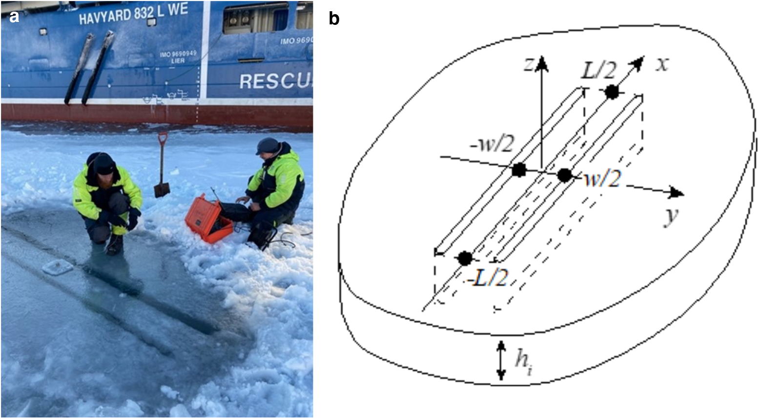
Figure 2. (a) Fixed-ends beam in landfast ice of Tempelfjorden. (b) Schematic of the test with vibrating floating fixed-ends beam.
In contrast to free–free beam or fixed–fixed beam the eigenfrequency of the floating fixed-ends beam is not described by a simple analytical formula. Moreover, the eigenfrequency is complex because elastic energy of the oscillations radiates into the infinity. In addition, the added mass effect should be considered for the modeling of dynamic motions of the floating beam. In the present investigation the elastic modulus was adjusted to the measured frequency by modeling with finite-element software Comsol Multiphysics. Numerical simulations are described in the Supplementary material.
The floating fixed-ends beam was made near the edge of the landfast ice in the Temple Fjord (Fig. 2a) on 9th of March 2022 ~10 km from the geophones (Fig. 1). Preliminary, the ice surface was cleaned from a thin layer of snow. The ice thickness was H = 30 cm. The beam length was L b = 3 m, and the beam width was b = 27 cm. The widths of through cuts in ice was of ~10 cm. We prepared round ends of the cuts using Kovacs drill with 10 cm diameter. The accelerometer was placed in the center of the beam and the beam motion was initiated by several hits by a stick near the beam center.
The ice temperature was measured using a temperature string (Geoprecision) with distance between neighbor thermistors of 5 cm (Fig. 3). The temperature string was placed in natural ice with thin snow layer at the surface. The surface temperature of ice was higher because snow was removed, and ice surface was slightly flooded. We think that ice temperature in the beam was varying between $-2.5^\circ$ C and freezing point of sea water $-1.9^\circ$
 C. Sea ice in the Temple Fjord had columnar structure with diameter of a column of ~1 cm and larger (Fig. 4a). The horizontal thin section in Figure 4b indicated S2 type of ice. The ice salinity was 5 ppt. Speed of p-waves was measured of ~3 km s−1.

Figure 3. Temperature profiles recorded for 5 min for a total duration of 20 min through the sea ice covered by thin snow layer.

Figure 4. Photographs of (a) vertical and (b) horizontal thin sections of sea ice in polarized light. Thin sections were made from a specimen of sea ice from the Tempelfjorden, March 2022. Yellow strips scale 5 cm length.
Record of the beam accelerations is shown in Figure 5. Sampling frequency of the accelerometer was 20 kHz. Accelerations caused by five hits of the beam are well visible in Figure 5a. Figure 5b shows the recorded accelerations up to 0.5 s after the hits were initiated (lines 2–5 are shifted upward for visual purposes), indicating oscillations are the same for each event. Figure 6a shows the spectra of the accelerations recorded during events 1–5, and Figure 6b shows the mean spectrum. One can see that all spectra peaks are located at ~17 Hz. Numerical simulations indicated that eigenfrequency of the fixed-ends beam is 17 Hz when the elastic modulus is of ~1.1 GPa (Supplementary material).

Figure 5. (a) Record of vertical accelerations of the fixed-ends beam versus time during the five events (1–5) initiated by hits of the beam. (b) Zoomed-in records of the acceleration versus time during the five events.

Figure 6. (a) Spectra of acceleration recorded during events 1–5. (b) The mean spectrum of the acceleration.
Figure 7a shows the beam accelerations recorded during 2 s before the first hit shown in Figure 5a. Vibrations of the beam are well visible and spectral analysis shows that the frequency of vibrations was 15.5 Hz in both events I and II (Fig. 4a) without hits. Figure S3b indicates the elastic modulus of 0.9 GPa when the eigenfrequency equals 15.5 Hz. The influence of ice viscosity on the eigenfrequency is expected to be insignificant since the relaxation time of sea ice taken from landfast ice of Spitsbergen fjords was estimated of several tens of seconds and greater (Voermans and others, Reference Voermans2021; Marchenko and others, Reference Marchenko, Karulin, Chistyakov, Karulina and Sakharov2023), which is much larger the period of eigen oscillations of the beam. We may thus conclude that the elastic modulus measured in the test with floating vibrating beam was of about E ≈ 1 GPa.

Figure 7. (a) Accelerations of the beam center versus time during event I. (b) Spectra of the beam accelerations recorded during events I and II.
Data analysis
Source triangulation was used to determine where the vibrations originate from and at what speed the vibrations were propagating. The arrival times of vibration events at the location of the geophones may be determined by:

where t refers to time and (x, y) the coordinates in a relative frame of reference and c is the propagation speed of the waves. Subscripts refer to the geophone (1–3) or the source (0), i.e. t 1 is the instant at which a vibration event arrives at the location of geophone 1 at (x 1, y 1). Equation (1) contains four unknowns (namely, t 0, x 0, y 0 and c) and thus would normally require four geophones to identify where the vibrations are coming from. However, if information is known about the speed at which these vibrations propagate, one more equation is available and the source of the vibration event can be determined with three geophones. In the case of compressive and shear waves, the wave speed is given, respectively, by Stein and others (Reference Stein, Euerle and Parinella1998):

where θ is the Poisson ratio, here taken as 0.3 (e.g. Timco and Weeks, Reference Timco and Weeks2010). For flexural waves in sea ice we assume the ice to be a thin elastic plate such that the dispersion relation of flexural waves in ice can be modeled as (Fox and Squire, Reference Fox and Squire1991; Collins and others, Reference Collins, Rogers and Lund2017):

with L = E*H 3/(12[1 − θ 2]), M = Hρ i/ρ w, where ω = 2π/T is the angular frequency with wave period T, the wave number k and water depth d. From Eqn (3) the propagation speed of wave energy of flexural waves (the group velocity c g) can be determined as c g = ∂ω/∂k. We note that Eqn (3) introduces two additional unknowns, the ice thickness H and effective elastic modulus E*. However, as flexural waves are dispersive, observations of t 1, t 2 and t 3 across a wide range of wave frequencies may provide enough information to determine x 0, y 0, H and E* (e.g. Moreau and others, Reference Moreau, Weiss and Marsan2020b).
We use here two different approaches in estimating the elastic modulus of the ice and the source of vibration events. We focus for this on flexural waves. The first approach considers the difference in arrival times of vibrations with frequency f between pairs of geophones to estimate the group velocity as $c_{{\rm g}, ij}( f) = \left( \sqrt {( x_i-x_0) ^2 + ( y_i-y_0) ^2}-\sqrt {( x_j-x_0) ^2 + ( y_j-y_0) ^2}\right) /$ $( t_i-t_j)$
 , where i and j refer to the geophone numbers. For this, arbitrary (x 0, y 0) are taken to estimate c g(f) for each pair, where solutions for c g(f) and (x 0, y 0) are found when c g,12 = c g,13 = c g,23. For different f, this provides observations of c g across a range of f to which the dispersion relationship Eqn (3) can be fitted. For the second approach, Eqns (1) and (3) are solved iteratively to obtain the lowest RMSE in t 1, t 2 and t 3 with variable (x 0, y 0, t 0), H and E*. We note that alternative approaches exist to the minimum RMSE approach, such as Bayesian inference (Moreau and others, Reference Moreau, Seydoux, Weiss and Campillo2023). The first approach may be seen as local as the phase speed of the vibrations are estimated locally at the site of the geophones, while the second approach may be viewed as non-local as the sea-ice properties between the vibration source and the geophones will influence the results.
Results
In this study, we focus on three major events that were recorded on the 18th, 21st and 22nd of February by all three geophones. We refer to these events as I–III, respectively. In Figures 8a, b the time series of the y- and z-components of geophone 3 during event III are shown. We note that events I and II have similar characteristics as event III, except that the magnitude of the vibrations recorded during event III were the largest. At around t = 170 s, high-frequency vibrations are observed, followed by low-frequency waves over the next few hundred seconds. The high-frequency vibrations are strongest in the horizontal direction and relatively weak in the vertical component, suggesting this may be a compressive wave. The low-frequency waves induces surface velocities similar in magnitude in both horizontal and vertical directions. While magnitude of the voltage amplitudes from t = 400 to 550 s as observed in Figure 8b is increasing, we reiterate that this is not directly translatable to an increased amplitude of the surface elevation of the ice as the geophones response to low frequencies is not linear. In Figure 8c the corresponding time series of sound pressure recorded by the hydrophone is shown. We note that we have shifted the time series of the hydrophone recordings by 65 s to match the records of the geophone loggers. This shift is caused by clock drift as the hydrophone logger, unlike the geophone loggers, is not synchronized by GPS. Based on the audio records, we suspect the event to originate from the glacier and caused by calving (a snapshot of the audio record during this initial event can be found at http://doi.org/10.5281/zenodo.7750699).

Figure 8. Time series of (a) horizontal and (b) vertical vibrations recorded by geophone 3 during event III. A high-frequency event around t = 200 s is closely followed by low-frequency waves between t = 300 and 600 s. Note that the vertical axes are scaled differently. Hydrophone recording during is shown in (c) shifted by 65 s, a shift originating from clock drift of the hydrophone logger, to match the time of the initial vibrations recorded by the geophone loggers.
In Figure 9 the continuous wavelet transform is shown of the time series presented in Figure 8a. The initial vibrations around t = 200 s are within a frequency range of 0.4–18 Hz and do not appear to be dispersive. To obtain information on the times at which these high-frequency vibrations arrived at the geophones, we cross-correlate between the horizontal components of geophone pairs to estimate the transit time of the initial high-frequency vibrations between these pairs, i.e. this will provide estimates of t 1 − t 2, t 1 − t 3 and t 2 − t 3. Following the first approach (see ‘Data analysis’ section), we estimate the propagation speed of these initial vibrations to be 2178, 2184 and 2321 m s−1 for events I–III, respectively, and are coming from the direction of the glacier. We suspect that these vibrations are compressive waves and thus do not satisfy the frequency dispersion relation of Eqn (3).

Figure 9. Continuous wavelet transform of the time series shown in Figure 8a. Color is indicative of the energy, with blue indicating high energy and yellow low energy.
As the low-frequency waves that follow the initial high-frequency vibrations appear to be dispersive (see Fig. 9), and the waves are unlikely to have been generated in the open water, we can obtain the f–t relationship from the wavelet spectrum. For this, we use the wavelet synchrosqueezed transform using Matlab's wsst-function and bump wavelet to identify the times of maximum energy at each frequency (Fig. 10). We note that minima in c g (or maxima in t) can be observed around ~0.14 Hz. From the transit times between each geophone pair and for each wave frequency we can then estimate c g as a function of f. In Figure 11a estimates of c g are compared against the wave dispersion model in sea ice (Eqn (3)) for various values of the ice thickness H and effective elastic modulus E*. For waves with $f\lesssim 0.1$ Hz the propagation speed of waves is largely unaffected by the ice. Notable deviations start to occur for $f\gtrsim 0.11$
 where thicker ice and a larger effective elastic modulus lead to increases in c g. Knowing that the ice thickness near the geophones was measured at ~0.5 m, our initial estimate of E* is 1.4 GPa. This is, however, strongly based on the observations during event I and the frequency range 0.16–0.2 Hz. From the transit times between geophone pairs, i.e. t 1 − t 2, t 1 − t 3 and t 2 − t 3, we can also identify the direction of the source of the waves relative to the geophones (Fig. 11b). Assuming that all waves are supposed to come from the same source for each event, and thus same direction for each event, it suggests that uncertainty in estimates of c g is largest for the higher frequencies.

Figure 10. Wavelet synchrosqueezed transform of the y-component of geophone 3 during events (a) I, (b) II and (c) III, respectively. Color is indicative of the energy, with blue indicating high energy and yellow low energy.

Figure 11. (a) Estimates of group velocity as determined by the transit time between the three geophones for the three wave events. In color are given various estimates of the group velocity based on different effective elastic modulus E* and sea-ice thickness H. (b) Estimates of the direction of the wave source relative to the geophones, where north is taken as 0$^\circ$ .
.
In Figure 12 the dispersion relationship is fitted directly to the observed f−t curves following the second approach (see ‘Data analysis’ section) to obtain best estimates of H and E*. The observations match the dispersion relationship of waves in ice well, although the minima in c g(f) (or maxima in t(f)) tend to be overpredicted (underpredicted). This may, however, also be an artifact of the wavelet synchrosqueezed transform.

Figure 12. Best fits of the dispersion relationship in sea ice (solid line) against observed arrival times at the three geophones for the three events (markers). Note, multiple solutions exist for H–E* that can replicate the best fit, see Figure 13.
As impacts of E* and H on c g are similar for frequencies smaller than about $f\lesssim 1$ Hz, multiple combinations of E* and H can approximate the observations well (Fig. 13). Noting that the ice thickness around the geophones was measured at H ≈ 0.5 m thick, and ice thickness near the glacier may be estimated at about H ≈ 0.75 m based on extrapolation of the ice thickness measurements (a value similar to those measured near the glacier in 2011, e.g. Marchenko and others, Reference Marchenko2011), the average ice thickness through which the vibrations traveled to reach the geophones is ~0.63 m. This would result in best estimates of the elastic modulus as 0.67, 0.64 and 0.42 GPa for events I–III, respectively. This is lower than the measured value of the purely elastic modulus E ≈ 1 GPa at the ice edge from the beam experiments (see ‘Elastic modulus’ section).

Figure 13. Best fit solutions to the wave arrival times as measured by the three geophones for the effective elastic modulus E* and sea-ice thickness H.
The source of the vibrations can be approximated by finding the lowest RMSE fit of the dispersion relation against the f–t curve. Specifically, we find a global minimum for (x 0, y 0) for all three dispersive wave events. Contours of the RMSE for event III are shown in Figure 14 with a best estimate location of the vibration source located near the glacier wall, confirming that the events are originating from the glacier. In Figure 15 the best-estimate source locations of all three events are shown, including the direction of the source of the high-frequency vibrations. We note that the direction of the high-frequency vibration is based on a single data point and is thus expected to be less accurate than the estimate based on the low-frequency waves. They are, nevertheless, consistently directed toward the glacier.

Figure 14. Estimates of the source of the dispersive waves during event III (plus sign) and associated contours of the RMSE of the best fits. Location of the geophones are identified by cross-markers. Sentinel-1 data image taken on 24-02-2022 is given in color.

Figure 15. Estimates of the source of the dispersive waves during events I–III (plus markers) and direction of the high-frequency events (solid lines). Location of the geophones are identified by cross-markers. Sentinel-1 data image taken on 24-02-2022 is given in color.
Discussion
In this study, we estimated the effective elastic modulus from wave observations. We find that the effective elastic modulus derived from fitting the observed wave arrival times to the modeled arrival times retrieves estimates of 0.4–0.7 GPa, whereas estimates based on observations of the group velocity leads to a value of ~1.4 GPa. We believe the former is more accurate given that it uses considerably more data to perform the fitting. Particularly, we see scatter in the direction estimates of the vibration sources relative to the instruments for the higher frequency range (i.e. Fig. 11b), a range fundamental in the fit against the dispersion relationship in ice. However, part of this difference could, possibly, be attributed to the variability of sea-ice conditions, in particular the sea-ice temperature. The sea-ice temperature near the ice edge was measured between −2.5 and −1.5$^\circ$ C (see Fig. 3), and expected to be much lower near the glacier between −15 and −10$^\circ$
 C. Considering either of these estimates, our results suggest that the usage of a default value of E* = 5.5 GPa in wave–ice interaction models may lead to significant errors and/or uncertainties in model simulations as those measured in this study are significantly lower. Further field experiments need to be performed, however, to provide more information on the variability of E* in the field and to provide further recommendations on how to parameterize E*.
While our observations were able to provide estimates of H–E* combinations, details on the ice thickness were required before E* could be estimated explicitly. This is largely because the impacts of E* and H on the shape of the dispersion relationship are indistinguishable for the frequency range of 0.08–0.28 Hz. To illustrate, in Figure 16 we compare Δc g = c g − c g,ref for different points on the H–E* curve for event III (see Fig. 13), with E* = 0.7 GPa and H = 0.54 m taken as the reference group velocity c g,ref. Up to f ≈ 1 Hz the different combinations of H–E* have very limited impact on the shape of c g(f), meaning that the absolute differences in c g for different H–E* combinations are well within the measurement uncertainty of c g. However, if observations are available for f > 1 Hz, the range of H–E* solutions may be reduced significantly as differences in the group velocities between different solutions may exceed 1 m s−1, while for observations of f > 10 Hz we expect that explicit estimates of E* and H become feasible. Although the dispersive waves presented in this study (i.e. Fig. 8) do not contain significant or identifiable energy at f > 0.3 Hz, we note that measurements of dispersive waves at a higher frequency range are frequently encountered in our dataset. For instance, in Figure 17 an example of vibrations caused by a sequence of suspected (thermal) cracks is shown with identifiable phase–time information extending beyond 10 Hz. Usage of such higher frequency vibration events to estimate sea-ice properties was done successfully by others (e.g. Moreau and others, Reference Moreau, Weiss and Marsan2020b; Serripierri and others, Reference Serripierri, Moreau, Boue, Weiss and Roux2022). Unfortunately, no further information of H–E* could be obtained from these data here as these cracking signals were only identifiable in the z-components of the geophones while only two geophones had this component working. Nevertheless, from the continuous wavelet transform we can see that the events arrived first at geophone 2 and we can infer from the data that, taking E* = 0.6 GPa and H = 0.52 m, the source of these cracking events was ~110 m from geophone 2 and 260 m from geophone 3 (see dashed lines in Fig. 17).

Figure 16. Variability of the group velocity Δc g = c g − c g, ref for combination solutions of H–E* with wave frequency. Here, E* = 0.7 GPa and H = 0.54 m are taken for the reference velocity c g, ref. Impact of E* and H to the shape of the dispersion relationship becomes significant for frequencies above 1 Hz.

Figure 17. Example wavelet spectrum of the z-component of the geophone loggers during suspected cracking events. Black dashed line indicates best fit. Color is indicative of the energy, with blue indicating high energy and yellow low energy.
Observations of the elastic modulus from wave observations thus far referred to the effective elastic modulus. However, from the propagation speed of compressive and shear waves in the ice, one may estimate the purely elastic modulus as well (i.e. Eqn (2)). From the direction of the x–y velocity vectors of the geophone signals we may approximate the direction of the initial high-frequency vibration events (Fig. 18). We note that the directions as observed by geophones 2 and 3 are well aligned with the direction from the geophones to the glacier for all three events which supports the hypothesis that the recorded high-frequency vibrations may be compressive waves. However, the direction of the vectors for geophone 1 during these events is consistently shifted by $50$ –$60^\circ$
 for unknown reasons, but we suspect that this is because an error in its alignment during deployment. If we were to assume that these are indeed compressive waves, from Eqn (2) the purely elastic modulus E is then estimated at 3.98, 4.00 and 4.52 GPa for events I–III, respectively. Evaluation of an additional 59 minor high-frequency events in the records shows consistent propagation speeds, with a mean of 2009 m s−1 and standard deviation of 180 m s−1. This is much larger than the in situ estimates of 1 GPa from the beam experiments and we can only speculate on the reason of this difference. Our best guess is that the location and times at which these measurements were taken are too far apart for consistent interpretation. We note that the purely elastic modulus is always larger than the effective elastic modulus, except for very high loading rates where E* will approach the value of E. We find here that E is ~2 and 5–6 times E* for the in situ beam experiments and suspected compressive waves, respectively, and under the conditions experienced during the field experiment. For comparison, Karulina and others (Reference Karulina2019) observed a difference by a factor of 4–5 between measurements of the elastic modulus obtained through cantilever experiments and direct acoustic observations.

Figure 18. Probability density of the vector direction of initial high-frequency vibrations during event I (solid line), event II (dashed line) and event 3 (dash-dot line). North and east correspond to $0^\circ$ and $90^\circ$
 , respectively.
Based on the geophone and hydrophone records, we suspect events I–III to originate from calving events at the glacier wall. The number of reported ice failure events in Spitsbergen glaciers is estimated to be in the range of 50–100 in February based on observations in 2010–12 (Fedorov and others, Reference Fedorov2016), with most events not related to glacier wall calving and occur in the accumulation zone of glaciers. This seems to be consistent with our observations where only three significant events were recorded over a period of ~2 weeks. From this, we may also conclude that ice failure events at a distance from glacier front do not bring energy to the sea ice near the wall.
Although the observations of the low-frequency wave events fit well to the dispersion relationship of flexural waves in sea ice, there are limitations to the methodology used here. Most importantly, we assume here that the wave dispersion model of Fox and Squire (Reference Fox and Squire1991), i.e. Eqn (3), is valid. Second, we assume that the elastic modulus is constant over the ice thickness whilst this is, in general, not the case (e.g. Feltham and others, Reference Feltham, Untersteiner, Wettlaufer and Worster2006). Third, our observations are most likely tsunami events caused by glacier calving, in analogy to landslide-induced tsunamis. The generation of such long waves at such proximity of the instruments are restricted to very limited sites across the polar regions. When waves are generated in open water and cross various types of sea ice, the cumulative impact of the inhomogeneous ice on the group velocity of low-frequency waves makes it problematic to estimate the effective elastic modulus based on the arrival times of waves (i.e. second approach, see ‘Data analysis’ section). In such a case, E* can only be measured by estimating c g from the transit times between the instruments (i.e. first approach, see ‘Data analysis’ section) or using accelerometers as done by, for example Voermans and others (Reference Voermans2021) and Sutherland and Rabault (Reference Sutherland and Rabault2016). Promising approaches that are applicable to sea ice in the MIZ are the derivation of the elastic modulus from dispersive high-frequency vibrations (e.g. Fig. 16) as demonstrated by Moreau and others (Reference Moreau2020a, Reference Moreau, Weiss and Marsan2020b), Serripierri and others (Reference Serripierri, Moreau, Boue, Weiss and Roux2022) and Moreau and others (Reference Moreau, Seydoux, Weiss and Campillo2023). On-board processing and remote data transmission will provide opportunities to increase the currently limited dataset of sea-ice property observations and accelerate the development of parameterizations based on system variables for operational wave forecasting models.
Conclusions
We used observations of low-frequency dispersive waves to estimate the elastic modulus of landfast sea ice. By determining the arrival time of wave events at the geophones and their phase speed, we obtain estimates of the effective elastic modulus of 0.4–0.7 GPa. Estimates of the effective elastic modulus are lower than the purely elastic modulus measured in situ by beam experiments of 1 GPa. Our observation-based estimates of the elastic modulus are significantly lower than the default value of 5.5 GPa currently in use in contemporary wave models. While our observations are by no means representative for all sea ice, our results imply that considerable further efforts are required to increase the database of sea-ice property observations, including observations in the MIZ.
Supplementary material
The supplementary material for this article can be found at https://doi.org/10.1017/jog.2023.63
Acknowledgements
Alexander V. Babanin acknowledges support from the US Office of Naval Research grant N62909-20-1-2080. Joey J. Voermans and Alexander V. Babanin were supported by the Australian Antarctic Program under project 4593. Joey J. Voermans, Jean Rabault, Aleksey Marchenko, Takuji Waseda and Alexander V. Babanin acknowledge the support of the Research Council of Norway and Svalbard Science Forum under project 311266. The authors acknowledge that this work contains modified Copernicus Sentinel data 2022 processed by Sentinel Hub. The acoustic recording of the hydrophone during event III can be found at http://doi.org/10.5281/zenodo.7750699. Firmware and hardware design is made open-source and can be found at http://github.com/jvoermans/Geophone_Logger. All data are made available in an online repository, visit the github repository for further directions on accessing the data or http://doi.org/10.21343/5vhg-a209. The authors thank Ludovic Moreau and an anonymous reviewer whose insightful comments have helped improve this manuscript.
Author contributions
Conceptualization: J.J.V., J.R., A.M., T.N., T.W., A.V.B.; methodology: J.J.V., J.R., A.M.; analysis: J.J.V., J.R., A.M.; writing – original draft: J.J.V.; writing – review and editing: J.J.V., J.R., A.M., T.N., T.W., A.V.B.; supervision: A.M., A.V.B.


 Open access