


Introduction
The accurate representation of subglacial bed topography is important for parameterizing numerous ice-sheet models and analyses. Bed topography is used for calculating ice thickness and determining sea level rise contributions from ice sheets and glaciers (Fretwell and others, Reference Fretwell, Pritchard, Vaughan, Bamber and Barrand2013) and has been shown to play a significant role in determining ice-sheet stability (e.g., Gudmundsson and others, Reference Gudmundsson, Krug, Durand, Favier and Gagliardini2012; Parizek and others, Reference Parizek, Christianson, Anandakrishnan, Alley and Walker2013; Docquier and others, Reference Docquier, Pollard and Pattyn2014; Koellner and others, Reference Koellner, Parizek, Alley, Muto and Holschuh2019), but it remains a major source of uncertainty in ice-sheet projections (e.g., Seroussi and others, Reference Seroussi, Nakayama, Larour, Menemenlis and Morlighem2017). Ice thickness and bed elevation also drive the flow of subglacial meltwater (Shreve, Reference Shreve1972); this subglacial water flow influences ice-sheet movement through the reduction of friction at the bed and contributes to the fast flow of ice streams (e.g., Weertman and Birchfield, Reference Weertman and Birchfield1982; Kamb, Reference Kamb1987; Stearns and others, Reference Stearns, Smith and Hamilton2008).
Bed topography is predominantly measured with airborne radar sounding. Flight profiles are typically spaced several or tens of kilometers apart, thus requiring interpolation (e.g., Fretwell and others, Reference Fretwell, Pritchard, Vaughan, Bamber and Barrand2013). These digital elevation models (DEMs) are commonly constructed with spline or kriging interpolation (Lythe and Vaughan, Reference Lythe and Vaughan2001; Fretwell and others, Reference Fretwell, Pritchard, Vaughan, Bamber and Barrand2013). Kriging is a geostatistical technique that estimates a value by computing the weighted average of nearby points (Cressie, Reference Cressie1990). Because of this averaging, kriging is unable to preserve the variance of the measurements, causing the interpolated topography to be smoother than the observations.
Although kriging-interpolated DEMs provide a useful basis for ice-sheet investigations, Seroussi and others (Reference Seroussi, Morlighem, Rignot, Larour and Aubry2011) found that when kriged bed topography is used with velocity measurements of the ice surface, the modeled flow behavior produces physical inconsistencies. In order to match the surface observations, the ice would have to be losing or gaining mass at unrealistically high rates (Seroussi and others, Reference Seroussi, Morlighem, Rignot, Larour and Aubry2011). Furthermore, the mass flux divergence can exhibit high-frequency variability, which is incompatible with ice flow behavior (Seroussi and others, Reference Seroussi, Morlighem, Rignot, Larour and Aubry2011). To address this discrepancy and ensure flow continuity, a mass conservation interpolation technique can be applied, where bed topography is constrained by bed measurements and ice surface velocity (Morlighem and others, Reference Morlighem, Rignot, Seroussi, Larour, Ben Dhia and Aubry2011; Bamber and others, Reference Bamber, Griggs, Hurkmans, Dowdeswell and Gogineni2013; Morlighem and others, Reference Morlighem, Williams, Rignot, An and Arndt2017). This method enhances interpolations by capturing a greater level of morphological detail that can be done by kriging. With the mass conservation method, topography is selected so that it minimizes the misfit between an ice flow model and observations. This optimization produces a best fit DEM that is not required to reproduce the spatial statistics or heterogeneity of topographic measurements, which can result in smoothing. Furthermore, the mass conservation optimization includes regularization parameters that smooth ice thickness to minimize errors (Morlighem and others, Reference Morlighem, Rignot, Seroussi, Larour, Ben Dhia and Aubry2011), which can exacerbate this smoothing.
The smoothing from kriging or mass conservation interpolation, although typically unavoidable, can bias models of subglacial water flow. Subglacial water routing models are often used to add context to observations and make scientific interpretations (e.g., Siegert and others, Reference Siegert, Le Brocq and Payne2007; Schroeder and others, Reference Schroeder, Blankenship, Young and Quartini2014; Smith and others, Reference Smith, Gourmelen, Huth and Joughin2017). However, these drainage models are limited because they depend on simplified and uncertain bed topography and carry the risk of overinterpretation. Wright and others (Reference Wright, Siegert, Le Brocq and Gore2008) found that ice surface elevation changes of as little as 5 m could dramatically alter meltwater flowpaths and subglacial lake drainage pathways. Furthermore, Chu and others (Reference Chu, Creyts and Bell2016) found that subglacial topographic conditions affect the sensitivity of flowpaths to water pressure changes, thereby determining which flowpaths may be susceptible to rerouting across catchment boundaries. Despite this critical role of topography in controlling subglacial drainage pathways, no method exists for quantifying uncertainty in subglacial water pathways with respect to topographic uncertainty.
The impact of topographic uncertainty on hydrologic uncertainty can be investigated by creating an ensemble of topographic realizations that capture the range of possible bed geometries and have realistic roughness. Each of these topographic realizations can then be used to generate a water routing model, which produces an ensemble of possible subglacial water pathways that can be used for uncertainty quantification. These topographic realizations can be generated with a geostatistical conditional simulation. Conditional simulations are used to generate multiple realizations of a feature while retaining the spatial statistics of observations; they are constrained to measured observations, hence the name ‘conditional’ (e.g., Deutsch and others, Reference Deutsch and Journel1992). In contrast to kriging and mass conservation techniques, which are deterministic methods that solve for the most probable bed elevation at a given point, conditional simulation is a stochastic approach that produces multiple possible solutions with the objective of reproducing the heterogeneity of measurements. The ability of this method to capture heterogeneity is an important advantage for many subsurface investigations. For example, this method is widely used for modeling groundwater hydrology where the spatial distribution of subsurface conditions exerts an important control on flow (e.g., Feyen and Caers, Reference Feyen and Caers2006).
Stochastic modeling is thus a promising tool for ice-sheet investigations, which has prompted several previous studies on subglacial topographic simulation methods and applications (Goff and others, Reference Goff, Powell, Young and Blankenship2014; Graham and others, Reference Graham, Roberts, Galton-Fenzi, Young, Blankenship and Siegert2017; MacKie and others, Reference MacKie, Schroeder, Caers, Siegfried and Scheidt2020; Zuo and others, Reference Zuo, Yin, Pan, MacKie and Caers2020). MacKie and others (Reference MacKie, Schroeder, Caers, Siegfried and Scheidt2020) generated multiple topographic realizations and used these to investigate uncertainty in the surface area and locations of subglacial lakes. Zuo and others (Reference Zuo, Yin, Pan, MacKie and Caers2020) simulated long-wavelength (>10 km) topography and found that, on average, the water flowpath locations in simulated topography differed significantly from those with kriged topography. However, evaluating the sensitivity of water routing to small-scale roughness requires further investigation.
The majority of these previous techniques for generating stochastic simulations of subglacial topography have entailed ‘draping’ synthetic small-scale random roughness onto a DEM with macro-scale topography (Goff and others, Reference Goff, Powell, Young and Blankenship2014; Graham and others, Reference Graham, Roberts, Galton-Fenzi, Young, Blankenship and Siegert2017; MacKie and others, Reference MacKie, Schroeder, Caers, Siegfried and Scheidt2020). The advantage of this approach is that it enables greater control over the interpolation of large-scale topographic features (Goff and others, Reference Goff, Powell, Young and Blankenship2014). However, because this method of simulation involves the addition of small-scale roughness to a smooth underlying DEM, the uncertainty of macro-scale features is not investigated. This addition of small-scale roughness to a smooth underlying surface also means that the simulated topography will not agree with observations; that is, matching the simulated topography to bed measurements requires a considerably greater effort (Goff and others, Reference Goff, Powell, Young and Blankenship2014). Furthermore, no method exists for incorporating mass conservation interpolation estimates into these simulations, leading to the omission of valuable topographic information from these simulations. Uncertainty analysis in glaciology with respect to topographic variability (including, but not limited to, water routing) requires the ability to rapidly generate large ensembles of topographic realizations with the option of incorporating mass conservation estimates, which necessitates a tractable simulation approach.
Our objective in this study is to demonstrate a simple protocol for generating many topographic realizations using mass conservation as a secondary constraint, and to use these realizations to assess hydrologic uncertainty with respect to topographic uncertainty. We demonstrate the first application of this technique to an ice sheet on Jakobshavn Glacier, Greenland. Our results show the effect of topographic perturbations on subglacial water flowpaths. Our methodology is detailed in the sections that follow.
Methods
Topography data
Our study area is located at Jakobshavn Glacier, also known as Sermeq Kujalleq in Greenlandic, in West Greenland (Fig. 1). This site is chosen for its dense radar data coverage and the availability of topography interpolated with mass conservation. The primary data (i.e., known topography values that will not change during the simulations) are acquired from the Center for Remote Sensing of Ice Sheets (CReSIS) radar bed measurements from 2009 (Gogineni, Reference Gogineni2012; Gogineni and others, Reference Gogineni, Yan, Paden and Leuschen2014). We fit the data to a 150 m resolution grid. Our simulation area is 75.15 x 48.90 km2 with a 150 m grid cell resolution. We note that there are additional radar data in this region that are not included in this model. This is due to substantial (>500 m) crossover errors between the 2009 data and subsequent surveys, possibly a result of englacial water that produces false bed reflections or beam pattern asymmetry of off-nadir echoes. These crossover errors are problematic for statistical analyses of bed roughness because they would create an artificially high variance. Therefore, we restrict ourselves to the 2009 data to minimize system, survey and inter-seasonal differences. While we do not consider radar measurement uncertainty in our analysis, we note that it may be significant and thus requires future investigation. The secondary data are obtained from BedMachine Greenland Version 3 (Morlighem and others, Reference Morlighem, Williams, Rignot, An and Arndt2017), which uses mass conservation to interpolate bed topography in this region.
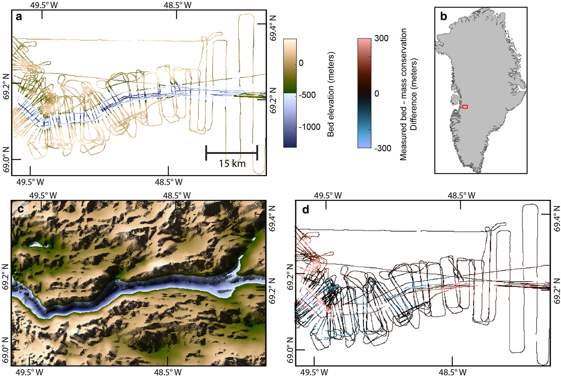
Fig. 1. (a) Primary data from radar measurements (Gogineni, Reference Gogineni2012; Gogineni and others, Reference Gogineni, Yan, Paden and Leuschen2014). (b) Map of Greenland showing study area (Morlighem and others, Reference Morlighem, Williams, Rignot, An and Arndt2017). (c) Secondary data from mass conservation model (Morlighem and others, Reference Morlighem, Williams, Rignot, An and Arndt2017). (d) Radar measurements in (a) subtracted from mass conservation estimates in (c).
Conditional simulation
Sequential Gaussian simulation
The objective of stochastic simulations is to generate realizations of spatial phenomena that reproduce statistical properties observed in the data set. A commonly used descriptor of spatial statistics is the variogram, which measures the covariance between two locations as a function of lag distance. The theoretical definition of a variogram is
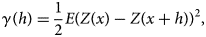
where x is a spatial location, Z(x) is a variable, and h is the lag distance. The empirical variogram $\hat {\gamma } \, \lpar h\rpar$ is calculated from locations x α for N number of points as

Typically, this variance increases with increasing lag distance. To generate realizations that reflect the degree of variance increase observed in the variogram, we perform simulations using a sequential Gaussian simulation (SGSIM) (Deutsch and others, Reference Deutsch and Journel1992; Goovaerts and others, Reference Goovaerts1997). SGSIM produces many realizations of the spatial phenomenon, while reproducing the spatial variation modeled with the variogram. In addition, known values (i.e., radar measurements) are not altered by the simulation. The set of realizations quantifies the spatial uncertainty of topography.
SGSIM begins by performing a normal score transformation on the elevation measurements so that they resemble a standard Gaussian distribution. SGSIM uses the variogram to determine the mean and variance at the pixel of interest, which define a normal probability distribution of elevation values at this location. While kriging interpolation selects the mean from this distribution, SGSIM draws a value from the Gaussian distribution that becomes the simulated elevation at that pixel. This simulated value is then assimilated into the conditioning data and is used to estimate the mean and variance at the next simulation pixel. SGSIM uses a random path to sequentially visit each pixel, compute the probability distribution, and simulate an elevation value; this process is repeated until every pixel has been simulated. Thus, the smoothing effect of kriging is avoided. The standard Gaussian simulation is then back-transformed so that the original elevation distribution is recovered.
The SGSIM method is suitable when a single variable (e.g., radar bed elevation measurements) is available. However, because this study integrated two sources of information, radar and mass conservation, we use a modified method of SGSIM known as sequential Gaussian co-simulation (CO-SGSIM) (Verly, Reference Verly1993; Almeida and Journel, Reference Almeida and Journel1994). CO-SGSIM is modified from SGSIM to model the posterior distribution based on multiple sources of information (Fig. 2). The radar bed measurements are a primary source, while the mass conservation topography is a secondary source. Each source undergoes a normal score transformation and is associated with a spatial process or random function. Z 1(x), also termed the primary variable, describes the target spatial variable, in this case, radar measurements. Z 2(x) represents the secondary variable, the mass conservation topography.
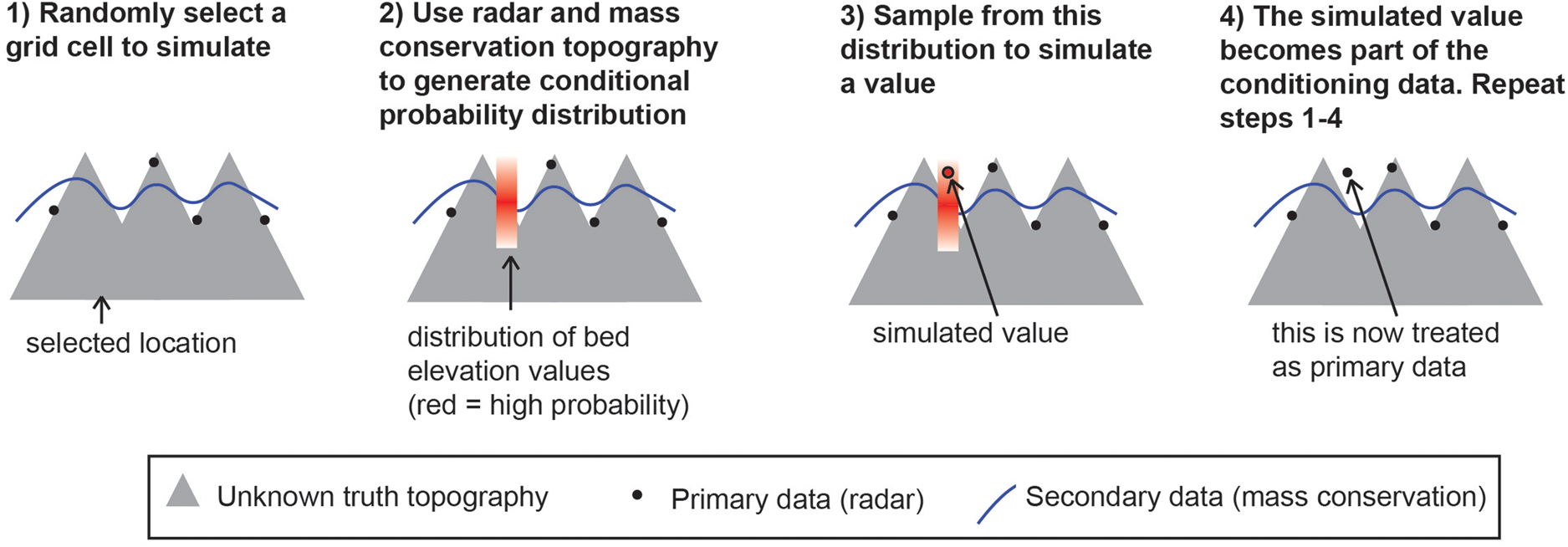
Fig. 2. Schematic of CO-SGSIM. The radar and mass conservation topography (1) are used to generate a local conditional probability distribution (2). Then a value is randomly selected from this distribution (3), which is then assimilated into the conditioning data (4). These steps are repeated until every grid cell has been simulated.
Modeling joint spatial variation
While SGSIM uses kriging as an estimator, CO-SGSIM uses cokriging. Cokriging is a multivariate form of kriging that is used to estimate a sparsely-sampled primary variable (radar) in the presence of a well-sampled secondary variable (mass conservation). In contrast to kriging, which requires the modeling of only one variogram, cokriging is implemented by producing variograms for each variable, as well as a cross-variogram describing their joint spatial variation. Like the variogram, the cross-variogram describes the covariation between observations at two locations, but now between two different variables. The cross-variogram between two variables cannot be defined independently of their respective variograms because the variables are spatially interdependent (Cressie, Reference Cressie1990). Specifically, in order for the simulated topography to retain both the variogram of the radar measurements and its correlation with the mass conservation estimates, we must account for redundancy between the two variables. However, solving the full cokriging system is difficult in practice because it is computationally expensive and can result in negative variances (e.g., Almeida and Journel, Reference Almeida and Journel1994; Journel, Reference Journel1999).
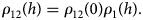
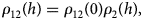
The cross-variogram can be approximated through a Markov-type assumption of conditional independence between variables. Journel (Reference Journel1999) defines two such Markov models, Markov Model 1 (MM1) and Markov Model 2 (MM2). MM1 assumes that a secondary datum Z 2(x) is conditionally independent of Z 1(x + h) (Almeida and Journel, Reference Almeida and Journel1994; Journel, Reference Journel1999). In other words, the mass conservation estimate, given a corresponding radar measurement, is independent of radar measurements at other pixels. MM1 is a very simple and attractive model because only the primary correlogram ρ 1(h) and the correlation coefficient ρ 12 = ρ 12(0) between the primary and secondary data need to be calculated. The correlogram is a standardized form of the variogram; it is used because the variables have been converted to standard Gaussian distributions. Then the cross-correlogram model is calculated simply as
Note that under assumptions of variogram and variance stationarity, the relation between a correlogram and a variogram is as follows:

where Var(Z) is the variance of Z. Therefore, for MM1, we only need to model the variogram for the radar data and calculate the correlation coefficient between the radar observations and mass conservation estimates; the variogram for the secondary data does not need to be modeled. MM1 is frequently used because it is easy to implement. However, MM1 makes the assumption that the primary variable varies more slowly than the secondary variable. Often, due to this assumption, the resulting realizations have an artificially high variance. Furthermore, MM1 screens out the influence of primary data on the secondary data, except at the pixel of interest, which causes the redundancy between the primary and secondary data to be underestimated. This can produce realizations that correlate too strongly with the secondary data (Shmaryan and Journel, Reference Shmaryan and Journel1999).
To avoid these issues, an alternative Markov model, MM2 (Journel, Reference Journel1999) can be applied. MM2 assumes that the primary variable at the pixel of interest is conditionally independent of the secondary data values at other pixels. In other words, it is assumed that a radar bed measurement at a certain pixel, given a corresponding mass conservation estimate, is independent of mass conservation values at other pixels. MM2 assumes that the primary spatial variable is the sum of the secondary spatial variable and some residual term. This residual term explicitly acknowledges that the primary variable is more varying than the secondary variable. In that case, theory states that
and the primary correlogram is defined as

The variogram or correlogram models under MM2 are more difficult to obtain than in MM1 because they require some additional variogram modeling of the residual variogram ρ R(h). Once the variograms for radar, mass conservation and their cross-covariation are defined, the cokriging estimate can be made, and random sampling from the posterior distribution described by these parameters is used to produce Monte Carlo simulations of topography. Each simulated realization will then reproduce all the parameters of the Gaussian process, including their cross-correlation, as observed in the data. The realizations are then automatically back-transformed to recover the original elevation distribution. We tested both Markov models on our case study and investigated the validity of each to determine the best model with which to generate an ensemble of 250 simulations.
Variogram analysis and simulation implementation
We use the Stanford Geostatistical Earth Modeling Software (Remy, Reference Remy2005) to estimate the variograms and conduct the simulations. See Remy (Reference Remy2004) and Remy and others (Reference Remy, Boucher and Wu2009) for detailed documentation on implementation. The MM1 simulation is initialized by (1) transforming the variables to standard Gaussian distributions, (2) calculating ρ 12(0) and (3) modeling the primary variogram. The MM2 simulation requires the additional step of modeling the secondary variogram; the primary variogram is modeled by defining a residual variogram between the primary and secondary varaible (Fig. 3). The following are the modeled variograms:
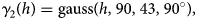
and

where gauss(h, a max, a min, β) refers to a 2D Gaussian model with a major range a max (in grid cells, where each grid cell is 150 m), a minor range a min, and azimuthal direction β of the major range. sph(h, a max, a min, β) refers to a spherical model (Smith, Reference Smith2011). By specifying the major and minor ranges, we account for anisotropy. We found that the correlation coefficient ρ 12(0) is 0.78. Once the variograms are defined, the simulations are implemented using the CO-SGSIM tool in the Stanford Geostatistical Earth Modeling Software.
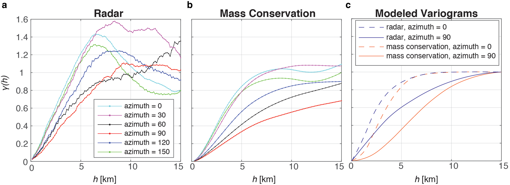
Fig. 3. Normal score variograms for radar (a) and mass conservation topography (b) for various azimuthal directions. (c) Modeled variograms for radar and mass conservation for the MM2 simulation.
Water routing
We investigate the sensitivity of subglacial water flow to topography by generating a water routing model for the initial, unmodified mass conservation DEM and each topographic realization. The water routing model is determined by calculating hydraulic potential, ϕ, using the Shreve equation (Shreve, Reference Shreve1972):
where ρ w is the density of water (1000 kg m−3), ρi is the density of ice (917 kg m−3), g is gravitational acceleration, h is bed elevation and H is ice thickness. We use the Antarctic Mapping Tools (Greene and others, Reference Greene, Gwyther and Blankenship2017) and the FLOWobj function and multiple flow directions (MFD) algorithm from the TopoToolbox package (Schwanghart and Scherler, Reference Schwanghart and Scherler2014) to delineate subglacial water drainage pathways based on subglacial hydropotential gradients and calculate flow accumulation. Our routing model assumes the subglacial water source is spatially uniform basal melt. This model makes the idealized assumption that the water pressure is always equal to the ice overburden pressure, the implications of which are addressed in the Discussion section.
Results
The MM1 realization contains interpolation artifacts; these artifacts are minimized in the MM2 realization (Fig. 4). Specifically, the realization made using MM1 exhibits irregularities where radar measurements were taken and lacks a seamless transition between the radar measurements and the simulated data. Given these results, our ensemble of 250 realizations was generated using MM2.
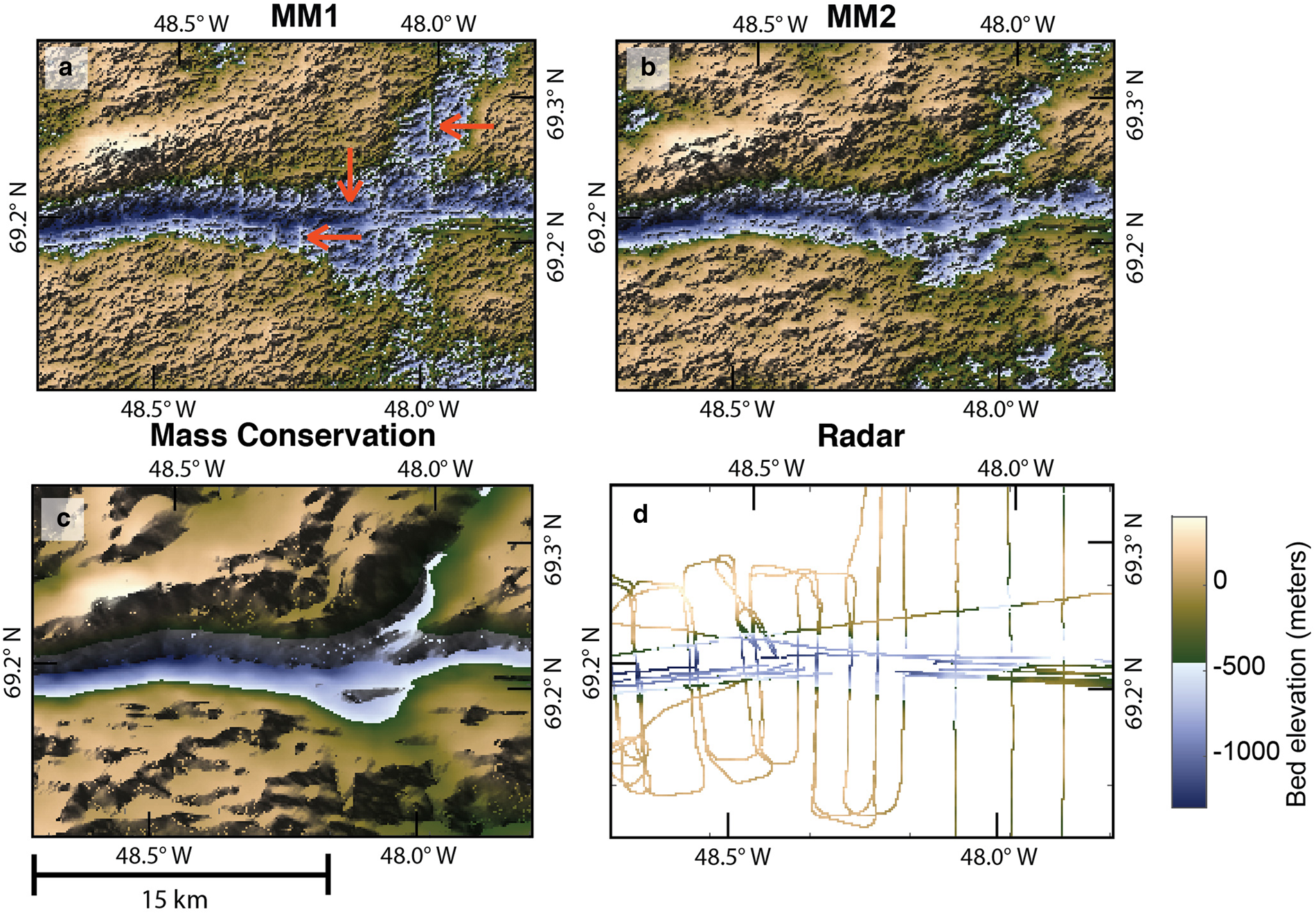
Fig. 4. Zoomed in comparisons of Markov model 1 (a) and MM2 (b). The mass conservation topography (c) and radar measurements (d) are shown for comparison.
The ensemble realizations have large-scale features similar to those of the mass conservation DEM, but they are substantially rougher (Fig. 5). The average of the realizations is similar to that of the mass conservation DEM (Fig. 6a). The standard deviation for bed elevation is zero where there is a radar measurement and is upwards of 300 m in those regions that are more than several kilometers from a data point (Fig. 6b).
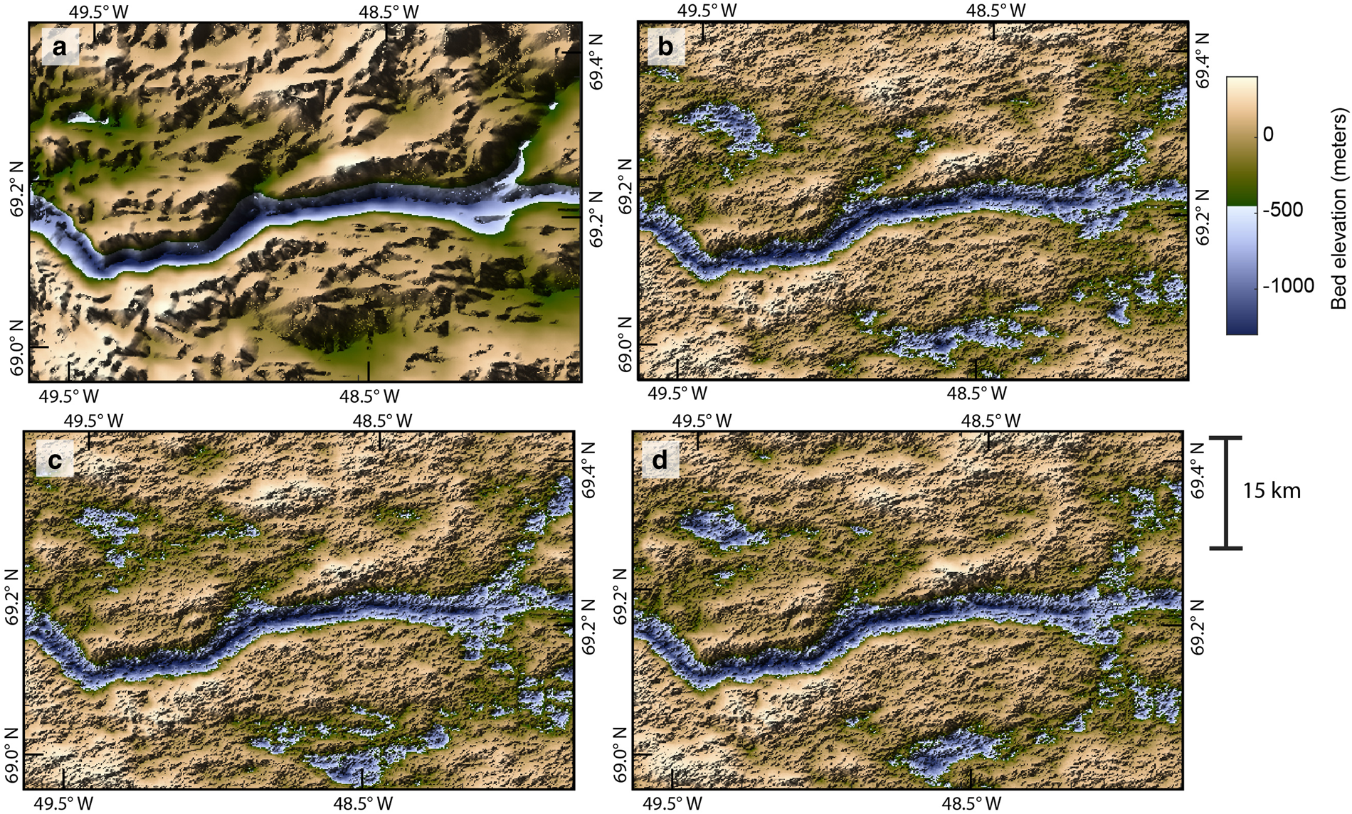
Fig. 5. (a) Mass conservation DEM. (b–d) Sample realizations using MM2.
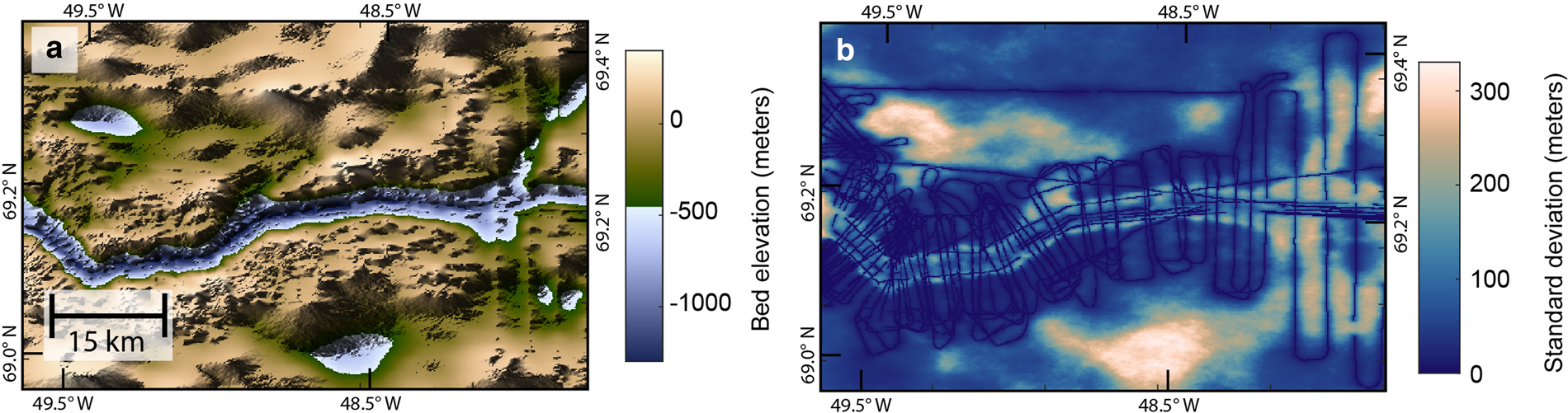
Fig. 6. (a) Mean of simulations. (b) Variance of simulations. A variance of zero indicates the presence of radar measurements.
In each DEM, there is a water flowpath in the main trough in the center of Jakobshavn Glacier (Fig. 7). The numbers and locations of the adjoining tributaries differ in each DEM. The average of the water routing models (Fig. 8) shows that, while the main channel is repeated across realizations, the locations of the smaller branches are more variable. The mean flow accumulation values in Figure 8b appear blurred in the upstream areas and become more defined moving downstream. Figure 8d shows that some of these pathways are more repeatable across some realizations than they are across others. The topography results are available in a data repository: https://doi.org/10.5281/zenodo.3875144.
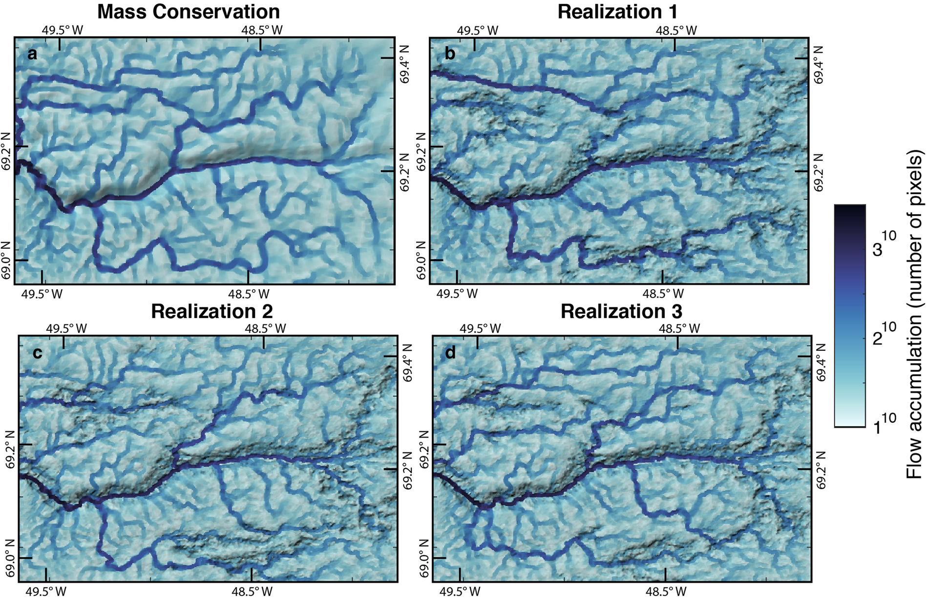
Fig. 7. Subglacial water flowpaths for DEMs in Figure 5 with mass conservation topography (a) and the first three geostatistical realizations (b–d). This shows that the main channel is reproduced in each DEM, whereas smaller tributaries vary across realizations. The water routing is superimposed on hillshade topography and plotted on a power 10 scale for visualization.
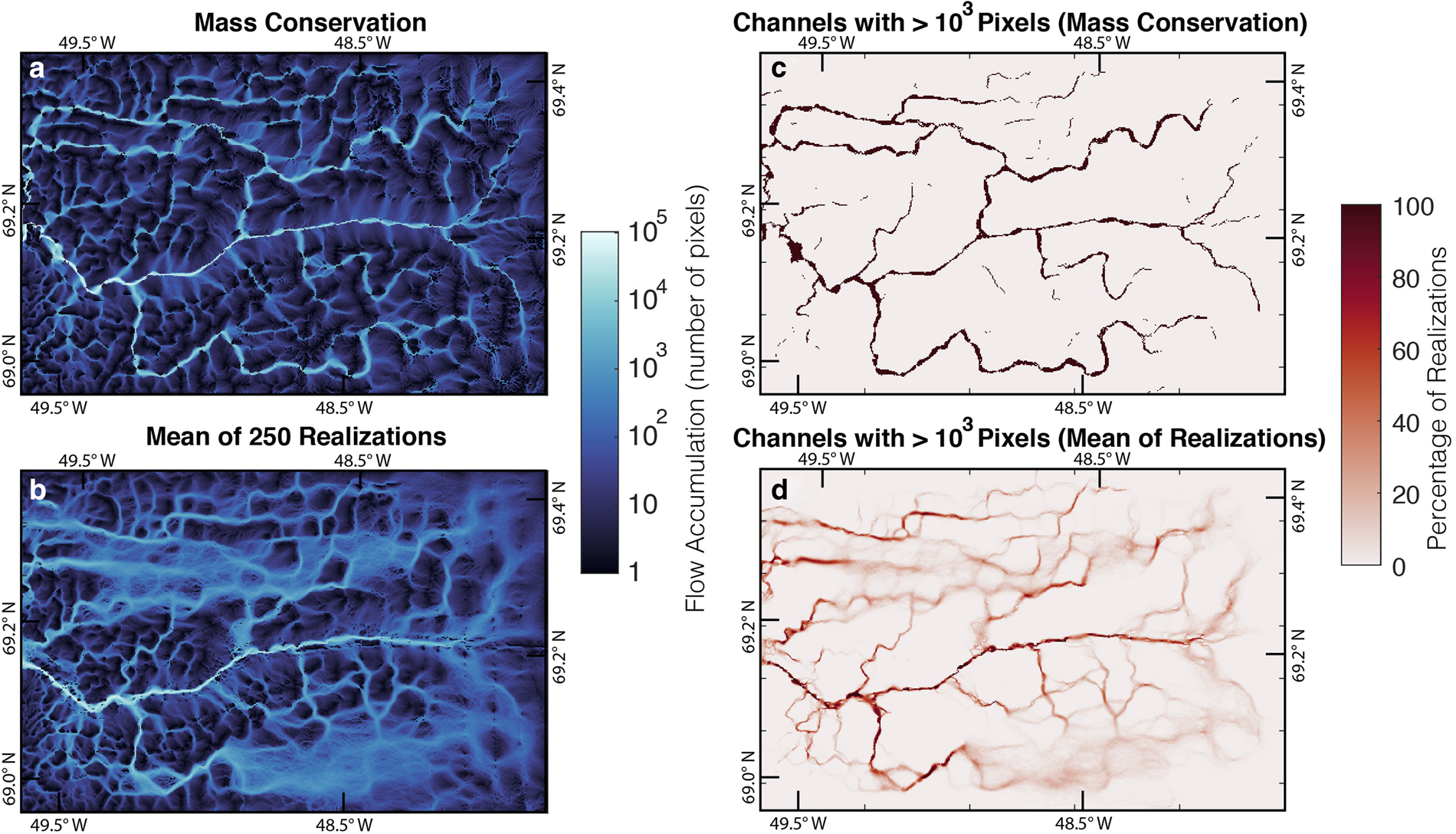
Fig. 8. (a) Flow accumulation for mass conservation DEM. (b) Mean of flow accumulation values across realizations. (c) Mass conservation flow paths with > 1000 contributing pixels. (d) Percentage of realizations with flow accumulation values > 1000 at a given point.
Discussion
Our results demonstrate that stochastic modeling offers an approach to quantifying uncertainty in subglacial hydrologic systems. The sequential Gaussian co-simulation method allows us to combine the roughness of radar bed topography measurements with the large-scale topographic features from mass conservation to conduct stochastic simulations of topography. This method can be easily used to generate multiple realizations, enabling uncertainty quantification in bed elevation and other variables that depend on topography.
Our simulations show the robustness (or lack thereof) of water routing pathways to topographic uncertainty, subject to the assumptions of a subglacial drainage system at ice overburden pressure. Depending on the DEM, significant variations can occur in subglacial drainage pathways. In our study, the flowpath in the main trough persisted across different realizations. Other pathways were also repeatable, but at lower frequencies (Fig. 8d). Therefore, water routing models should be treated with care when used to interpret observations, and only flowpaths along dominant topographic features can be assumed with great confidence to have water flowing through. Figure 8b shows that flowpaths became increasingly uncertain as they moved further away from the main trough, though the flowpaths across different realizations converged going downstream toward the primary channel. This convergence suggests that upstream uncertainty does not propagate downstream when meltwater flows toward a major topographic feature. We note that the trough at Jakobshavn Glacier is unique, and most subglacial settings would have even greater uncertainties in flowpaths. This information could be used when planning radar surveys in order to optimize the reduction in hydrologic uncertainty.
Our hydrological model assumes that the water pressure equals the ice overburden pressure, though there is existing evidence to the contrary. Borehole observations have shown diurnal and seasonal fluctuations in water pressure (Fudge and others, Reference Fudge, Humphrey, Harper and Pfeffer2008; Meierbachtol and others, Reference Meierbachtol, Harper and Humphrey2013). Moreover, theoretical modeling has demonstrated that channelization can occur at high discharge rates (Werder and others, Reference Werder, Hewitt, Schoof and Flowers2013), creating pressure gradients that may override the effect of the added topographic roughness. Our approach does not capture these processes. Rather, we provide a simple demonstration of how stochastic modeling can be used to investigate hydrological uncertainty. Our analysis could be easily adapted to consider more complex subglacial flow regimes.
Stochastic modeling could provide insights into the characteristics of subglacial water systems. At low water pressures, the sensitivity of subglacial water flow to pressure variations is largely dependent on subglacial bed slope (Chu and others, Reference Chu, Creyts and Bell2016), so topographic simulations could be used to determine which areas might be sensitive to rerouting. Ensemble topographic and hydrological simulations could highlight ambiguity in catchment delineations or be used to assess the potential for water piracy across catchment boundaries, which has been hypothesized to be possible in West Greenland under certain conditions (Chu and others, Reference Chu, Creyts and Bell2016). Uncertainty quantification in catchment delineations could also be used to investigate meltwater budgets. Imbalanced meltwater budgets are often attributed to subglacial and englacial water storage (e.g. Rennermalm and others, Reference Rennermalm, Smith, Chu, Box and Forster2013), though it could also be explained by flowpaths draining in different locations. Ensemble simulations of subglacial flowpaths could also add important context to bed measurements. For example, knowing the likelihood that water flows down a certain pathway could affect the placement and interpretation of geophysical observations (e.g., borehole, radar or seismic measurements).
This method of topographic simulation could also enable a wide range of ice-sheet investigations. Multiple realizations of bed topography would allow for uncertainty quantification in ice-sheet volume and sea level rise contribution. Ensemble topographic realizations could also be used in ice-sheet models to quantify uncertainty in projections of ice-sheet retreat with respect to topographic uncertainty. For example, stochastic modeling could be used to investigate uncertainties in topographic ridges and pinning points, which are known to have a buttressing effect on glaciers (e.g., Favier and others, Reference Favier, Gagliardini, Durand and Zwinger2012; Parizek and others, Reference Parizek, Christianson, Anandakrishnan, Alley and Walker2013).
Our variogram models specify major and minor range axes, which allows for anisotropy. It is important to consider anisotropy in simulations of subglacial topography, given that morphological investigations show that topographic features are strongly aligned with ice flow direction (e.g. Spagnolo and others, Reference Spagnolo, Bartholomaus, Clark, Stokes and Atkinson2017). We do not, however, define variograms for multiple orientations or account for locally varying anisotropy, although techniques exist for incorporating locally varying anisotropy into simulations (e.g., Boisvert and Deutsch, Reference Boisvert and Deutsch2011) that could be applied to this method. CO-SGSIM might not be applicable over large areas with highly variable spatial statistics (non-stationarity). Nevertheless, CO-SGSIM is an efficient and effective method for investigating uncertainty in small areas, though further work is needed to generate simulations of more complex environments.
In our experiments, Markov Model 2 performed better than MM1. The artifacts in MM1 (Fig. 4) are likely a result of the known issue that MM1 realizations have a tendency to over-correlate with the secondary variable; this makes the flight lines stand out. The artifacts are still visible in MM2, though to a far lesser degree. The MM2 artifacts may stem from non-stationarity in the topography, which we do not account for. They could also be attributed to closely spaced, cross-cutting flight lines (Fig. 4d) that may contain crossover errors.
Although radar crossover errors can be up to several hundreds of meters, our simulation does not consider observational uncertainty. We omitted conflicting radar surveys in our study area because these crossover errors would bias the variogram toward higher roughness. Future work is needed to accurately model variograms for datasets with crossover errors. Measurement uncertainty is often estimated through crossover error analysis (e.g., Gogineni and others, Reference Gogineni, Yan, Paden and Leuschen2014). However, the magnitudes of crossover errors can vary greatly throughout a region. Specifically, large crossover errors attributed to off-nadir reflections are more likely to occur in areas with rough or complex topography. Therefore, topographic roughness could be used to help generate locally varying estimates of measurement uncertainty. We also do not use existing mass conservation uncertainty estimates, though this can be explicitly quantified (e.g., Morlighem and others, Reference Morlighem, Rignot, Seroussi, Larour, Ben Dhia and Aubry2011; Brinkerhoff and others, Reference Brinkerhoff, Aschwanden and Truffer2016). Future stochastic modeling efforts could directly use radar and mass conservation uncertainties to model the posterior elevation distribution.
Our method is informed by mass conservation, but it does not necessarily obey mass conservation laws or maintain the flow continuity of mass conservation DEMs. Further research is needed to assess the effects of simulated topography on ice flow behavior. This method has the same limitations as the mass conservation technique: it is only effective in regions of high ice velocity, and it relies on assumptions about basal sliding (Morlighem and others, Reference Morlighem, Rignot, Seroussi, Larour, Ben Dhia and Aubry2011). In addition, this technique is also dependent on the availability of mass conservation topography. In regions that lack a mass conservation estimate (e.g., inland Greenland where the ice velocity is low), SGSIM could be used instead of CO-SGSIM.
Conclusions
Subglacial topography and hydrology are important parameters in numerous investigations of ice sheets, but they have potentially large uncertainties that are difficult to quantify. We have demonstrated the application of established geostatistical techniques to subglacial topography in order to simulate ensemble bed realizations. These DEMs and the conditioning data are publicly available at https://doi.org/10.5281/zenodo.3875144. We found that subglacial drainage flowpaths are very sensitive to topographic variations and that water routing models from kriging or mass conservation DEMs should be interpreted with extreme care. The method presented here could be used to contextualize bed measurements or to gain insights into the stability of subglacial flowpaths and the potential for rerouting. Although future work is needed to address observational uncertainty and develop simulation techniques for locations where the spatial statistics are highly variable, this method of stochastic simulation provides a path forward for quantifying hydrologic uncertainty.
Acknowledgements
We thank Thomas Teisberg and Mary McDevitt for thoughtful feedback on the manuscript. We also thank Douglas Brinkerhoff and an anonymous reviewer for the constructive comments that greatly improved the final manuscript. See https://doi.org/10.5281/zenodo.3875144 for data products generated in this study.


 Open access