


1. Introduction
Meltwater under a glacier or ice sheet affects how quickly the ice flows into the ocean. On the Greenland Ice Sheet, which holds 7 meters of global sea level, this subglacial water is sourced from both basal melt (~21 Gt a−1; Karlsson and others, Reference Karlsson2021) and surface melt (~260 Gt a−1; Fettweis and others, Reference Fettweis2020). Given the importance of surface melt to the basal environment, monitoring the transfer of surface water to the bed is essential to predicting ice flow and sea-level rise sourced from glaciers and ice sheets.
Across much of Greenland, surface meltwater flows across the ice-sheet surface into crevasses or moulins that take the water to the bottom of the ice sheet (Smith and others, Reference Smith2015). In certain areas, however, high snowfall rates can bury meltwater and insulate it from the winter cold (Kuipers Munneke and others, Reference Kuipers Munneke, Ligtenberg, van den Broeke, van Angelen and Forster2014). These conditions can give rise to firn aquifers – liquid water reservoirs tens of meters beneath the surface, where meltwater saturates the firn host material (Forster and others, Reference Forster2014). These firn aquifers are invisible from the surface, yet are estimated to cover from 22 000 to 70 000 km2 (Forster and others, Reference Forster2014; Miége and others, Reference Miége2016; Brangers and others, Reference Brangers2020; Miller and others, Reference Miller2020) and hold as much as 140 Gt (140 km3) of liquid water (Koenig and others, Reference Koenig, Miége, Forster and Brucker2013; Chu and others, Reference Chu, Schroeder and Siegfried2018).
Firn aquifers exist in locations on the Greenland Ice Sheet with specific climatic conditions: warm ($> 0^\circ$ C) summer air temperatures that give rise to meltwater that percolates downward into the snow and firn, and high winter snowfall rates (>~0.6 m water equivalent per year), which insulate the meltwater from cold winter air temperatures above and prevent it from refreezing (Kuipers Munneke and others, Reference Kuipers Munneke, Ligtenberg, van den Broeke, van Angelen and Forster2014; Meyer and Hewitt, Reference Meyer and Hewitt2017; Ligtenberg and others, Reference Ligtenberg, Miége, MacFerrin and van den Broeke2018). These conditions are met primarily in Southeast Greenland, Northwest Greenland and small areas in South and Southwest Greenland (Miége and others, Reference Miége2016). Firn aquifers are also found on alpine glaciers (e.g., Fountain, Reference Fountain1989; Ochwat and others, Reference Ochwat, Marshall, Moorman, Criscitiello and Copland2021), Svalbard ice fields (Christianson and others, Reference Christianson, Kohler, Alley, Nuth and Pelt2015), and ice shelves on the Antarctic Peninsula (Montgomery and others, Reference Montgomery2020; van Wessem and others, Reference van Wessem, Steger, Wever and van den Broeke2021).
Firn aquifers contain both liquid water and solid ice in the form of firn, with water comprising 5–20% of the aquifer by volume (Koenig and others, Reference Koenig, Miége, Forster and Brucker2013; Miller and others, Reference Miller2021). The first Greenland firn aquifer was discovered by collecting ice cores (Koenig and others, Reference Koenig, Miége, Forster and Brucker2013; Forster and others, Reference Forster2014). Since then, the location of the water table – the top surface of the firn aquifer – has been mapped over the entire ice sheet using airborne radar (Forster and others, Reference Forster2014; Miége and others, Reference Miége2016). In a pioneering and comprehensive study, Miége and others (Reference Miége2016) used airborne radars flown on NASA's Operation IceBridge (OIB) over 2010–2014 to map the firn-aquifer water table across the ice sheet. They located 22,000 km2 of firn aquifers around the Greenland Ice Sheet and identified the water table across five seasons. They found that the depth to the water table ranges from 5–40 m and averages 22 m. At a given location, the water table tends to be steady from year to year (Miége and others, Reference Miége2016; Chu and others, Reference Chu, Schroeder and Siegfried2018), but variations of a few meters have been observed, including a rise in water table by 1.1 m at a well-studied location near Helheim Glacier following the high melt year 2012, and a lowering by 2.5 m there due to an inferred water drainage event in 2014 (Miége and others, Reference Miége2016). Chu and others (Reference Chu, Schroeder and Siegfried2018) observed variations of 4–15 m at this location, which, like Miége and others (Reference Miége2016), they ascribed to a combination of changes in recharge and downstream drainage.
Firn aquifers occupy a relatively narrow band on the ice sheet, dictated by climatic conditions as described above, that sits roughly between 1500–2000 m elevation (Howat and others, Reference Howat, Negrete and Smith2014, Reference Howat, Negrete and Smith2022; Kuipers Munneke and others, Reference Kuipers Munneke, Ligtenberg, van den Broeke, van Angelen and Forster2014; Miège and others, Reference Miége2016). The upglacier boundary of a firn aquifer tends to be diffuse in space; it is likely set by climatic conditions – summer melt and winter snowfall rates – as well as surface topography (Miége and others, Reference Miége2016). Recent studies suggest that this upglacier boundary is migrating farther inland in response to climate warming (Steger and others, Reference Steger, Reijmer and van den Broeke2017; Chu and others, Reference Chu, Schroeder and Siegfried2018; Miller and others, Reference Miller2020). At the downglacier boundary, on the other hand, the water table often terminates abruptly (Miége and others, Reference Miége2016). In some radar images, crevasses are visible as bright, shallow, vertically oriented reflectors that appear at this downglacier boundary (Miége and others, Reference Miége2016), but they do not appear consistently at all downglacier boundaries. This is likely because the radar is not well suited to resolving vertically oriented features such as crevasses, so detection of crevasses by OIB radar is not reliable. To date, no study has investigated the relationship between crevasses and the downglacier termination of the firn aquifer at a regional scale.
The end of NASA's OIB and its airborne radar profiling in 2020 left the community without an immediate means to monitor Greenland firn aquifers. Thus, multiple research groups developed new methods for remote sensing these firn aquifers by satellite. Miller and others (Reference Miller2021) identified Greenland firn aquifers by analyzing the time evolution of brightness temperature observed by L-band microwave radiometer. This differs from analyzing airborne (Miége and others, Reference Miége2016) or ground-penetrating radar (Christianson and others, Reference Christianson, Kohler, Alley, Nuth and Pelt2015) data, making improvements via improved spatio-temporal coverage, but achieving coarser spatial resolution (~18 km) and encountering new difficulties resolving the firn-aquifer boundary (Miller and others, Reference Miller2020). Similarly, Brangers and others (Reference Brangers2020) analyzed the time evolution of spaceborne Sentinel-1 C-band synthetic aperture radar backscatter data to identify firn aquifers. Their technique covers the entire ice sheet and greatly improves the spatial resolution to 1 km2, but the radar only penetrates a few meters into the ice sheet, meaning that it cannot sense the water table directly. Instead, both Brangers and others (Reference Brangers2020) and Miller and others (Reference Miller2020, Reference Miller2021) infer the presence of a firn aquifer by evidence of near-surface melt (low backscatter and brightness temperature, respectively) that persists beyond the melt season.
These advances in remote sensing of firn aquifers have increased our knowledge of these features across Greenland. Only a small area, however, has been studied in detail through field work and numerical modeling (Forster and others, Reference Forster2014; McNerney, Reference McNerney2016; Miller and others, Reference Miller2017a, Reference Miller2017b; Poinar and others, Reference Poinar2017; Legchenko and others, Reference Legchenko2018; Miller and others, Reference Miller2020, Reference Miller2022). At this site ~40 km upglacier of the terminus of Helheim Glacier in Southeast Greenland, modeling studies show that the firn aquifer drains its water to the glacier bed through wide crevasses that penetrate to the glacier bed (McNerney, Reference McNerney2016; Miller and others, Reference Miller2017a; Poinar and others, Reference Poinar2017). This drainage is unique because it occurs farther upglacier, well above the equilibrium line, than any other known site in Greenland where meltwater regularly reaches the bed (Poinar and others, Reference Poinar2015; Stevens and others, Reference Stevens2015). This unique upglacier water source allows for a steadier, more efficient subglacial hydrologic system year-round (Poinar and others, Reference Poinar, Dow and Andrews2019).
It is not currently known, however, whether crevasses allow drainage of the firn aquifer in locations other than the well-studied Helheim Glacier site. Indeed, firn-aquifer water may meet other fates in other areas, as illustrated in Figure 1. These could include discharge back to the ice-sheet surface in the form of small lakes analogous to groundwater seeps (Figure 1b, Dunmire and others, Reference Dunmire, Banwell, Wever, Lenaerts and Datta2021) or refreezing englacially at the base of the aquifer dozens of meters below the ice-sheet surface (Figure 1c, Meyer and Hewitt, Reference Meyer and Hewitt2017; Miller and others, Reference Miller2020). In these two cases, meltwater in the firn aquifer would stay in the near-surface environment without reaching the bed, and therefore would not have a measurable effect on ice dynamics. Thus, it is important to identify regions where crevasses potentially connect firn-aquifer water to the bed (Fig. 1a) and regions where they do not (Fig. 1b–c). Overall, data that inform where Greenland firn aquifers drain to the glacier bed are needed in order to constrain the evolution of the subglacial hydrologic system that controls ice flow above (Poinar and others, Reference Poinar, Dow and Andrews2019; Sommers and others, Reference Sommers2022).

Figure 1. Schematic illustrations of three possible hypotheses for the fate of water at the downglacier boundary of a firn aquifer. In cross sections (left column; not to scale), firn-aquifer water is represented by the blue area inside the ice sheet (white). Refreezing in the aquifer is illustrated by fading from blue to white. In plan views (right column; to scale), firn-aquifer water is shown as blue polygons overlain on a World Imagery basemap from ESRI in ArcMap (ESRI and others, 2009). Inset (left) shows locations of all panels (red squares). (A) Illustration of our primary hypothesis, that water at the downglacier boundary flows into crevasses (dark blue) and hydrofractures downward. In plan view, these crevasses are colored red. (B) Illustration of the secondary hypothesis, that water at the downglacier boundary returns to the surface or near surface as a shallow subsurface lake or spring. Subsurface lake boundaries from Dunmire and others (Reference Dunmire, Banwell, Wever, Lenaerts and Datta2021) in plan view are light green. (C) Illustration of the tertiary hypothesis, that water in the firn aquifer refreezes into the firn and ice immediately beneath and downglacier.
Crevasses substantially wider than a few meters likely contain liquid water (Meier and others, Reference Meier1957; Weertman, Reference Weertman1996; Poinar, Reference Poinar2015). At the Helheim Glacier site, Poinar and others (Reference Poinar2017) found an abrupt transition from narrow (~1 − 3 m) to wide (~5 − 30 m) crevasses; a model-based analysis suggested that crevasses greater than ~5 − 10 m wide likely drained to the bed. These crevasses, both narrow and wide, are visible in high-resolution imagery such as WorldView (~0.5 m resolution), Planet (~3 m resolution), or the Digital Mapping System imagery collected by NASA's OIB (DMS; ~0.1 m resolution). They are also detectable with the Airborne Topographic Mapper (ATM) high-resolution laser altimetry data collected by OIB. To date, these data have been analyzed in detail at only the Helheim Glacier site mentioned above (Poinar and others, Reference Poinar2017). No study has yet attempted to analyze drainage of the firn aquifer across a larger area.
Here, we analyze ATM and DMS data across the entire 12,700 km2 of firn aquifers across Southeast Greenland. We then use this new dataset to infer whether these aquifers drain into crevasses or discharge by some other means (Fig. 1), and how this result varies across the study area.
2. Methods
2.1 Study area
We study the downglacier boundaries of firn aquifers in Southeast Greenland spanning from 62.26$^\circ$ N 43.47$^\circ$
 W, near the southern tip of Greenland, north to 66.89$^\circ$
 N 35.30$^\circ$
 W, some 100 km north of Sermilik Fjord. Figure 2 shows this 29,000 km2 study area, which includes 12,700 km2 of firn aquifers. We chose Southeast Greenland because of its large areal coverage: 57% of the total firn aquifer area on the Greenland Ice Sheet is found here (Miége and others, Reference Miége2016). Two other primary regions host firn aquifers. Northwest Greenland has numerous smaller, more isolated firn aquifers due to the cooler and more arid climate there (Miége and others, Reference Miége2016; Culberg and others, Reference Culberg, Chu and Schroeder2022). West Greenland is comparatively warm and does not have sufficient snowfall in all years to create permanent firn aquifers; instead, it hosts ephemeral aquifers that appear after high melt years but do not persist decadally (Kuipers Munneke and others, Reference Kuipers Munneke, Ligtenberg, van den Broeke, van Angelen and Forster2014; Miége and others, Reference Miége2016; Steger and others, Reference Steger, Reijmer and van den Broeke2017).

Figure 2. Study area in Southeast Greenland. (Inset) Our study area is shown as a red box. (Main panel) The extent of the firn aquifer (light blue), mapped by Miège and others (Reference Miége2016); Operation IceBridge flightlines from 2013 (purple); and surface elevation contours at a 400 meter interval from GrIMP (Howat and others, Reference Howat, Negrete and Smith2022, Reference Howat, Negrete and Smith2014). The background is an ArcMap World Imagery basemap from ESRI (ESRI and others, 2009).
Our Southeast Greenland study area was comprehensively profiled by NASA's OIB (MacGregor and others, Reference MacGregor2021). Data from OIB have previously been used to study firn aquifers in a small subset of our study area near Helheim Glacier: radar data to detect the presence of firn aquifers here (Miége and others, Reference Miége2016), and dense elevation data to study the geometries of deep, wide crevasses hypothesized to drain the firn aquifer locally (Poinar and others, Reference Poinar2017).
2.2 Datasets
2.2.1 Airborne topographic mapper (ATM) elevation dataset
We analyzed data from the ATM, a high-resolution laser altimeter flown on NASA's OIB, collected on April 5 and April 9, 2013. The ATM instrument fired green (532 nm) laser pulses at 5 kHz toward the ice-sheet surface 30$^\circ$ off-nadir, with the beam conically scanning azimuthally at 20 Hz as the aircraft flew forward (Studinger, Reference Studinger M2013). This resulted in a dense spiral of topographic measurements within a ~300 m swath along the flightline at the nominal flight altitude of 500 m. Each height measurement is posted with ~10 cm vertical accuracy and ~3 cm horizontal accuracy and occur on average at one point per 10 m2 (Martin and others, Reference Martin2012). These data have previously been used to study the widths and apparent depths of crevasses in a subset of our study area (Poinar and others, Reference Poinar2017) and on 19 major Greenland outlet glaciers (Enderlin and Bartholomaus, Reference Enderlin and Bartholomaus2020). We analyzed the ATM data here with similar goals: detecting crevasses and measuring their widths.
2.2.2 Digital mapping system (DMS) photographic dataset
We used imagery from Digital Mapping System (DMS) as supplementary data with which to perform quality control on our crevasse detections. DMS was a downward-pointing digital camera that was flown on OIB and was commissioned to provide visual context for the ATM measurements (Dominguez, Reference Dominguez2010). DMS data are natural-color, georeferenced, timestamped photographs with 10 cm pixel size. Each scene was captured concurrently with ATM data in the immediate area beneath the aircraft. On the 2013 OIB flights we studied, the DMS scenes were sized roughly 600 m along-track and 400 m across-track and the scenes overlapped (Dominguez, Reference Dominguez2010). Due to the overlap, each location along a flightline appeared in ~4 DMS images.
2.2.3 Aquifer and subsurface water locations
We compared the locations of our detected crevasses to the location and boundaries of all Greenland firn aquifers identified by Miége and others (Reference Miége2016) from OIB radar data over the five-year period 2010–2014.
We also compared the firn-aquifer boundary (Miége and others, Reference Miége2016) to the locations of liquid water in the near (<1 − 2 m) subsurface, which are visible in Sentinel-1 C-band radiometer data as dark (high-absorption) areas (Miles and others, Reference Miles, Willis, Benedek, Williamson and Tedesco2017; Dunmire and others, Reference Dunmire, Banwell, Wever, Lenaerts and Datta2021). We used a Sentinel-1 mosaic composed of scenes from January 5–10, 2020 (Joughin and others, Reference Joughin, Smith, Howat, Moon and Scambos2016; Joughin, Reference Joughin2021) to identify locations of near-surface liquid water. Melt across Greenland during the melt season 2012 was the highest on record, and 2019 was the next highest on record (Hanna and others, Reference Hanna2021). High summer melt volumes can be retained as subsurface liquid water for months to years, remaining detectable by Sentinel-1 until they refreeze or descend below depths of ~1 − 2 m (Miles and others, Reference Miles, Willis, Benedek, Williamson and Tedesco2017). We therefore analyzed Sentinel-1 data from winter 2020 (immediately following the 2019 melt year) in an effort to mimic the conditions coincident with the spring 2013 OIB flights (immediately following the 2012 melt year), as the first Sentinel-1 satellite did not launch until 2014. We chose early January dates to maximize the visibility of subsurface melt, following Dunmire and others (Reference Dunmire, Banwell, Wever, Lenaerts and Datta2021).
2.2.4 GrIMP DEM
We used the Greenland Ice Sheet Mapping Program digital elevation model (GrIMP DEM; Howat and others, Reference Howat, Negrete and Smith2022, Reference Howat, Negrete and Smith2014) of the ice-sheet surface to identify the downslope boundaries of the Greenland firn aquifers.
2.3 Ghub computing gateway
We ran our analysis using Ghub, a science gateway providing browser-based access to data sets, analysis tools and super-computing resources for ice sheet science (https://theghub.org). The Ghub gateway is built on the HUBzero platform (McLennan and Kennell, Reference McLennan and Kennell2010) and hosts datasets, modeling workflows and community tools relevant for analyzing the ice sheets of Greenland and Antarctica (Sperhac and others, Reference Sperhac2020). Through Ghub, users can develop, share and run tools that use community codes and hosted datasets. Resource-intensive codes and workflows make use of supercomputing resources hosted at the University at Buffalo's Center for Computational Research (Center for Computational Research, University at Buffalo, 2020). Ghub also provides collaboration tools aimed at improving collaboration across scientific communities who may otherwise work separately. Use of Ghub, including associated supercomputing resources, is open to anyone who completes the free registration process.
We built and ran a new tool, described below, in Ghub to perform the analysis presented here.
2.3.1 ABCDE analysis tool
We developed the ATM-Based Crevasse Detection and Extraction workflow (ABCDE) tool, which runs in Ghub, to identify crevasses from ATM data collected by OIB (Jones-Ivey and others, Reference Jones-Ivey, Sperhac and Poinar2021). The ABCDE tool is based on an existing feature-picking workflow that detects sea-ice pressure ridges (local peaks up to a few meters high) from ATM data (Petty and others, Reference Petty2016). The ABCDE workflow is illustrated in Figure 3. First, it accesses ATM data from the National Snow and Ice Data Center collected over a user-defined area during a user-defined time period (Studinger, Reference Studinger M2013). It subsets the ATM data, which for typical Greenland missions extend over a ~3,000 km flightline, into segments of user-defined lengths within the study area. For this analysis, we used 500-meter segments. Next, the ABCDE tool grids the sparse point data onto a user-defined grid (ours is 2 m × 2 m) and fits a parabolic surface to the elevation data in the segment. This differs from the sea-ice version of the tool, which fits a planar surface (Petty and others, Reference Petty2016); ice-sheets are better approximated as parabolic (Cuffey and Paterson, Reference Cuffey and Paterson2010). Next, the tool subtracts the fitted surface from the gridded data and identifies areas of coherent negative elevation anomalies deeper than a user-defined depth and longer than a user-defined size (ours are 1 m depth and 100 m length). Finally, the ABCDE tool assigns a unique identifier to each coherent anomaly and returns each feature, the locations of all ATM data points inside it and the depth anomaly of every point within a csv file (Jones-Ivey and others, Reference Jones-Ivey, Sperhac and Poinar2021). Coordination of the workflow, with its download of input datasets, submission of high-performance computing jobs and visualization of results, is accomplished with the Pegasus scientific workflow management software (Deelman and others, Reference Deelman2015). Like everything on Ghub, the ABCDE tool and its computational requirements are freely available for use and forking for further development on Ghub.

Figure 3. Workflow of the ATM-Based Crevasse Detection and Extraction (ABCDE) tool we developed and applied in Ghub. (a) ABCDE first subsets the raw ATM data (dots colored by surface elevation) along a user-defined (here 500-meter) reach of an OIB flightline. Coordinates x and y are easting and northing, respectively. (b) ABCDE next interpolates the ATM data onto a user-defined grid (here 2 m × 2 m), performs a parabolic fit to the ice-sheet surface and subtracts the fitted surface from the gridded data to produce an elevation anomaly. (c) ABCDE identifies areas of coherent negative elevation anomalies deeper than a user-defined depth (here 1 meter) and longer than a user-defined size (here 100 m) and returns these as crevasses, along with the depth, D, of each crevasse. The tool is publicly available on Ghub (Jones-Ivey and others, Reference Jones-Ivey, Sperhac and Poinar2021) at https://theghub.org.
We use the ABCDE tool to analyze all ATM data collected along two OIB flightlines in 2013: the ‘Helheim-Kangerdlugssuaq’ campaign (3,568 km) flown April 5, 2013 and the ‘Southeast Glaciers 02’ campaign (2,922 km) flown April 9, 2013. Figure 4 shows an example of crevasses detected along the ‘Helheim-Kangerdlugssuaq’ flightline.

Figure 4. Examples of detected crevasses. (Inset) Our study area, with location shown in detail indicated with a red dot. (Main panel) The firn aquifer (light blue), 2013 OIB flightline (purple) and crevasses detected by ABCDE (red). The crevasses strike roughly northwest-southeast in this area and are typically 1–3 km long (Poinar and others, Reference Poinar2017, and verified by informal survey of 2015 Sentinel-2 satellite imagery compiled by MacGregor and others (Reference MacGregor2020)); however, the ATM swath is ~300 m wide and therefore captures only a small cross-section of each crevasse.
2.3.2 Quality control of ABCDE output
We compared the crevasse features detected by the ABCDE tool against DMS images to perform quality control checking. This was necessary because the crevasses we wish to detect are often snow-filled during the spring OIB campaigns; thus, ATM soundings may return from only a few meters deep (Poinar and others, Reference Poinar2017; Enderlin and Bartholomaus, Reference Enderlin and Bartholomaus2020). This can be comparable to the magnitude of surface topography, including features like sastrugi (windblown snow dunes) or snow bridges that span crevasse walls (Poinar and others, Reference Poinar2017). These factors obfuscate the elevation signals of crevasses and result in false positives: features that ABCDE identifies as crevasses, but in fact are merely low points between sastrugi or other surface undulations. We chose a 1 m depth threshold in the ABCDE tool in order to err on the side of false positives, which we can eliminate manually and avoid missed detections.
We perform the quality checking against DMS images in ArcGIS. We separate all detected features into three classes: (1) high-confidence crevasses, (2) crevasse-related features and (3) false detections. Figure 5 shows examples of each class. To be classified as a high-confidence crevasse, a feature was required to align, within 2 meters, with a linear, sharp-edged feature seen in any of the four available DMS images. The left-most features in Figure 5a belong to this class. Features classified as crevasse-related did not meet the criteria for high-confidence crevasses, but were affiliated with linear, sharp-edged features in the DMS images. Figure 5b shows a typical example: deep crevasses give rise to crevasse-related sastrugi on their downwind edges and local low areas between two sastrugi are sometimes identified as features by the ABCDE tool. Thus, the detected feature itself is not a crevasse, but it does relate to crevasses and indicates their presence in the immediate area. Finally, we classified any remaining features that did not meet the first two criteria as false detections. These features had two common types: very small features (<~1000 m2) or larger, smooth-sided features that corresponded to surface undulations with wavelengths >~100 m. Figure 5c shows examples of the latter type of false detections. These features tended to have the shallowest depths of any features, usually <2 meters and generally lacked the spatial clustering shown by crevasses, which often exist in fields of 10 or more strike-aligned features.

Figure 5. Illustration of quality control on detected crevasses. (Inset) Our study area, with panel locations shown as labeled red dots. (a) Features classified as ‘likely crevasses’. (b) Features classified as ‘crevasse-related detections’. (c) Features classified as ‘false detections’. In all panels, pink polygons indicate features detected by the ABCDE tool; these are underlain by Digital Mapping System Imagery (DMS) imagery and an ArcMap World Imagery basemap from ESRI (ESRI and others, 2009).
We discard all false detections. We primarily analyze high-confidence crevasses, which we use for both their distance from the firn-aquifer boundary and their widths. We also retain crevasse-related features and analyze them for their distance from the boundary, but we discard their widths. We restrict our analysis domain to the area covered by the firn aquifer and a 10 km buffer region surrounding it.
2.4 Analysis in ArcGIS
We next import the ABCDE output files into ArcGIS in order to construct polygons from the list of points inside each feature. We use the ‘Aggregate Points’ tool within the GeoAnalytics server toolbox with an aggregation distance of 10 m. This allows us to create a distinct polygon for each crevasse detected with ABCDE. These are roughly rectangularly shaped, as shown in Figure 4, but typically have dozens of points. We approximate each crevasse as a rectangle using the ‘Create Minimum Bounding Rectangle’ tool in ArcGIS. We interpret the longer dimension of the rectangle, which is generally oriented along-strike of the crevasse and is truncated by the limited swath width of the ATM data, as the crevasse length. We discard the shorter dimension of the rectangle, which poorly approximates the width of the detected crevasse. The approximation can be a considerable overestimate because the crevasse polygons sometimes contain spurs that project out perpendicular to crevasse strike and the minimum bounding rectangle must contain these spurs. To better approximate crevasse width, we divide the calculated area of each crevasse polygon by the length of the minimum bounding rectangle. This is still an overestimate because of these spurs, yet it improves upon the minimum bounding rectangle width by reducing it by $\sim \! 50\%$ , averaged over all high-confidence crevasses in our study area.
3. Results
3.1 Detections from the ABCDE tool
We detected 211 high-confidence crevasses across our study area and 266 additional crevasse-related features for a total of 477 features. We discarded 1600 additional detections as false positives, of which 1345 were undersized (<1000 m2) and 255 were indicative of undulating terrain rather than local crevassing. Thus, 10% of our 2077 total detections were high-confidence crevasses, 13% were crevasse-related features and 77% were discarded.
3.2 Spatial relationship between crevasse detections and firn aquifers
The OIB flightlines cross the downglacier boundary of the firn aquifer, delineated by Miége and others (Reference Miége2016), at a near-perpendicular angle at 25 locations, shown in Figure 6. Our dataset shows high-confidence crevasses or crevasse-related features at 20 of those locations (80%). These crevasses are located, on average, 2.9 ± 2.0 km (mean and one standard deviation) downglacier of the boundary. When we include crevasses that are inside the boundary, the average location shifts upglacier to 1.9 ± 2.9 km downglacier of the boundary. We consider both setups because while we are primarily interested in crevasses near and downglacier of the boundary, the boundary fluctuates by a few kilometers year to year (Miége and others, Reference Miége2016; Miller and others, Reference Miller2020). Figure 7a shows the distribution of these distances, which is approximately Gaussian. Sixty percent of the crevasses are within 3 km of the boundary and 88% are within 5 km.

Figure 6. Map of the twenty-five sites where the OIB flightlines we analyzed (magenta, with campaign names labeled) crossed the downglacier boundary of the firn aquifer (cyan line). The twenty sites where we detected high-confidence crevasses or crevasse-related features are shown as green plus signs. The three sites where we did not detect any crevasses but did detect subsurface water are shown as yellow Xs. The two sites where we detected neither crevasses nor subsurface water are shown as red Xs. The study area is outlined in green. Background is a 2015 Sentinel-2 mosaic (MacGregor and others, Reference MacGregor2020).

Figure 7. The distances of crevasses from the downglacier boundary of the firn aquifer. (A) Distances for all 477 likely crevasses and crevasse-related features. Negative distances (blue) denote features inside the firn aquifer (upglacier of the boundary); positive distances (red) denote features outside the firn aquifer (downglacier of the boundary). (B) Distances of the closest downstream crevasse from the downstream aquifer boundary for all 20 sites with crevasses detected. The red histogram summarizes the raw data shown as black Xs.
We found that 92 of the 477 high-confidence crevasses and crevasse-related features (19%) were located inside the bounds of the firn aquifer, as delineated by Miége and others (Reference Miége2016). Figure 7a shows these crevasses (blue) with negative distances from the boundary, indicating an upglacier direction. The other 385 crevasses (81%) were downglacier of the lower firn-aquifer boundary (red). To more conservatively consider the position of the fluctuating firn-aquifer boundary, we consider crevasses >2 km upglacier of the boundary to be confidently inside the firn aquifer. We found that only 34 crevasses (7% of the 477 high-confidence crevasses and crevasse-related features) met this criterion.
Next, we located the closest crevasse to the downstream boundary of the firn aquifer for all sites where this distance was ≤3 km. Figure 7b shows these 20 data points. Eleven are within 1 km, six are between 1–2 km and only three are >2 km from the boundary. Given the observed ~1–2 km fluctuations in the position of the downglacier boundary (Miége and others, Reference Miége2016; Miller and others, Reference Miller2020), as many as 17 of these 20 downstream boundaries may coincide with crevasses.
We detected no crevasses upglacier of the interior firn-aquifer boundary (typical surface elevation ~2000 m), although OIB did sample that area and made 12 flightline crossings of the interior boundary.
3.3 Evaluation of alternate hypotheses: discharge at springs and refreezing
Of the 25 locations where the OIB flightlines we analyzed crossed the downglacier boundary of the firn aquifer, there were 5 where we did not detect crevasses or crevasse-related features. At these sites, we evaluate our alternate hypotheses: that the firn aquifer discharges into a surface or near-surface spring (Fig. 1b), or that the water does not discharge and, instead, freezes back into the ice sheet (Fig. 1c). We found evidence of near-surface liquid water in the wintertime Sentinel-1 mosaic at distances of 0 km, 1.2 km and 1.3 km from three of the remaining five crossings. Thus, we find support for the surface discharge hypothesis at 12% of sites. At a fourth site, the OIB aircraft rolled to execute a 60$^\circ$ turn over a ~10 km distance; the ATM and radar data are thus less reliable there than at other locations where the aircraft was flying level (Martin and others, Reference Martin2012; Studinger, Reference Studinger M2013). Finally, at the fifth site without crevasses, the aircraft was flying level and we found no surface or subsurface water features. The aquifer termination at this site may be best explained by the refreezing hypothesis, but we have no direct evidence for it.
3.4 Trend in crevasse width near the firn-aquifer boundary
Figure 8a shows the widths of all crevasses we detected at the 20 locations in our study area where crevasses were located near (≤10 km) the downglacier boundary of a firn aquifer. Inside the firn aquifer (blue), the widths of the 16 high-confidence crevasses average 26 ± 13 m (median and one standard deviation). Outside the firn aquifer (red), the 195 crevasses average 27 ± 17 m wide. These are not significantly different (p = 0.36).
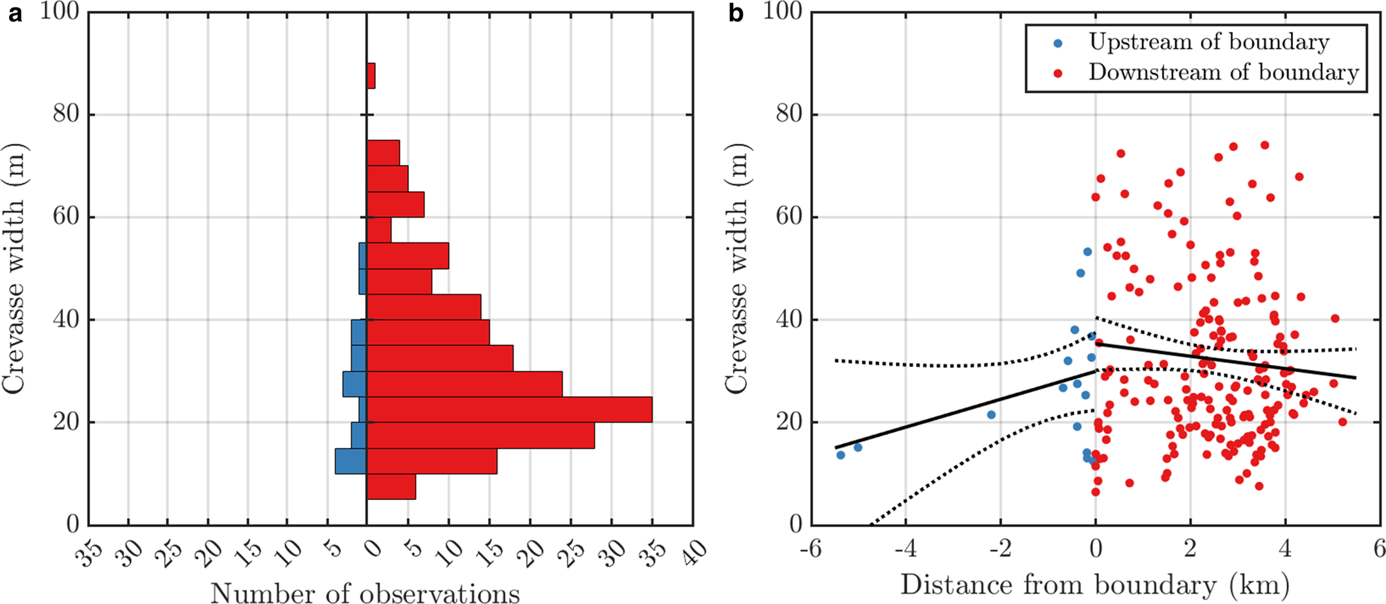
Figure 8. Observed widths of the 211 high-confidence crevasses. (A) Histograms of the calculated widths of ‘likely crevasses’, sorted by inside the firn aquifer (left histogram, blue) and outside the firn aquifer (right histogram, red), as in Figure 7. (B) Scatter plot of the calculated crevasse width versus the distance from the downglacier boundary of the firn aquifer, also sorted by inside the firn aquifer (negative distances; blue) and outside the firn aquifer (positive distances, red). Inside the firn aquifer (16 crevasses), crevasse width increases toward the boundary, but not significantly (p = 0.12). Outside the firn aquifer (195 crevasses), crevasse width peaks near the boundary and decreases downglacier, also not significantly (p=0.17). Black lines show the fitted trends and dashed lines show their 95% uncertainty bounds.
Next, we investigate trends in crevasse width with distance from the boundary. Inside the firn aquifer, crevasse width increases toward the boundary at a rate of 3 meters per kilometer, but this trend is not significant (p = 0.12). Crevasse width peaks at the boundary and, outside the boundary, decreases downglacier at a rate of 1.3 meters per kilometer; this trend is also not significant (p = 0.17). These trends and their uncertainty bounds are shown in Figure 8b.
Our crevasse detections span a ~10 km reach across the firn-aquifer boundary, as shown in Figure 8b. For the median ice flow speed of ~500 m a−1 at all crevasse locations (Joughin and others, Reference Joughin, Smith, Howat and Scambos2016, Reference Joughin, SMITH and HOWAT2018), this distance amounts to ~20 years of ice flow. Because the OIB flightlines that cross the firn-aquifer boundary are approximately parallel to ice flow, we capture a ~20 year history of crevasse width evolution in our data, summarized in Figure 8b.
4. Discussion
We discuss the limitations of our study and the implications of our finding that the firn aquifer primarily discharges through crevasses in our study area.
4.1 Implications of crevasse width data
The trends in crevasse width are not significant (p > 0.1): the slopes are not confidently different from zero (Fig. 8). This prevents us from making a firm conclusion, but we note that the most likely trends manifest in the directions consistent with our hypothesis that firn-aquifer water enters the crevasses at its downglacier boundary and widens them (p = 0.12, or 88% confidence); over time, each crevasse flows away from the firn aquifer and loses its water source, causing it to narrow (p = 0.17, or 83% confidence). We describe this conceptual model in more detail next.
Crevasses initially form at the ice-sheet surface, above the water table, as illustrated in Figure 1a. As limited local meltwater fills them, the crevasses deepen; if they reach the water table at a few tens of meters depth, firn-aquifer water flows in and enlarges them (Poinar and others, Reference Poinar2017). Contact with the water table is sufficient to establish density-driven hydrofracture, as water that flows into the crevasse will concentrate at the crack tip, forcing it ever deeper as long as new water flows in to maintain the pressure difference (Weertman, Reference Weertman1973; Alley and others, Reference Alley, Dupont, Parizek and Anandakrishnan2005; Krawczynski and others, Reference Krawczynski, Behn, Das and Joughin2009). Crevasses that have been in contact with the firn aquifer for longer – i.e., older crevasses that have flowed farther downstream – should contain more water and thus will be wider and deeper (Weertman, Reference Weertman1996). Our data for crevasse width inside the firn aquifer (blue dots in Fig. 8b) are consistent with this idea, but at a confidence level (p = 0.12) below what would be needed to conclude this definitively.
Over time, the crevasses flow downstream and lose contact with the firn-aquifer water, likely because a newly formed crevasse farther upglacier intercepts the water source (Fig. 1a). Once this occurs, we expect the original crevasse to narrow over time for at least three reasons: (1) Water slowly refreezes within the ice and is no longer replaced by the firn aquifer. (2) Water is more dense than ice and will tend to hydrofracture the crevasse to greater depths; to conserve water mass, the crevasse must narrow as it deepens. (3) Crevasses tend to open in areas of extensional stress and narrow as they flow into more compressional environments. While the third phenomenon is true of any crevasse, the first two are unique to crevasses with a water source (e.g., Weertman, Reference Weertman1996; Krawczynski and others, Reference Krawczynski, Behn, Das and Joughin2009). Thus, our data for crevasse width downglacier of the firn aquifer (red dots in Fig. 8b) also generally agree with a hydrofracture scenario, but at an insufficient confidence level (p = 0.17) to draw a firm conclusion.
Overall, our crevasse width data (Fig. 8) are consistent with but cannot fully support the conceptual model that water enters crevasses near the downglacier boundary of the firn aquifer and widens them, and as the ice continues to flow downstream, the crevasses become cut off from the firn aquifer water source and close up over a period of some years to decades.
4.2 Study limitations
4.2.1 Sampling bias within the study area
Our 29,000 km2 study area contains ~1500 linear kilometers of firn-aquifer boundary, roughly half of which is the downglacier boundary that we analyze. The OIB flightlines that we study cross this boundary 25 times, and the ATM instrument onboard the OIB aircraft has an across-track swath width of ~300 m. Thus, we directly sample only ~7.5 km, or ~0.1%, of the total firn-aquifer boundary across our study area.
The OIB flightlines were designed to provide representative observations of the ice sheet and its outlet glaciers (MacGregor and others, Reference MacGregor2021). Thus, our study likely oversamples the regions upstream of outlet glaciers compared to regions upstream of slower-moving ice. Outlet glaciers and their onset regions tend to be more heavily crevassed than surrounding areas. Therefore, we deduce that our finding that firn-aquifer water at 80% (20 out of 25) of our sites drains into crevasses is an upper bound on the true regional figure, since we likely oversample crevasse-prone areas.
4.2.2 Crevasse widths
Our methods observe only a fraction of the crevasses across our Southeast Greenland study area (Sect. 4.2.1). Although we ran our tool on every portion of the OIB flight lines within 10 km of a firn aquifer, there are nonetheless many more crevasses that went unsampled by OIB. Because OIB tends to prioritize dynamic environments ice-flow environments that are favorable to producing large crevasses, we deduce that this creates a weak positive bias in our crevasse width dataset.
Our restriction of sampling along OIB flight lines also, however, likely biases our crevasse widths as too-narrow for two reasons. First, the width of a crevasse varies along its length: like most edge cracks, crevasses are typically widest in their centers and taper to points on either end (Weertman, Reference Weertman1996). Ideally, we would measure the widest center part, but it is unrealistic to think that the flightlines cross every crevasse in their centers; instead, many undoubtedly intersect the narrower ends, making our widths overall too narrow. Second, the detection threshold of our tool is ≥2 m length or width (Sect. 2.3.1), and in an effort to reduce false positives, we farther reject any crevasses smaller than 1000 m2 (Sect. 2.3.2). These effects both bias the population too narrow.
Finally, limitations of our algorithm tend to introduce a widening bias. Figure 5 shows that for some crevasses, the ABCDE tool can only approximate their shape and size. In particular, the ABCDE tool does not always succeed in isolating the deep linear crevasse from more shallow recessed terrain around it. The centermost feature in Figure 5a is a good example: a high-confidence crevasse detection whose width we calculate as 21.5 m, whereas the widths of the surrounding crevasses, and of the southernmost portion of this detection, is closer to 10 m. In that image, the cause of this miscalculation may be regional snow accumulation that dampens the topography of the crevasse in this early April data. At other locations, such width overestimates are likely due to local sastrugi, which raise the average elevation of the reach/span and, therefore, make the true ice-sheet surface appear as a low anomaly in some places. Figure 5b shows such an example; however, these are crevasse-related features and, as such, their widths are discarded.
Overall, our crevasse widths are likely upper bounds. This may partially explain why we find a median crevasse width, 27 m, that is on the highest end of the range found by Poinar and others (Reference Poinar2017), 5–30 m, in the Helheim Glacier study area. Our median is higher than 88% of the crevasses identified in optical imagery by Poinar and others (Reference Poinar2017) in that limited area.
4.2.3 Identification of the downglacier boundary of the firn aquifer
Miége and others (Reference Miége2016) analyzed two OIB radars of different frequencies to identify the firn-aquifer water table and its spatial extent. These were the accumulation radar, a 565–885 MHz radar with a center wavelength of 40 cm that penetrates 60–80 m below the ice-sheet surface, and the Multi-Channel Coherent Radar Depth Sounder (MCoRDS) radar, a 180–210 MHz radar with a center wavelength of 1.5 m that penetrates multiple kilometers through the ice to sense the ice-sheet bed. The shorter wavelength of the accumulation radar allows it to resolve the water table, which manifests in radargrams as a linear, dark absorber surface. However, near-surface features such as crevasses can interfere with this signal, sometimes obscuring the water table below. Given that we detect crevasses at 80% of the downglacier boundaries of the firn aquifer, it is reasonable to question whether the Miége and others (Reference Miége2016) boundary is truly the end of the firn aquifer, or if instead near-surface crevasses prohibit the radar from detecting the water table. This scenario is, incidentally, illustrated in the left-most part of Figure 1a.
Miége and others (Reference Miége2016) use the MCoRDS radar to counter this interference. In the absence of a firn aquifer, the long-wavelength MCoRDS radar penetrates through the full ice thickness and provides a clear, coherent bed return, regardless of shorter-lengthscale ice surface features such as crevasses. Englacial water, however, absorbs the radar energy and blocks it from reaching and reflecting off the bed. This manifests as the absence of a bed reflector in the MCoRDS data; Miége and others (Reference Miége2016) interpreted a missing bed echo as evidence of a firn aquifer. Thus, regardless of any expected interference of crevasses with the accumulation radar signal, the Miége and others (Reference Miége2016) aquifer boundaries accurately reflect the extent of the water table.
The Miége and others (Reference Miége2016) data for firn-aquifer extent reflects all OIB observations collected over 2010–2014; however, we study crevasses only in 2013. The extent of the firn aquifers we use is therefore an upper bound on the 2013 extent. Thus, the true downglacier boundary in 2013 may be a few kilometers inland from where the Miége and others (Reference Miége2016) data indicate. This systematic error could cause the true zero point of our distances in Figures 7–8 to be farther left (inland) than indicated. A 2 km error, for instance, would mean that up to 58 of the 92 of crevasses we detected inside the firn aquifer (63%) are in fact outside it, where they would likely be draining water.
Finally, Miége and others (Reference Miége2016) and Miller and others (Reference Miller2020) found that spatial limits of the firn aquifer change over time. At two well-studied sites near Helheim Glacier, the downglacier boundary has fluctuated by 1–2 km over 2010–2017, without a trend. These fluctuations are within the few-kilometer bias discussed above, so we do not treat them separately. The inland limit at these locations has expanded by 5–7 km over the same period. This is likely in response to increased melt at higher elevations in recent decades; however, in this work, we do not study the inland boundary.
4.3 Fate of the firn-aquifer water
Over the period 2010–2017, the water table at two well-studied Helheim Glacier sites has been rising inland and sinking near (within 5–10 km) the downglacier boundary (Miller and others, Reference Miller2020). The rising implies increased melt rates in the catchment; e.g., the high melt summers of 2010 and 2012 (Hanna and others, Reference Hanna2021) were followed by observations of higher water tables in the springs of 2011 and 2013 (Miége and others, Reference Miége2016). The sinking, which is non-monotonic in time, implies time-variable flow out of the aquifer (Miller and others, Reference Miller2017a). This would be inconsistent with the hypothesis that water leaves the aquifer only by refreezing at its bottom (Fig. 1c), as refreezing rates are controlled by the vertical temperature gradient some 30 m below the ice-sheet surface and thus should be steady in time (Meyer and Hewitt, Reference Meyer and Hewitt2017; Montgomery and others, Reference Montgomery2017; Miller and others, Reference Miller2020). Similarly, a sinking water table is also inconsistent with discharge into near-surface springs (Fig. 1b), which are anyway not observed in this area (Dunmire and others, Reference Dunmire, Banwell, Wever, Lenaerts and Datta2021). It is, however, consistent with time-variable discharge into crevasses (Fig. 1a). The aquifer-water-fed crevasse may slowly deepen to the full thickness and connect to the subglacial environment, as modeled by Poinar and others (Reference Poinar2017) and McNerney (Reference McNerney2016), or it may arrest partway. A full-thickness crevasse would continually drain aquifer water through the basal environment to the ocean; similarly, a crevasse that attenuated englacially could also continually drain aquifer water as it hydrofractured downward and refroze the water englacially. Either type of crevasse could potentially drain the aquifer at a greater rate than meltwater could recharge it; this would lower the water table.
Our results and the water table observations do not by themselves constrain whether the water-filled crevasses reach the bed or, alternately, carry the water deep inside the ice sheet to refreeze. Modeling work constrained by known water fluxes through the Helheim Glacier firn aquifer shows that any crevasses fed by local firn-aquifer water are likely to be driven to the bed, rather than arresting part way (McNerney, Reference McNerney2016; Poinar and others, Reference Poinar2017). While in situ measurements of water flux are not available for most of our study sites, the fluxes are a function of melt rate, firn temperature and porosity, and surface slope (Miller and others, Reference Miller2017a). We examine these across our study area in turn. The climatology is not greatly variable in space, which implies similarity in melt rates and firn temperature across our study area (Fettweis and others, Reference Fettweis2020). Next, large-scale surface slopes vary by as much as a factor of two over our study area, from ~0.015 to ~0.03 (Howat and others, Reference Howat, Negrete and Smith2014, Reference Howat, Negrete and Smith2022). Finally, spatial variations in the porosity of the firn are not well constrained (Miller and others, Reference Miller2017a), but porosity varies by $\sim 30\%$ vertically at the Helheim Glacier site (Koenig and others, Reference Koenig, Miége, Forster and Brucker2013), and field measurements in West Greenland suggest horizontal spatial variations of some 20–30% (Clerx and others, Reference Clerx2022). Considering these four factors together, we estimate that water fluxes through the firn aquifer may differ by up to a factor of three from the Helheim Glacier site. This is well within the range tested by Poinar and others (Reference Poinar2017) that resulted in propagation to the glacier bed.
Given the widths of the crevasses at the surface, we can indirectly estimate their depths through the width-to-depth aspect ratio of a fracture, which should be roughly equivalent to the ratio of surface deviatoric stress and the shear modulus of the material (Trunz and others, Reference Trunz2022). An estimated shear modulus of ~1 GPa for ice and ~0.01 GPa for firn (Sigrist, Reference Sigrist2006) and surface deviatoric stresses ≤10 − 100 kPa yields a width-to-depth ratio range of 10−5 − 10−2. We found a median crevasse width of 27 m at the downglacier boundary of firn aquifers in our study area; this implies a propagation depth of at least ~3000 m, which is substantially greater than the ~700–1000 m ice thickness in our study area (Morlighem and others, Reference Morlighem2017; Morlighem, Reference Morlighem2021). As noted above, however, our observed crevasse widths are upper bounds, so they do not provide unambiguous evidence of drainage to the bed. If we have overestimated the crevasse widths by a factor of two, these widths are likely still consistent with full-thickness fractures. If we have overestimated by more than that, it may be that the water in the crevasses does not reach the bed, but refreezes inside the ice sheet (Lüthi and others, Reference Lüthi2015; Poinar and others, Reference Poinar, Joughin, Lenaerts and van den Broeke2016). In West Greenland, Kendrick and others (Reference Kendrick2018) inferred similar behavior: propagation of a water-filled crevasse to ~50 m depth during the melt season, then slow refreezing over the next year. There were no firn aquifers in that area to concentrate the meltwater.
4.4 Potential effects on ice dynamics
Above, we identified two possible fates for firn-aquifer water that discharges into crevasses: (1) the crevasse carries it to the ice-sheet bed, or (2) propagation of the crevasse stops and the water refreezes within the ice sheet. Both scenarios affect the local and regional flow of the ice sheet and thus ice-sheet mass balance and global sea levels. We address the effects on ice flow of each mechanism on ice flow in turn.
First, the downglacier boundary of the firn aquifer, and the crevasses the firn aquifer feeds, sit at ~1500 m elevation across our study area (Miége and others, Reference Miége2016; Howat and others, Reference Howat, Negrete and Smith2022). The bare-ice zone, where large volumes of surface meltwater reach the bed over the melt season, begins at ~1000 m elevation (Fettweis and others, Reference Fettweis2020; Howat and others, Reference Howat, Negrete and Smith2022). This 500 m elevation difference translates to ~10–40 km horizontally, given regional surface slopes of ~0.015 to ~0.03 (Howat and others, Reference Howat, Negrete and Smith2022). Thus, if the crevasses carry the firn-aquifer water to the bed, the water reaches the subglacial environment ~10–40 km farther inland than it would without the firn-aquifer – crevasse system. Poinar and others (Reference Poinar, Dow and Andrews2019) modeled a hypothetical firn-aquifer–crevasse system that drained to the bed across a similar geometry and found that the aquifer water had an outsized effect on the basal hydrologic system. The inland water source kept the subglacial system in its channelized, efficient state for a longer period each year. Such subglacial conditioning would stabilize seasonal fluctuations in glacier speed in a way that is consistent with observations on outlet glaciers across our study area (Moon and others, Reference Moon2014).
Second, we address firn-aquifer water that refreezes in crevasses without reaching the bed. This water may penetrate tens to hundreds of meters depth, but comes short of the 700–1000 m required to reach the bed in our study area. Basic thermodynamic principles, supported by observations in West Greenland, stipulate that this water will refreeze over a period of decades to centuries, depending on the ambient deep ice temperature and the width of the crevasse (Thomsen, Reference Thomsen1988; Phillips and others, Reference Phillips, Rajaram and Steffen2010; Lüthi and others, Reference Lüthi2015; Poinar and others, Reference Poinar, Joughin, Lenaerts and van den Broeke2016). The refreezing transfers latent heat into the ice, warming it and decreasing its viscosity, making the local ice flow faster (Phillips and others, Reference Phillips, Rajaram and Steffen2010). At the well-studied Helheim Glacier site, Poinar and others (Reference Poinar2017) calculated that such latent heat transfer would increase ice flow speeds by roughly 5–30% over a ten-year period. Field measurements indicate that the aquifer there is 15–60 years old (Miller and others, Reference Miller2020); if crevasses have been draining the aquifer for its whole lifetime, then the deformation estimates are a lower bound. For similar ice temperature, driving stress and ice thickness, we expect similar modest increases in ice flow speed across our study sites.
Overall, the aquifer water would have a much greater effect on ice flow speed, and thus on ice-sheet mass balance, if it reaches the glacier bed (Culberg and others, Reference Culberg, Chu and Schroeder2022). Our measured crevasse widths are consistent with the hypothesis that firn-aquifer water may drain to the bed at many (up to 80%) of our study sites (Poinar and others, Reference Poinar2017) but cannot significantly support it. More detailed research is needed to better constrain the depths that these crevasses carry the water, including whether they reach the bed. These research needs include, as a top priority, measurements of horizontal water flux through firn aquifers across our study area, similar to those obtained by Miller and others (Reference Miller2017a) near Helheim Glacier, and secondarily, additional ice-sheet-wide surveys of crevasse width, similar to the limited analysis of the 2013 OIB data we performed here. Such new surveys may be enabled by high-resolution altimetry data currently being collected by ICESat-2 (Markus and others, Reference Markus2017).
5. Conclusion
Over the past decade, the community has made significant advances in understanding the role of firn aquifers on surface mass balance across the Greenland Ice Sheet. More recently, their connection to the subglacial system has been studied at one field site near Helheim Glacier, where model-based analysis showed that the firn-aquifer water could fundamentally change the seasonal evolution of the subglacial water system that modulates ice motion. Thus, the full effect of firn aquifers on ice-sheet mass balance is a new frontier. We find that the most likely fate of firn aquifer water over the sites we studied in Southeast Greenland is drainage through crevasses, which occurred at 80% of (20 of 25) sites. It is likely, but not fully constrained by our work, that these crevasses carry the firn-aquifer water to the glacier bed, from where it has a clear path to the ocean. At the other 20% of sites, the firn-aquifer water stays near the surface, either refreezing at tens of meters depth or re-emerging at the surface and running off into downglacier firn, where it refreezes in the top 5–10 meters. Our results imply that the liquid water contained in a large fraction of the firn aquifers in Southeast Greenland may reach the ocean, although recharge from ongoing surface melt refills and maintains the aquifers.
Data
All data produced by this research and presented in this manuscript are publicly available at ubir.buffalo.edu/xmlui/handle/10477/84554. All code used for this analysis is available for free use (after user registration) at theghub.org/resources?alias=crevasseoib (Jones-Ivey and others, Reference Jones-Ivey, Sperhac and Poinar2021).
Acknowledgements
This research was funded by the U.S. National Science Foundation (NSF) grant number 2004302, ‘Ghub as a Community-Driven Data-Model Framework for Ice-Sheet Science.’ Computing resources for this work were supplied and supported by the University at Buffalo's Center for Computational Research (CCR). We thank the entire Ghub scientific team, including Erika Simon, Sophie Nowicki, Justin Quinn, Eric Larour, Beata Csatho, William Lipscomb, Denis Felikson, Isabel Nias and Elliot Snitzer.


 Open access