


I. INTRODUCTION
The problem of estimating covariance matrices often appears in signal processing and multivariate analysis. Thus, the estimation accuracy of the covariance matrices is important in signal processing, in general. The estimation accuracy depends on the estimator. The most popular one is the sample covariance matrix and it is equivalent to the maximum likelihood estimator (MLE) under the Gaussian assumption. The MLE has good properties such as asymptotic unbiasedness, consistency, and asymptotic efficiency, but these apply only for big data. The MLE does not perform well when the dataset is small. Another case of failure in MLE is when some eigenvalues take the same or almost same values. For the identity matrix, e.g., the eigenvalues of the sample covariance matrix are spread out [Reference Johnstone1]. This problem is not rare. In fact, the subspace methods for system identification assume the covariance matrix is the sum of a low-rank matrix for signals and the identity matrix for noises, which leads to this kind of matrix [Reference Katayama2]. Another case is the spike-and-slab prior distribution in Bayesian model selection [Reference Ishwaran and Rao3]. Thus, it is important to elucidate the mechanism of the degradation in estimating duplicated eigenvalues especially for a small dataset.
One approach to tackle the problem of duplicated eigenvalues is shrinkage estimation methods [Reference Bickel and Levina4–Reference Ledoit7]. Donoho et al. proposed an estimator that is optimal for the spiked covariance matrix, i.e., all the eigenvalues of the population matrix are equal except the maximum one [Reference Donoho, Gavish and Johnstone8]. They gave the risk of estimation called Stein's loss [Reference James and Stein9] as a function of the maximum eigenvalue using random matrix theory [Reference Baik, Ben, Arousa and Peche10]. Their result shows the optimal estimator  $\hat {\Sigma }= \hbox{diag}(\hat {\lambda _{1}},1,1,\ldots )$ for the population covariance is $\Sigma = \hbox{diag}(\lambda _{1},1,1,\ldots )$ is expressed as
 $$\hat{\lambda}_{1} = \left\{\matrix{\displaystyle{\ell_{1} \over \alpha + \left(1 - \alpha \right)\ell_{1}} \hfill & {\rm if}\ \ell_{1} \gt \left(1 + \sqrt{\gamma} \right)^{2}, \hfill \cr 1 \hfill & {\rm otherwise}, \hfill} \right.$$
where
 $$\alpha =\displaystyle{1-({\gamma})/({\left(\ell_{1}-1\right)^{2}}) \over 1+({\gamma})/({\ell_{1}-1})},$$
γ is the ratio of the number of variables to that of observations, and ℓ1 is the maximum eigenvalue of the sample covariance matrix expressed as
 $$\ell_{1} = \left\{\matrix{\lambda_{1} \left(1 + \gamma/\left(\lambda_{1} - 1\right) \right) \hfill & {\rm if} \lambda_{1} \gt 1 + \sqrt{\gamma}, \hfill \cr \left(1 + \sqrt{\gamma} \right)^{2} \hfill &{\rm otherwise}. \hfill} \right.$$
The result shows the risk of estimation,  $L(\Sigma , \hat \Sigma )$, increases as λ 1 increases, until the maximum eigenvalue reaches the transition point and then it decreases to zero thereafter. This means the risk is a non-monotonic function of λ 1 (Fig. 1).

Fig. 1. Risk of estimation vs. the maximum eigenvalue (γ = 1/4).
Although this property of non-monotonicity is interesting, the theoretical results hold only in the asymptotic that both the numbers of variables and observations go to infinity. As seen in the MLE case, finite variables and/or observations change the performance. Thus, an analysis of the risk in more realistic cases is necessary.
The problem of finite observations is formulated as the learning curve in machine learning, which is the averaged generalization/prediction error as a function of the number of observations [Reference Amari, Fujita and Shinomoto11]. In Bayesian statistics, the learning curve is expressed as the learning coefficient divided by the number of observations. That is, the learning coefficient is defined as the coefficient of the leading term of the mean Kullback–Leibler divergence from the true to predicted distributions [Reference Watanabe12,Reference Watanabe and Amari13]. When the probability model is parametric and regular, i.e., uniquely identifiable, the learning coefficient is represented as a half of the number of the parameters. When the model is singular, however, the learning coefficient takes a smaller value than a half of the number of parameters, depending on the probability model. This idea is applicable to the estimation of covariance matrices with duplicated eigenvalues since this is a singular model due to the duplication of eigenvalues and unidentifiable eigenvectors associated with them [Reference Sheena14].
The learning coefficient of a singular model is, however, difficult to derive in general and, only several special cases have been solved so far [Reference Yamazaki and Watanabe15–Reference Watanabe and Watanabe18]. Thus, to give an exact analysis to a finite case, we considered a specific algorithm, a shrinkage method based on the empirical Bayes method, and derived its learning coefficient in a simple case of two dimensions. As a result, the learning coefficient of the algorithm has a non-monotonic property with respect to the maximum eigenvalue of the population covariance matrices in the same way as the infinite case, although the methods for these analyses are totally different. Finally, we confirmed the theoretical value through numerical experiments.
II. PRELIMINARIES
Let X i(i = 1, …, N) be D-dimensional vectors independently drawn from an identical normal distribution with mean 0 and covariance Σ and
 $$S = \displaystyle{1 \over N} \sum_{i=1}^{N}X_{i}X_{i}^{T},$$
the sample covariance matrix, respectively. Then, Σ and S are diagonalized using orthogonal matrices V and U as
 $$\Lambda = \hbox{diag}\left(\lambda_{1},\ldots,\lambda_{D}\right) = V^T \Sigma V,$$
 $$L = \hbox{diag}\left(\ell_{1},\ldots,\ell_{D}\right) = U^T S U,$$
where λ 1 ≥ · · · ≥ λ D and ℓ1 ≥ · · · ≥ ℓD are the eigenvalues of Σ and S and  $\hbox{diag}(\cdot)$ denotes the diagonal matrix of ·. Note since the sample covariance matrix S and its eigenvalues L are sufficient statistics of the covariance matrix Σ and its eigenvalues Λ, estimators of Σ and Λ are written as $\hat{\Sigma}(S)$ and $\hat{\Lambda}(L)$, respectively, where $\hat{\Lambda} = \hbox{diag}(\hat{\lambda}_{1}, \ldots, \hat{\lambda}_{N})$.
Let us consider a shrinkage method that can explicitly treat duplication of eigenvalues. Since duplication of eigenvalues makes eigenvectors unidentifiable uniquely, we concentrate on the estimation of eigenvalues irrespective of eigenvectors. This is useful even when eigenvectors are desired because they can be calculated taking the duplication into account. For this purpose, we introduce a hierarchical model where V is chosen from the uniform distribution on the orthogonal matrix space with fixed Λ, i.e.,
 $$X_{i} \sim{\cal N}(0,V\Lambda V^{T}), \quad V \sim p\left(V\vert \Lambda \right),$$
and consider a Bayesian estimation method. Note it is natural to consider eigenvalues and eigenvectors separately when treat duplicated or repeated eigenvalues since the latter are not identifiable [Reference Kenny and Hou19]. The joint distribution of S and V for this model is written as
 $$\eqalign{p\left(S,V\vert N,\Lambda\right) &= p\left(L,U,V\vert N,\Lambda\right) \cr &=p\left(L,U\vert N,V,\Lambda\right)p\left(V\vert \Lambda\right).}$$
Here, p(L, U|N, V, Λ) is the joint probability of the eigenvalues and their eigenvectors of sample covariance matrix, which is obtained by transforming the Wishart distribution with degree of freedom N and the scale matrix VΛV T. An important property of this model is the support of the distribution of covariance matrix, p(Σ) = p(VΛV T), varies depending on the hyperparameters Λ. For example, when Λ is the identity matrix, Σ is also the identity matrix irrespective of V .
A popular method to determine the hyperparameters Λ is the empirical Bayes method. We calculate the marginalized likelihood by integrating p(L, U|N, V, Λ)p(V|Λ) over the orthogonal matrix space and maximize it, i.e.,
 $$\hat{\Lambda}\left(L\right) =\mathop{\hbox{argmax}}\limits_{\Lambda}p\left(S\vert \Lambda\right)$$
 $$=\mathop{\hbox{argmax}}\limits_{\Lambda}\int p\left(L,U\vert N,V,\Lambda\right)p\left(V\vert \Lambda\right)dV.$$
Since this integration is invariant under any orthogonal transformation  $S \mapsto VSV^{T} $, the distribution of V can be replaced with the Haar measure on the orthogonal matrix space [Reference Braun20]. Then, the marginal likelihood is expressed using hypergeometric function with matrix argument [Reference James21]. Since the marginal likelihood is difficult to maximize due to the complexity of the hypergeometric function, in general, we only consider a special case of the spiked covariance model for Σ, i.e., λ 1 ≥ λ 2 = λ 3 = · · · = λ D [Reference Johnstone1]. In addition, we use the eigenvectors of the sample covariance matrix for the estimation instead of the posterior p(V|S), i.e., $\hat{\Sigma} = U \hat{\Lambda} U^{T}$, which is often supposed in the shrinkage estimation.
Note although the learning coefficient is originally defined for Bayesian estimation, it makes sense since shrinkage estimation can be regarded as an approximation of the posterior in hierarchical models [Reference Nakajima and Watanabe22].
III. MAIN RESULTS
We show some facts on the shrinkage estimation with our hierarchical model before deriving the learning coefficient of the proposed estimation method. See Appendix for the proofs.
Proposition 1
For the marginal likelihood of the hierarchical model (7) with spiked covariance model, the following statements hold.
(i) The marginal likelihood is written as
where 1F 1 denotes the hypergeometric function with matrix argument [Reference Magnus and Oberhettinger23]. $$\eqalign{p\left(S\vert \Lambda\right) & =\int p\left(L,U\vert N,V,\Lambda\right)p\left(V\vert \Lambda\right)dV \cr & \propto\left\vert \Lambda\right\vert ^{-{N}/{2}}\exp\left[-\displaystyle{N \over 2}\lambda_{2}^{-1}\hbox{tr} S\right] \cr & \quad \cdot {}_{1}F_{1} \left(\displaystyle{1 \over 2};\displaystyle{D \over 2};\displaystyle{N \over 2}\left(\lambda_{2}^{-1}-\lambda_{1}^{-1}\right)S\right)}$$
(ii)
$\Lambda = \hbox{diag}(\lambda _{1},\lambda _{2},\ldots ,\lambda _{2})$ that maximizes p(S|Λ) satisfies the following equations,
(11)$$\hbox{tr}\Lambda =\lambda_{1}+\left(D-1\right)\lambda_{2} =\hbox{tr} S,$$(12)where F(z) = 1F 1(1/2;D/2;zS) and F′(z) is its derivative.$$\lambda_{1} =\displaystyle{1 \over N}\displaystyle{F' \left({N}/{2}\left(\lambda_{2}^{-1}-\lambda_{1}^{-1}\right)\right) \over F\left({N}/{2}\left(\lambda_{2}^{-1}-\lambda_{1}^{-1}\right)\right)},$$(iii) If there exists a non-trivial solution of the equations above, it maximizes the marginal likelihood, where the trivial solution is
$\lambda _{1}=\lambda _{2}=\hbox{tr} S/D$.(iv) The equations have a non-trivial solution if and only if
(13)$$ND\sum_{i \lt j}(\ell_{i}-\ell_{j})^{2}-(D^{2}+D-2)(\hbox{tr} S)^{2} \gt 0.$$


In the two-dimensional case, the marginal likelihood is explicitly calculated.
Corollary 2
When D=2, the marginal likelihood is given by
 $$\eqalign{p(S\vert \Lambda) & =\displaystyle{N^{N}\left(\ell_{1}-\ell_{2}\right)\left(\ell_{1}\ell_{2}\right)^{({N-3})/{2}}\left(\lambda_{1}\lambda_{2}\right)^{-{N}/{2}} \over 4\Gamma\left(N-1\right)}\cr & \quad\cdot \exp\left[-\displaystyle{N\left(\ell_{1}+\ell_{2}\right)\left(\lambda_{1}+\lambda_{2}\right) \over 4\lambda_{1}\lambda_{2}}\right] \cr & \quad\cdot I_{0}\left(\displaystyle{N\left(\ell_{1}-\ell_{2}\right)\left(\lambda_{1}-\lambda_{2}\right) \over 4\lambda_{1}\lambda_{2}}\right),}$$
where I k(z) denotes the modified Bessel function of the first kind with order k.
Since  $\int p(S\vert \Lambda )d\ell _{1}d\ell _{2}=1$ holds, (14) can be regarded as the joint probability density function of the eigenvalues of the sample covariance matrix with respect to ℓ1, ℓ2. By substituting D=2 into Proposition 1, the estimator of eigenvalues is given explicitly.
Corollary 3
The estimator that maximizes (14) is given by
 $$(\hat{\lambda}_{1},\hat{\lambda}_{2}) = \left\{\matrix{\left(\displaystyle{\ell_{1}+\ell_{2} \over 2},\displaystyle{\ell_{1}+\ell_{2} \over 2}\right), \hfill & {\rm if } \left(\displaystyle{\ell_{1} \over \ell_{2}}-1\right)N^{1/2} \hfill \cr &\lt 2^{3/2}\left(\!1+\displaystyle{\sqrt{2}N^{1/2}+2 \over N-2}\!\right), \hfill \cr \left(\displaystyle{\ell_{1}+\ell_{2}+t \over 2},\displaystyle{\ell_{1}+\ell_{2}-t \over 2}\right), \hfill & {\rm otherwise}, \hfill}\right.$$
where t is the solution of
 $$t = \left(\ell_{1}-\ell_{2}\right)A\left(\displaystyle{N\left(\ell_{1}-\ell_{2}\right)t \over \left(\ell_{1}+\ell_{2}\right)^{2}-t^{2}}\right)$$
and A(z) = I 1(z)/I 0(z).
Corollary 3 gives the relation between the eigenvalues of the sample covariance matrix and the estimated eigenvalues by our shrinkage estimation (Fig. 2). When the two eigenvalues l 1 and l 2 are closer together than a threshold, the estimators of  $\hat {\lambda }_1$ and $\hat {\lambda }_2$ take the same value.
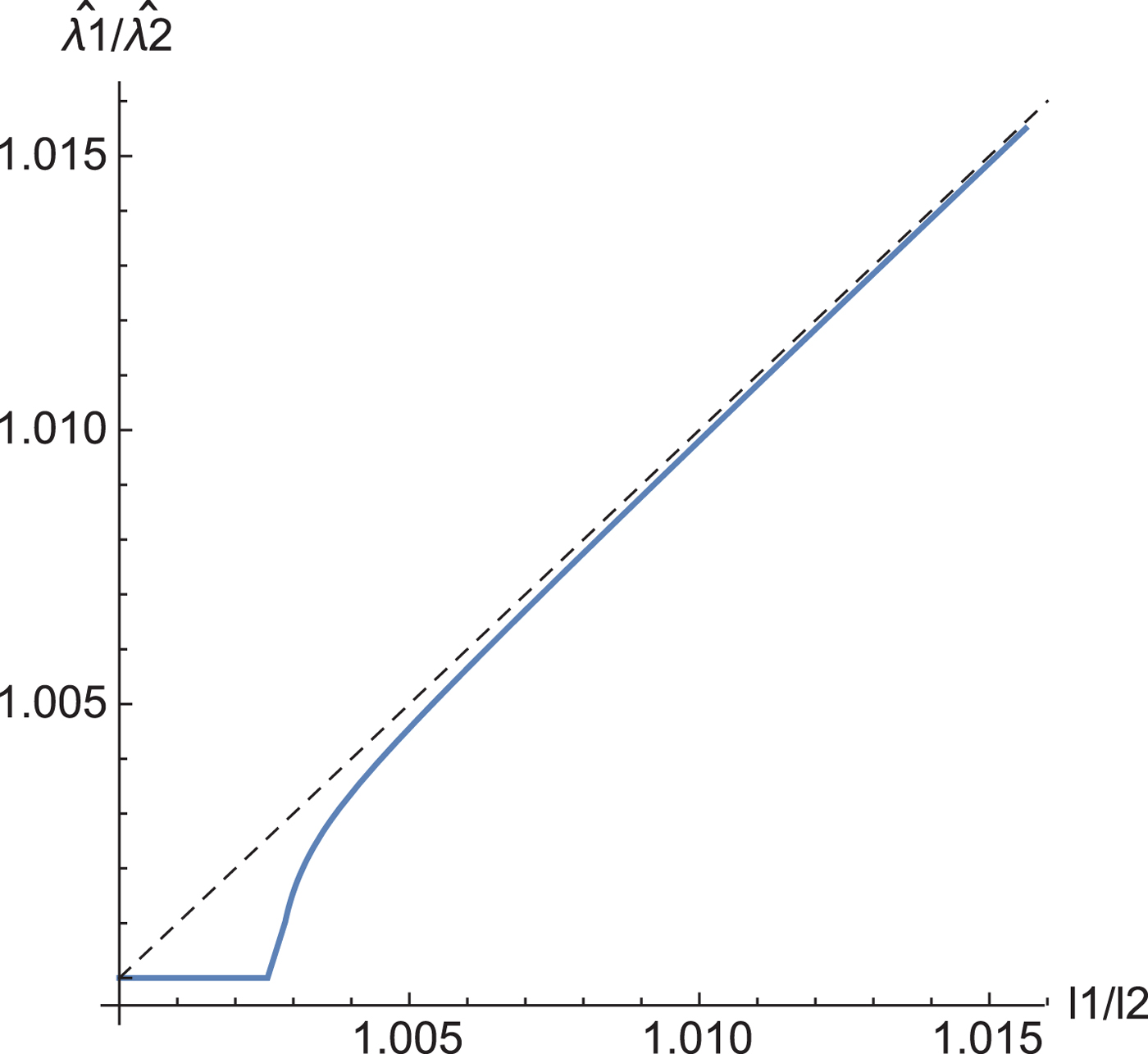
Fig. 2. The relation between the eigenvalues of the sample covariance matrix and those of the estimated eigenvalues. N = 220.
A) Derivation of learning coefficient
The learning coefficient is defined based on the Kullback–Leibler divergence [Reference Watanabe12]. The mean of the Kullback–Leibler divergence from the true distribution p to the predicted one q is called the Bayesian generalization error in asymptotics, which is written as
 $$ E\left[\hbox{KL}\left(p\vert \vert q\right)\right] =\displaystyle{\kappa \over N}+o\left(\displaystyle{1 \over N}\right), $$
where E[ · ] denotes the expectation with respect to the observations. The coefficient of leading term κ is called the learning coefficient. In case that the distributions are D-dimensional multivariate normal distribution with mean 0 and covariance matrices Σ1 and Σ2, respectively, the Kullback–Leibler divergence is described as
 $$\hbox{KL}\left(\Sigma_{1}\vert \vert \Sigma_{2}\right) =\displaystyle{1 \over 2}\left(\hbox{tr}\Sigma_{1}^{-1}\Sigma_{2}-\log\Sigma_{1}^{-1}\Sigma_{2}-D\right),$$
which is equivalent to the Stein's loss of covariance matrices [Reference James and Stein9]. When a statistical model is regular, as a special case, its learning coefficient of maximum likelihood estimation becomes the half of the number of parameters [Reference Watanabe12], i.e.,
 $$ E\left[\hbox{KL}\left(\Sigma\vert \vert S\right)\right]N \simeq\displaystyle{D\left(D+1\right) \over 2},$$
when the estimator of the covariance matrix is the sample covariance matrix.
In our case, the expectation with respect to the observations X i(i = 1, …, N) is equivalent to the expectation with respect to the sample covariance matrix S. Thus, the learning coefficient for  $\hat{\Sigma} (S)$ is given by
 $$\eqalign{&E[\hbox{KL}(\Sigma\vert \vert \hat{\Sigma}(S))]N \cr & \simeq \displaystyle{D(D+1) \over 2}+E[\hbox{tr}\Sigma^{-1}(\hat{\Sigma}(S)-S)]N \cr &\quad -E[\log\vert S^{-1}\hat{\Sigma}(S)\vert ]N.}$$
Using the proposed shrinkage estimator of the covariance matrix,
 $$\hat{\Sigma}\left(S\right) = U \left[\matrix{\hat{\lambda}_{1} \hfill & \cr \hfill & \hat{\lambda}_{2} \hfill}\right]U^{T},$$
and the reparametrization as
 $$\matrix{\lambda =\lambda_{2} \hfill & c =\left(\lambda_{1}/\lambda_{2}-1\right)N^{1/2} \hfill \cr \ell =\ell_{2} d \hfill &=\left(\ell_{1}/\ell_{2}-1\right)N^{1/2} \hfill \cr e =t/\ell_{2}N^{1/2}, \hfill & \hfill}$$
the second and the third terms of (18) are given by
 $$\eqalign{&E[\hbox{tr}\Sigma^{-1}(\hat{\Sigma}-S)]N =\displaystyle{c \over 2}\lambda^{-1}(1+cN^{-1/2})^{-1} \cr & \quad\cdot E\left[(d-e)\ell\left(1-2\left(V_{11}^{2}+U_{11}^{2}\right)\right.\right. \cr &\qquad \left. \left. +\,4V_{11}U_{11}\left(V_{11}U_{11}+V_{12}U_{12}\right)\right)\right]}$$
 $$\simeq\displaystyle{c \over 2}A\left(\displaystyle{c^{2} \over 4}\right)E[d-e],$$
 $$\eqalign{&E[\log\vert S^{-1}\hat{\Sigma}\vert ]N \cr &= E\left[\log(1+dN^{-1/2})^{-1}\left(1+\displaystyle{d+e \over 2}N^{-1/2}\right) \right. \cr &\quad \cdot \left.\left(1+\displaystyle{d-e \over 2}N^{-1/2}\right)\right] \cr & \simeq \displaystyle{1 \over 4}E[d^{2}-e^{2}],}$$
respectively. Note that this kind of reparameterization is widely used in evaluating learning coefficients [Reference Watanabe and Amari13,Reference Nakajima and Watanabe22]. In (22) and (23), the difference between the eigenvalues of shrinkage estimator, e, and the probability density function of the distance of eigenvalues of the sample covariance matrices, d, can respectively be approximated to the solution of dI 1(de/4) − eI 0(de/4) = 0 and the solution of  $p(d)=\displaystyle{d \over 4} \exp [-({c^{2}+d^{2}})/{8}]I_{0}({cd}/{4})$. See Appendix for the validity of these approximations.
B) Numerical experiments
To validate the derived learning coefficient, some numerical experiments were carried out. The experimental learning coefficients were calculated as the Kullback–Leibler divergence from the true distribution to the predicted distribution averaged over 104 sample covariance matrices, multiplied by 2N, while the theoretical learning coefficients were numerically calculated using (18), (22), and (23). The two learning coefficients coincide well, including their non-monotonicity (Fig. 3).

Fig. 3. Learning coefficients versus c, the normalized eigenvalue ratio. Experiments (solid) and theory (dashed).
IV. DISCUSSION
How duplication of eigenvalues in covariance matrices affects estimation was clarified here. We derived the learning coefficient of a shrinkage estimator based on the empirical Bayes method where both the numbers of variables and observations are finite. Our shrinkage estimation method has two phases depending on the sample eigenvalues, i.e., in one phase the estimation error increases when the population covariance matrix has eigenvalues closer to each other than a threshold while in the other phase the learning coefficient varies smoothly with respect to the difference of eigenvalues. This phenomenon is consistent with an asymptotic case where the numbers of variables and observations are infinite. However, the influence of duplication is stochastic in the finite case and the state fluctuates between the two phases while the influence of duplication is deterministic in the infinite case. The analysis of the fluctuation is still open.
Our analysis treated the simple case of two-dimensional. To expand our results, we need to calculate the marginal likelihood in (8) for general cases. Although this is written using the generalized Bingham distribution or its product, the derivation of the estimators or the conditions is difficult due to the complexity of the hypergeometric function. We need a new method to solve this problem. Nonetheless, this work has given a new insight to this problem because the Bayesian approach is shown to be hopeful.
FINANCIAL SUPPORT
This work was supported by JSPS KAKENHI Grant Numbers 25280083, 17H01817, 17H05863.
STATEMENT OF INTEREST
None.
APPENDIX
Proof of Proposition 1
Since p(L, U|N, V, Λ) in (8) is the joint distribution of eigenvalues and eigenvectors transformed from the Wishart distribution with degree of freedom N and scale matrix VΛV T, the probability density function is given by
 $$\eqalign{& p\left(L,U\vert N,V,\Lambda\right)\cr & =\displaystyle{N^{ND/2}\left\vert S\right\vert ^{\left(N-D-1\right)/2}\exp\left(-\left(N/2\right){\rm tr}\left(SV\Lambda^{-1}V^{T}\right)\right) \over 2^{ND/2}\left\vert \Lambda\right\vert ^{N/2}\Gamma_{D}\left(N/2\right)} \cr & \quad\cdot \prod_{i \lt j}\left\vert \ell_{i}-\ell_{j}\right\vert} $$
 $$\eqalign{&=\displaystyle{N^{ND/2}\left\vert L\right\vert ^{\left(N-D-1\right)/2}\exp\!\left(-\left(N/2\right){\rm tr}\!\left(ULU^{T}V\Lambda^{-1}V^{T}\right)\!\right) \over 2^{ND/2}\left\vert \Lambda\right\vert ^{N/2}\Gamma_{D}\left(N/2\right)} \cr & \quad\cdot \prod_{i \lt j}\left\vert \ell_{i}-\ell_{j}\right\vert,} $$
where ΓD denotes the multivariate gamma function defined as
 $$\Gamma_{D}\left(N/2\right)= \pi^{D\left(D-1\right)/2} \prod_{i=1}^{D}\Gamma\left(\displaystyle{1 \over 2}\left(N-i+1\right)\right).$$
Here, the last term ∏i<j|ℓi − ℓj| is the Jacobian to transform variables from the elements of matrix to eigenvalues and eigenvectors.
The marginal likelihood in (8) is calculated as
 $$\eqalign{& p\left(S\vert \Lambda\right)\cr & =\int p\left(L,U\vert N,V,\Lambda\right)p\left(V\vert \Lambda\right)dV\cr & \propto\left\vert \Lambda\right\vert ^{-{N}/{2}}\int\exp\left[-\displaystyle{N \over 2}\hbox{tr} SV\Lambda^{-1}V^{T}\right]dV\cr & =\left\vert \Lambda\right\vert ^{-{N}/{2}}\int\exp\left[-\displaystyle{N \over 2}\hbox{tr} SV\left(\left[\matrix{\lambda_{1}^{-1}-\lambda_{2}^{-1}\cr & 0\cr & & \ddots\cr & & & 0}\right] \right. \right. \cr & \quad +\left. \left. \left[\matrix{\lambda_{2}^{-1}\cr & \lambda_{2}^{-1}\cr & & \ddots\cr & & & \lambda_{2}^{-1}}\!\right]\right)V^{T}\!\!\right]dV \cr & =\left\vert \Lambda\right\vert ^{-{N}/{2}} \exp\!\left[-\displaystyle{N \over 2}\lambda_{2}^{-1}\hbox{tr} S\right] \cr & \quad{\cdot}\int\!\!\exp\!\left[\!-\displaystyle{N \over 2}\hbox{tr} SV\left(\!\left[\matrix{\lambda_{1}^{-1}-\lambda_{2}^{-1}\cr & 0\cr & & \ddots\cr & & & 0}\right] \right)V^{T}\!\!\right]dV \cr & =\left\vert \Lambda\right\vert ^{-{N}/{2}}\exp\left[-\displaystyle{N \over 2}\lambda_{2}^{-1}\hbox{tr} S\right] \cr & \quad\cdot \int\exp\left[-\displaystyle{N \over 2}\left(\lambda_{1}^{-1}-\lambda_{2}^{-1}\right)\hbox{tr} SV\left[\matrix{1\cr 0\cr \vdots\cr 0} \right] \left[\matrix{1\cr 0\cr \vdots \cr 0} \right]^{T}V^{T}\right] dV \cr & \propto\left\vert \Lambda\right\vert^{-{N}/{2}}\exp\left[-\displaystyle{N \over 2}\lambda_{2}^{-1}\hbox{tr} S\right] \cr & \quad\cdot \int\exp\left[-\displaystyle{N \over 2}\left(\lambda_{1}^{-1}-\lambda_{2}^{-1}\right)\hbox{tr} Svv^{T}\right]dS^{D-1} \cr & \propto \left\vert \Lambda\right\vert ^{-{N}/{2}}\exp\left[-\displaystyle{N \over 2}\lambda_{2}^{-1}\hbox{tr} S\right] \cr & \quad\cdot \int{\rm Bingham}\left(v\vert \displaystyle{N \over 2}\left(\lambda_{1}^{-1}-\lambda_{2}^{-1}\right)S\right)dS^{D-1}\cr & =\left\vert \Lambda\right\vert ^{-{N}/{2}}\exp\left[-\displaystyle{N \over 2}\lambda_{2}^{-1}\hbox{tr} S\right] \cr & \quad\cdot {}_{1}F_{1}\left(\displaystyle{1 \over 2};\displaystyle{D \over 2};\displaystyle{N \over 2}\left(\lambda_{2}^{-1}-\lambda_{1}^{-1}\right)S\right),}$$
where  ${\rm Bingham}(v\vert {N}/{2}(\lambda _{1}^{-1}-\lambda _{2}^{-1})S)$ denotes the probability density function of the Bingham distribution without normalization and dS D−1 means the integration over the D-dimensional unit sphere. The normal constant of the Bingham distribution is written as hypergeometric function with matrix argument. Note that we can extend this calculation to the case of
 $$ \Lambda =\left[\matrix{\lambda_{1}\cr & \ddots\cr & & \lambda_{1}\cr & & & \lambda_{2}\cr & & & & \ddots\cr & & & & & \lambda_{2}}\right]$$
by using the generalized Bingham distribution [Reference Jupp and Mardia24]. Let F(z) denote 1F 1(1/2;D/2;zS) hereafter for simplicity.
The conditions of Λ to maximize p(S|Λ) is given by making the gradients of the likelihood function null, i.e.,
 $$\eqalign{& \displaystyle{\partial \over \partial\lambda_{1}}\log p\left(S\vert \Lambda\right)\cr &\quad = -\displaystyle{N \over 2}\lambda_{1}^{-1}+\displaystyle{N \over 2}\lambda_{1}^{-2}\displaystyle{F'\left({N}/{2}\left(\lambda_{2}^{-1}-\lambda_{1}^{-1}\right)\right) \over F\left({N}/{2}\left(\lambda_{2}^{-1}-\lambda_{1}^{-1}\right)\right)} =0,\cr &\displaystyle{\partial \over \partial\lambda_{2}}\log p\left(S\vert \Lambda\right) =-\displaystyle{N\left(D-1\right) \over 2}\lambda_{2}^{-1}+\displaystyle{N\hbox{tr} S \over 2}\lambda_{2}^{-1} \cr & \quad -\displaystyle{N \over 2}\lambda_{2}^{-2}\displaystyle{F'\left({N}/{2}\left(\lambda_{2}^{-1}-\lambda_{1}^{-1}\right)\right) \over F\left({N}/{2}\left(\lambda_{2}^{-1}-\lambda_{1}^{-1}\right)\right)}\cr &\quad =0.}$$
The second claim in Proposition 1 is straightforward from the above. The third claim is shown by the uniqueness of the maximum likelihood estimator of the Bingham distribution [Reference Jupp and Mardia24] and the monotonicity of z −N/2, exp ( − z) and F(z). From (11), it is sufficient to consider only the case  $\lambda _{2}= (\hbox{tr} S-\lambda _{1})/(D-1)$ to derive the condition a non-trivial solution exists. To do this, we rewrite log p(S|Λ) as a function of λ 1,
 $$\eqalign{g\left(\lambda_{1}\right) & =\log p\left(S\vert \hbox{diag}\left(\lambda_{1},(\hbox{tr} S-\lambda_{1})/\left(D-1\right)\right)\right)\cr & =\log\left[\lambda_{1}^{-{N}/{2}}\left(\displaystyle{\hbox{tr} S-\lambda_{1} \over D-1}\right)^{-{N}/{2}+D-1}\right. \cr &\left. \exp\left[-\displaystyle{N\left(D-1\right)\hbox{tr} S \over 2(\hbox{tr} S-\lambda_{1})}\right] \right. \cr &\quad\cdot \left. F\left(\displaystyle{N \over 2}\left(\left(\displaystyle{\hbox{tr} S-\lambda_{1} \over D-1}\right)^{-1}-\lambda_{1}^{-1}\right)\right)\right],}$$
and consider the condition where the trivial solution is not the maximizer, i.e., g″(λ 1) > 0 at  $\lambda _{1}=\hbox{tr} S/D$. To calculate $g''(\hbox{tr} S/D)$, we need the series expansion of F(z) at z=0. The series expansion of hypergeometric function with matrix argument can be written using zonal polynomial ${\cal C}_{\kappa}$ [Reference James21],
 $$\eqalign{F\left(z\right) & ={}_{1}F_{1}\left(\displaystyle{1 \over 2};\displaystyle{D \over 2};zS\right)\cr & =\sum_{k=0}^{\infty}\sum_{\kappa\vdash k}\displaystyle{\left(1/2\right)_{\kappa} \over \left(D/2\right)_{\kappa}}\displaystyle{{\cal C}_{\kappa}\left(zS\right) \over k!}\cr & =\sum_{k=0}^{\infty}\left(\sum_{\kappa\vdash k}\displaystyle{\left(1/2\right)_{\kappa}}{\left(D/2\right)_{\kappa}}{\cal C}_{\kappa}\left(S\right)\right)\displaystyle{z^{k} \over k!}}$$
where  $\kappa =(k_{1},\ldots ,k_{l})\vdash k$ denotes partitions of an integer and (a)κ is the generalized Pochhammer symbol defined as
 $$\eqalign{\left(a\right)_{\kappa}&=\prod_{i=1}^{l}\left(a-\displaystyle{i-1 \over 2}\right)_{k_{i}}, \cr \left(a\right)_{k_{i}}&=\displaystyle{\Gamma\left(a+k_{i}\right) \over \Gamma\left(a\right)}=a\left(a+1\right)\cdots\left(a+k_{i}-1\right).}$$
From the above, we have
 $$\eqalign{F\left(0\right)&=1, \cr F'\left(0\right)&=\displaystyle{\hbox{tr} S \over D}, \cr F''\left(0\right) & =\displaystyle{\left(\hbox{tr} S\right)^{2}+2\sum_{i=1}^{D}\ell_{i}^{2} \over D\left(D+2\right)} \cr & =\displaystyle{\left(D+2\right)\left(\hbox{tr} S\right)^{2}+2\sum_{i \lt j}\left(\ell_{i}-\ell_{j}\right)^{2} \over D^{2}\left(D+2\right)},}$$
and then
 $$\eqalign{& g''\left(\displaystyle{\hbox{tr} S \over D}\right) \cr &\quad \,{=}\,\,{-}\,\displaystyle{D^{3}N((D^{2}\,{+}\,D\,{-}\,2)(\hbox{tr} S)^{2}\,{-}\,ND\!\sum_{i \lt j}(\ell_{i}\,{-}\,\ell_{j})^{2}) \over 2(D-1)^{2}(D\,{+}\,2)(\hbox{tr} S)^{4}}.}$$
Since  $g''(\hbox{tr} S/D)\gt 0$, we get the fourth claim in Proposition 1.
Proof of Corollary 2
Using the formula
 $$ I_{0}\left(1\right) =\displaystyle{1 \over \pi}\int_{0}^{\pi}\exp\left[\cos x\right]dx $$
and the invariance of integration against the transformation  $V\mapsto UV$, (16) is calculated as
 $$\eqalign{&\int p\left(L,U\vert N,V,\Lambda\right)p\left(V\vert \Lambda\right)dV\cr & \propto\left(\ell_{1}-\ell_{2}\right)\left(\ell_{1}\ell_{2}\right)^{({N-3})/{2}}\!\int\!\exp\!\left[\!-\displaystyle{N \over 2}ULU^{T}V\Lambda^{-1}V^{T}\!\right]\!dV\cr & =\left(\ell_{1}-\ell_{2}\right)\left(\ell_{1}\ell_{2}\right)^{({N-3})/{2}} \cr & \quad\cdot \int_{0}^{\pi}\exp\left[-\displaystyle{N \over 2}\hbox{tr}\left[\matrix{\cos\theta & -\sin\theta \cr \sin \theta & \cos\theta}\right]L \right. \cr &\left. \left[\matrix{\cos\theta & \sin\theta\cr -\sin\theta & \cos\theta}\right]\Lambda^{-1}\right]d\theta\cr & =\left(\ell_{1}-\ell_{2}\right)\left(\ell_{1}\ell_{2}\right)^{({N-3})/{2}} \cr &\quad\cdot \int_{0}^{\pi}\exp\left[\displaystyle{N\left(\ell_{1}-\ell_{2}\right)\left(\lambda_{1}-\lambda_{2}\right) \over 4\lambda_{1}\lambda_{2}}\cos2\theta \right. \cr & \left. -\displaystyle{N\left(\ell_{1}+\ell_{2}\right)\left(\lambda_{1}+\lambda_{2}\right) \over 4\lambda_{1}\lambda_{2}}\right]d\theta\cr & \propto\left(\ell_{1}-\ell_{2}\right)\left(\ell_{1}\ell_{2}\right)^{({N-3})/{2}}\exp\left[-\displaystyle{N\left(\ell_{1}+\ell_{2}\right)\left(\lambda_{1}+\lambda_{2}\right) \over 4\lambda_{1}\lambda_{2}}\right] \cr &\quad\cdot I_{0}\left(\displaystyle{N\left(\ell_{1}-\ell_{2}\right)\left(\lambda_{1}-\lambda_{2}\right) \over 4\lambda_{1}\lambda_{2}}\right).}$$
The remainder term is the normalization constant.
Approximations
By the reparametrization in (20), Σ, S, and  $\hat{\Sigma} (S)$ are rewritten as
 $$\eqalign{\Sigma &= V\left[\matrix{\lambda\left(1+cN^{-1/2}\right)\cr & \lambda}\right]V^{T}, \cr S&=U\left[\matrix{\ell\left(1+dN^{-1/2}\right)\cr & \ell}\right]U^{T}, \cr \hat{\Sigma}\left(S\right) & =U\left[\matrix{\ell\left(1+\displaystyle{d+e \over 2}N^{-1/2}\right)\cr & \ell\left(1+\displaystyle{d-e \over 2}N^{-1/2}\right)}\!\!\right]U^{T},}$$
respectively. Then,
 $$\eqalign{& E[\hbox{tr}\Sigma^{-1}(\hat{\Sigma}-S)]N\cr & =\displaystyle{1 \over 2}\lambda^{-1}E\left[\left(d-e\right)\ell\hbox{tr} V\left[\matrix{(1+cN^{-1/2})^{-1}\cr & 1}\right] \right. \cr & \left. V^{T}U\left[\matrix{-1\cr & 1}\right]U^{T}\right]\cr & =\displaystyle{c \over 2}\lambda^{-1}(1+cN^{-1/2})^{-1}\cr & \quad\cdot E\left[\left(d-e\right)\ell\left(1-2\left(V_{11}^{2}+U_{11}^{2}\right)\right.\right.\cr &\left.\left.+\,4V_{11}U_{11}\left(V_{11}U_{11}+V_{12}U_{12}\right)\right)\right].}$$
By substituting V 11 = cosθ 0, U 11 = cosθ, we get
 $$\eqalign{& E\left[\left(d-e\right)\ell\left(1-2\left(V_{11}^{2}+U_{11}^{2}\right) \right.\right.\cr & \left.\left.\quad +\,4V_{11}U_{11}\left(V_{11}U_{11}+V_{12}U_{12}\right)\right)\right]\cr & =\displaystyle{c \over 2}\lambda^{-1}(1+cN^{-1/2})^{-1}E\left[\left(d-e\right)\ell\cos\left(2\left(\theta_{0}-\theta\right)\right)\right]\cr & \simeq\displaystyle{c \over 2}\lambda^{-1}(1+cN^{-1/2})^{-1}E\left[\left(d-e\right)\ell\left(1-2\left(\theta_{0}-\theta\right)^{2}\right)\right].}$$
The conditional distribution of θ for expectation is
 $$\eqalign{& p\left(L,U\vert N,V,\Lambda\right) \cr & \propto\exp\left[-\displaystyle{N \over 2}ULU^{T}V\Lambda^{-1}V^{T}\right]\cr & \propto\exp\left[-\displaystyle{N \over 4}\left(\ell_{1}-\ell_{2}\right)\left(\lambda_{2}^{-1}-\lambda_{1}^{-1}\right)\cos\left(2\left(\theta_{0}-\theta\right)\right)\right]\cr & =\exp\left[-\displaystyle{1 \over 4}cd\ell\lambda^{-1}\left(1+cN^{-1/2}\right)^{-1}\cos\left(2\left(\theta_{0}-\theta\right)\right)\right]}$$
from (A.2), which is the probability density function of the von Mises distribution [Reference Mardia and Zemroch25]. Thus, we have
 $$\eqalign{& E\left[(d-e)\ell\left(1-2\left(\theta_{0}-\theta\right)^{2}\right)\right] \cr & =E\left[(d-e)\ell A\left(\displaystyle{1 \over 4}cd\ell\lambda^{-1}(1+cN^{-1/2})^{-1}\right)\right]}$$
by considering the variance of von Mises distribution, where
 $$\eqalign{E\left[\ell\right] &\simeq\lambda, \cr A\left(\displaystyle{1 \over 4}cd\ell\lambda^{-1}(1+cN^{-1/2})^{-1}\right) &\simeq A(c^{2}/4)}$$
and A(z) = I 1(z)/I 0(z). Assuming the independence of ℓ and d, we get
 $$\eqalign{E[\hbox{tr}\Sigma^{-1}(\hat{\Sigma}-S)]N & \simeq\displaystyle{c \over 2}(1+cN^{-1/2})^{-1}A(c^{2}/4)E\left[d-e\right]\cr & \rightarrow\displaystyle{c \over 2}A(c^{2}/4)E[d-e]\quad(N\rightarrow\infty).}$$
In a similar fashion, we get
 $$\eqalign{& E\left[\log\left\vert S^{-1}\hat{\Sigma}\right\vert \right]N\cr & =E\left[\log(1+dN^{-1/2})^{-1}\left(1+\displaystyle{d+e \over 2}N^{-1/2}\right) \right. \cr & \quad\cdot \left.\left(1+\displaystyle{d-e \over 2}N^{-1/2}\right)\right]N\cr & =\left(E\left[-\log(1+dN^{-1/2}) \right. \right. \cr &\quad \left.\left. +\log\left(1+dN^{-1/2}+\displaystyle{d^{2}-e^{2} \over 4}N^{-1}\right)\right]\right)N\cr & =\left(E\left[-dN^{-1/2}+\displaystyle{d^{2} \over 2}N^{-1} +dN^{-1/2}+\displaystyle{d^{2}-e^{2} \over 4}N^{-1} \right.\right.\cr & \quad\left.\left. -\displaystyle{1 \over 2}\left(dN^{-1/2}+\displaystyle{d^{2}-e^{2} \over 4}N^{-1}\right)^{2}+O(N^{-3/2})\right]\right)N\cr & =E\left[\displaystyle{d^{2}-e^{2} \over 4}+O(N^{-1/2})\right]\cr & \rightarrow\displaystyle{1 \over 4}E[d^{2}-e^{2}]\quad(N\rightarrow\infty).}$$
As for the approximation on e and d, it is necessary to evaluate E[d − e] and E[d 2 − e 2] numerically, where
 $$ e =\left\{\matrix{0 \hfill & {\rm if }d \lt 2^{3/2}\left(1+\displaystyle{\sqrt{2}N^{1/2}+2 \over N-2}\right), \hfill\cr t/\ell N^{1/2} \hfill & {\rm otherwise}, \hfill}\right.$$
with t in Corollary 3. Rewriting (16), we get the approximation of e as
 $$\eqalign{e\ell N^{-1/2} & =d\ell N^{-1/2}A\left(\displaystyle{de\ell^{2} \over \ell^{2}(2+dN^{-1/2})^{2}-e^{2}\ell^{2}N^{-1}}\right),\cr e & =dA\left(\displaystyle{de \over (2+dN^{-1/2})^{2}-e^{2}N^{-1}}\right)\cr & \rightarrow dA\left(\displaystyle{de \over 4}\right)\quad\left(N\rightarrow\infty\right).}$$
In addition, when N goes to infinity,
 $$2^{3/2}\left(1+\displaystyle{\sqrt{2}N^{1/2}+2 \over N-2}\right)\rightarrow2^{3/2}$$
holds. This means e approximates to the solution of dI 1(de/4) − eI 0(de/4) = 0 when d < 23/2 and e=0 otherwise. To get the approximation of d, we transform p(ℓ1, ℓ2) into p(ℓ, d) and marginalize it as
 $$\eqalign{& p\left(\ell_{1},\ell_{2}\right)d\ell_{1}d\ell_{2}\cr & =\displaystyle{N^{N}\left(\ell_{1}-\ell_{2}\right)\left(\ell_{1}\ell_{2}\right)^{({N-3})/{2}}\left(\lambda_{1}\lambda_{2}\right)^{-{N}/{2}} \over 4\Gamma\left(N-1\right)}\cr & \quad\cdot\exp\left[-\displaystyle{N\left(\ell_{1}+\ell_{2}\right)\left(\lambda_{1}+\lambda_{2}\right) \over 4\lambda_{1}\lambda_{2}}\right] \cr &\quad\cdot I_{0}\left(\displaystyle{N\left(\ell_{1}-\ell_{2}\right)\left(\lambda_{1}-\lambda_{2}\right) \over 4\lambda_{1}\lambda_{2}}\right)d\ell_{1}d\ell_{2}\cr & =\displaystyle{N^{N}(dN^{-1/2})\ell^{N-2}(1\,{+}\,dN^{-1/2})^{({N-3})/{2}}\lambda^{-N}(1\,{+}\,cN^{-1/2})^{-{N}/{2}} \over 4\Gamma\left(N-1\right)}\cr & \quad\cdot\exp\left[-\displaystyle{N\ell(2+dN^{-1/2})(2+cN^{-1/2}) \over 4\lambda(1+cN^{-1/2})}\right] \cr &\quad\cdot I_{0}\left(\displaystyle{cd\ell \over 4\lambda(1+cN^{-1/2})}\right)\ell N^{-1/2}d\ell dd,}$$
and
 $$\eqalign{& p(d)=\int_{0}^{\infty}p(\ell,d)d\ell\cr & =\displaystyle{N^{N-{1}/{2}}(dN^{-1/2})(1+dN^{-1/2})^{({N-3})/{2}}\lambda^{-N}(1+cN^{-1/2})^{-{N}/{2}} \over 4\Gamma(N-1)}\cr & \quad\cdot\int_{0}^{\infty}\ell^{N-1}\exp\left[-\displaystyle{N\ell(2+dN^{-1/2})(2+cN^{-1/2}) \over 4\lambda(1+cN^{-1/2})}\right] \cr &\quad\cdot I_{0}\left(\displaystyle{cd\ell \over 4\lambda(1+cN^{-1/2})}\right)d\ell\cr & =\displaystyle{N^{N-{1}/{2}}(dN^{-1/2})(1+dN^{-1/2})^{({N-3})/{2}}\lambda^{-N}(1+cN^{-1/2})^{-{N}/{2}} \over 4\Gamma(N-1)}\cr & \quad\cdot\Gamma(N)\left(\displaystyle{N(2+dN^{-1/2})(2+cN^{-1/2}) \over cd}\right)^{-N}\cr & \quad\cdot{}_{2}F_{1}\left(\displaystyle{1 \over 2}+\displaystyle{N \over 2},\displaystyle{N \over 2};1;\left(\displaystyle{N(2+dN^{-1/2})(2+cN^{-1/2}) \over cd}\right)^{-2}\right) \cr &\quad\cdot \left(\displaystyle{cd \over 4\lambda(1+cN^{-1/2})}\right)^{-N}\cr & =\displaystyle{d(1-N^{-1})(1+dN^{-1/2})^{-3/2} \over 4} \cr &\quad\cdot \left(\displaystyle{4(1+cN^{-1/2})^{1/2}(1+dN^{-1/2})^{1/2} \over (2+dN^{-1/2})(2+cN^{-1/2})}\right)^{N}\cr & \quad\cdot{}_{2}F_{1}\left(\displaystyle{1 \over 2}+\displaystyle{N \over 2},\displaystyle{N \over 2};1;\left(\displaystyle{N(2+dN^{-1/2})(2+cN^{-1/2}) \over cd}\right)^{-2}\right)\cr & =\displaystyle{d(1-N^{-1})(1+dN^{-1/2})^{-3/2} \over 4} \cr &\quad\cdot \left(\displaystyle{4(1+cN^{-1/2})^{1/2}(1+dN^{-1/2})^{1/2} \over (2+dN^{-1/2})(2+cN^{-1/2})}\right)^{N}\cr & \quad\cdot\left(1-\displaystyle{cd \over N(2+dN^{-1/2})(2+cN^{-1/2})} \right. \cr &\quad\cdot \left. \left(1+\displaystyle{cd \over N(2+dN^{-1/2})(2+cN^{-1/2})}\right)^{-1}\right)^{N}\cr & \quad\cdot{}_{2}F_{1}\left(N,\displaystyle{1 \over 2};1;\displaystyle{2cd \over N(2+dN^{-1/2})(2+cN^{-1/2})}\right. \cr &\quad\cdot \left. \left(1+\displaystyle{cd \over N(2+dN^{-1/2})(2+cN^{-1/2})}\right)^{-1}\right)\cr & \rightarrow\displaystyle{d \over 4}\exp\left[-\displaystyle{c^{2}+d^{2} \over 8}\right]I_{0}\left(\displaystyle{cd \over 4}\right)\quad\left(N\rightarrow\infty\right),}$$
respectively. In the above derivation, the formulas
 $$\eqalign{{}_{2}F_{1}(\alpha,\beta;\gamma;z) & =(1-z)^{\gamma-\alpha-\beta}{}_{2}F_{1}(\gamma-\alpha,\gamma-\beta;\gamma;z)\cr & =(1-z)^{-\alpha}{}_{2}F_{1}\left(\alpha,\gamma-\beta;\gamma;\displaystyle{z \over z-1}\right),\cr &\lim_{\gamma\rightarrow\infty}{}_{p+1}F_{q}(\alpha_{1},\ldots,\alpha_{p},\gamma;\beta_{1},\ldots,\beta_{q};z) \cr & ={}_{p}F_{q}(\alpha_{1},\ldots,\alpha_{p};\beta_{1},\ldots,\beta_{q};z)}$$
and
 $$ I_{k}(z) =\displaystyle{(z/2)^{k} \over \Gamma(k+1)}{}_{1}F_{1}\left(k+\displaystyle{1 \over 2};2k+1;-2z\right)$$
are applied.
Kantaro Shimomura received his B.S. from Tokyo University of Science in 2014 and received his M.S. in Information Science from Nara Institute of Science and Technology in 2016. His research interests include theoretical analyses of machine learning algorithms.
Kazushi Ikeda received his B.E., M.E., and Ph.D. in Mathematical Engineering and Information Physics from the University of Tokyo in 1989, 1991, and 1994, respectively. He joined Kanazawa University in 1994, moved to Kyoto University in 1998, and became a full professor of Nara Institute of Science and Technology in 2008. He is currently serving as a governing board member of Asia-Pacific Neural Network Society and an associate editor of APSIPA-TSIP. His research interests include machine learning, signal processing, and mathematical biology.


 Open access