


1. Introduction
The principles of fluid hydrostatics are so well established and simple that determining the pressure in a liquid-filled container of any shape is trivial. However, there are no established principles governing the stress in static granular media under gravity, despite their widespread occurrence in nature and industry. Classical methods determine the stress by treating granular media as elastic, plastic or elastoplastic continua, and are used for the design of embankments, retaining walls and other geomechanical structures (Savage Reference Savage1998; Rao & Nott Reference Rao and Nott2008; Salgado Reference Salgado2008). However, they generally do not take into account the influence of preparation history, for which there is substantial experimental evidence (Jotaki & Moriyama Reference Jotaki and Moriyama1979; Smid & Novosad Reference Smid and Novosad1981; Molenda, Horabik & Ross Reference Molenda, Horabik and Ross1996; Vanel et al. Reference Vanel, Howell, Clark, Behringer and Clément1999; Geng et al. Reference Geng, Longhi, Behringer and Howell2001b). Alternative closures that aim to account for preparation history have been proposed (Wittmer et al. Reference Wittmer, Claudin, Cates and Bouchaud1996; Cates et al. Reference Cates, Wittmer, Bouchaud and Claudin1998), motivated by the curious observation that the normal stress at the base of a grain pile exhibits a local minimum, or dip, under the apex (Jotaki & Moriyama Reference Jotaki and Moriyama1979; Smid & Novosad Reference Smid and Novosad1981). Subsequent experiments demonstrated that the stress dip is present only when the pile is formed by pouring grains through a narrow source, such as a funnel; if it is formed by ‘raining’ grains from an extended source, such as a sieve, no dip is observed (Molenda et al. Reference Molenda, Horabik and Ross1996; Vanel et al. Reference Vanel, Howell, Clark, Behringer and Clément1999; Geng et al. Reference Geng, Longhi, Behringer and Howell2001b).
Wittmer et al. (Reference Wittmer, Claudin, Cates and Bouchaud1996) proposed a model that predicts the stress dip in a pile, expanding on the intuitive idea of Edwards & Mounfield (Reference Edwards and Mounfield1996) that load is transmitted through ‘arches’. Their model rests on two key assumptions: the orientations of the principal stresses are frozen at the time of burial of the grains, and the free surface of the growing pile is a slip plane. These assumptions lead to the orientation of the principal stresses being constant throughout the pile. This ‘fixed principal axis’ model (FPA) was critiqued by Savage (Reference Savage1997, Reference Savage1998), who argued that there is no physical basis for the assumptions. Savage (Reference Savage1997, Reference Savage1998) also traced the history of studies on the problem and cited several earlier analyses that predicted the stress dip by treating the granular medium as an elastic solid and allowing the base to sag, and as an elastoplastic or rigid-plastic medium. Savage's criticisms were countered in ensuing papers by Cates and coworkers; we do not elaborate on the opposing arguments, but refer the reader to the articles of Savage (Reference Savage1998) and Cates et al. (Reference Cates, Wittmer, Bouchaud and Claudin1998), which serve as reviews of their respective viewpoints.
We find valid arguments in both viewpoints. We concur with Savage (Reference Savage1998) that the assumptions leading to the FPA model and its ad hoc extension, the ‘oriented stress linearity’ (OSL) model (Cates et al. Reference Cates, Wittmer, Bouchaud and Claudin1998), lack clear physical basis. The OSL model is claimed to represent general deposition protocols in any geometry, but there is no connection between the two model parameters to the physical deposition process. Equally, we agree with Cates et al. (Reference Cates, Wittmer, Bouchaud and Claudin1998) that Savage's (Reference Savage1998) candidate explanations for the stress are not generally applicable. While basal sag may be present in some situations, the experiments of Vanel et al. (Reference Vanel, Howell, Clark, Behringer and Clément1999) show a dip for a very stiff base. Second, almost all elastoplastic treatments of piles take the stress-free reference state to be a pile of the same shape (for example, see Didwania, Cantelaube & Goddard Reference Didwania, Cantelaube and Goddard2000), which is remote from how a pile is formed in practice. A notable exception is the work of Zheng & Yu (Reference Zheng and Yu2014), where an elastoplastic solution was obtained numerically for a pile created by pouring material from a hopper, where it is assumed to be in a stress-free state. While this is a substantial improvement, it is still not representative of a pile created by grains in free fall, for which an elastoplastic description is clearly not appropriate.
Despite their divergent views, Savage (Reference Savage1998) and Cates et al. (Reference Cates, Wittmer, Bouchaud and Claudin1998) agree on two points: they both envisage the fabric of the grain assembly being anisotropic and spatially inhomogeneous. We provide firm evidence in this paper that this is indeed the case. They also state that piles are formed by grains being captured as they avalanche down the free surface – indeed, this is the picture evoked in most studies. We present clear evidence that this is not the case and demonstrate the presence of a lateral outward flow deep within the granular medium. We discuss these points further in § 3, in light of the results of this paper.
The different closure relations yield partial differential equations (PDEs) for the stress of different character. The plasticity and FPA/OSL closures yield hyperbolic PDEs (Cates et al. Reference Cates, Wittmer, Bouchaud and Claudin1998; Savage Reference Savage1998), while the constitutive relation of elasticity yields elliptic PDEs (Reydellet & Clément Reference Reydellet and Clément2001). The continuum extension of the ‘ $q$ model’ (Liu et al. Reference Liu, Nagel, Schecter, Coppersmith, Majumdar, Narayan and Witten1995), a toy model in which each grain has two contacts below and transmits load to them in random fractions, yields a diffusion equation for the vertical normal stress $\sigma _{zz}$, a parabolic PDE. Several experimental investigations attempted to determine the nature of stress propagation by determining the response to a point load applied at the top of the grain assembly. Their conclusions vary from diffusive (parabolic) (Da Silva & Rajchenbach Reference Da Silva and Rajchenbach2000), elastic (elliptic) (Geng et al. Reference Geng, Howell, Longhi, Behringer, Reydellet, Vanel and Luding2001a; Reydellet & Clément Reference Reydellet and Clément2001) and convective (hyperbolic) propagation (Geng et al. Reference Geng, Reydellet, Clement and Behringer2003) of the stress. The disparate findings are most likely to be due to the widely different ways in which the grains were assembled. Significantly, none of the experiments find the hyperbolic response predicted by the FPA and OSL models, except for perfectly ordered arrays (which was not their subject of interest).
A much more longstanding observation, dating back to the mid-19th century, is the saturation of the wall stress with depth in a silo (Hagen Reference Hagen1852). This problem was analysed by Janssen (Reference Janssen1895) with several simplifying assumptions, such as the normal stress  $\sigma _{zz}$ being uniform in the cross-section of the silo and friction being fully mobilised at the walls, who predicted exponential saturation of the stress with depth and validated it with experimental measurements. The assumption of uniform stress in the cross-section can be dropped if the problem is posed in terms of cross-section averaged $\sigma _{zz}$ and perimeter-averaged wall shear stress (Sundaram & Cowin Reference Sundaram and Cowin1979; Rao & Nott Reference Rao and Nott2008, pp. 211–212), which again yields exponential saturation of stress with depth. However, the detailed variation of the stress within the silo remains unknown and the assumption of friction being fully mobilised remains untested. While solutions have been obtained by treating the medium to be elastic or at incipient plastic yield, they suffer from the same drawbacks mentioned above for piles.
It is apparent from the discussion above that the nature of the stress in static granular media is still an open question. In this paper, we study the problem computationally by generating static disordered grain packs deposited under gravity. We first devise a method to understand the transmission of load by defining the force lines, which represent the coarse-grained direction of the grain contact forces. The force lines show a pronounced directional bias in the contact forces towards the lateral confining walls or free surfaces when the grains are deposited from a narrow funnel or by uniform raining. We show that the bias arises from a lateral outward flow deep inside the grain assembly during deposition. We then hypothesise that the paths of load transmission are biased random walks, and validate it by showing that the random walks coincide with the force lines when averaged over an ensemble of realisations. This identification leads to a closure relation for the static stress, whose predictions agree very well with the stress obtained from the simulations. The closure is further validated by comparing its predictions with simulations of a silo filled by an unusual deposition method.
2. Simulation method and results
We generate disordered grain packings using the discrete element method (DEM) (Cundall & Strack Reference Cundall and Strack1979), in which the grain interaction force is a combination of elastic repulsion, viscous damping and Coulomb friction, and grain positions are tracked in time by solving Newton's laws. The simulations are conducted using the LAMMPS package (Thompson et al. Reference Thompson2022). The interaction parameters are chosen to simulate hard particles such as sand and glass beads, as in earlier studies (Silbert et al. Reference Silbert, Ertas, Grest, Halsey, Levine and Plimpton2001; Krishnaraj & Nott Reference Krishnaraj and Nott2016). The particles are spheres of mean diameter  $d_p$ with a uniform size distribution in the range 0.8–1.2 $d_p$. They are either poured from a funnel or rained uniformly under gravity to create conical piles (figure 1a) and fill rectangular silos (figure 1b). We also fill a cylindrical silo by an unusual peripheral deposition method (figure 5a). Details of the deposition procedure are provided in Appendix A. The base of the pile is a ‘bumpy’ monolayer, formed by rigidly adhering particles of diameter $d_p$ in a close-packed triangular array (figure 1a); silos of bumpy-frictional and smooth-frictionless side walls are studied. The dimensions of the piles and silos are given in the caption of figure 1.

Figure 1. (a,b) Schematic of the conical pile and rectangular silo. The radius of the pile is  $R \approx 90 d_p$ and the angle of repose $\phi$ is $19.9^\circ$ and $17.3^\circ$ for deposition by a funnel and by raining, respectively. The rectangular silo is filled by raining, and its dimensions are $W = 20 d_p$, $H = 260 d_p$; it is periodic in the out of plane direction with period $25 d_p$. (c) Forces transmitted by particle $a$ (blue) to the particles it is in contact with below (grey). The resultant of these contact forces is $\boldsymbol {f}_{\!\!a}$.
2.1. Force lines
To understand and visualise the downward propagation of force in the contact network, we determine a unit vector field  $\skew3\hat{\boldsymbol{f}}$ representing the coarse-grained direction of the grain contact forces in the following manner. For every particle $a$, we determine the resultant of its contact forces with all the particles $b$ below, $\boldsymbol {f}_{\!\!a} = \sum _b \boldsymbol {f}_{\!\!a b}$ (see figure 1c), and thence the unit vector $\skew5\hat {\boldsymbol {f}}_{\!\!a} \equiv \boldsymbol {f}_{\!\!a}/|\boldsymbol {f}_{\!\!a} |$. A smoothly varying unit vector field $\skew5\hat {\boldsymbol {f}}$ is then obtained by averaging $\skew5\hat {\boldsymbol {f}}_{\!\!a}$ over a grid of small elemental volumes (see figure 1a) – toroids for the conical piles and cylindrical silos, and cuboids for the rectangular silos, both of cross-section $2d_p\times 2d_p$ – and over many realisations (30 for the conical piles and over 100 for the silos), and by linear interpolation from the grid to any point $\boldsymbol {x}$ in the granular medium. We then draw lines whose tangent at $\boldsymbol {x}$ is $\skew5\hat {\boldsymbol {f}}(\boldsymbol {x})$, like streamlines of the velocity field in a fluid, and refer to them as force lines. In figure 2, the force lines are determined from the normal contact forces. Figure 9 in Appendix C shows that the force lines are nearly unchanged when they are determined from the total contact forces. This suggests that the tangential forces are important in determining the contact network, but do not contribute significantly to load transmission.

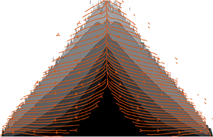
Figure 2. Force lines (solid grey) and random walk lines (dashed blue) in grain piles and silos. The dashed black line in each plot is the free surface. (a,b) Piles constructed by deposition from a funnel and by raining. (c,d) Silos with bumpy frictional walls and flat frictionless walls, respectively, both filled by raining.
For piles deposited from a funnel (figure 2a) and by raining (figure 2b), the force lines are vertical at the symmetry axis, but incline away from the vertical with increasing radial distance  $r$. The slope asymptotes to a constant at smaller $r$ for a funnel-deposited pile than for a rained pile. Thus, the difference between the two types of deposition is primarily in the core of the pile. The inclination of the force lines results in lateral outward transfer of the weight of the material, which explains the lowering of the stress around the apex of the pile. This results in a dip in the normal stress at the base below the apex for a funnel-deposited pile, reported in numerous studies (Jotaki & Moriyama Reference Jotaki and Moriyama1979; Smid & Novosad Reference Smid and Novosad1981; Vanel et al. Reference Vanel, Howell, Clark, Behringer and Clément1999; Geng et al. Reference Geng, Longhi, Behringer and Howell2001b; Zuriguel, Mullin & Rotter Reference Zuriguel, Mullin and Rotter2007; Ai et al. Reference Ai, Chen, Rotter and Ooi2011), and flattening of the stress profile below the apex for piles deposited by raining (Vanel et al. Reference Vanel, Howell, Clark, Behringer and Clément1999; Geng et al. Reference Geng, Longhi, Behringer and Howell2001b; Ai et al. Reference Ai, Chen, Rotter and Ooi2011). In silos, the nature of the walls has a strong influence on the orientation of the force lines. The results for bumpy frictional walls and smooth frictionless walls are shown in figure 2(c,d). For frictional walls, the force lines display a marked curvature towards the walls – thus the influence of the walls is felt deep inside the silo. When the walls are frictionless, the force lines incline slightly (figure 2d) from the vertical with distance from the symmetry axis. The slope of the force lines at the walls is indicative of traction on the walls: the more they deviate from the vertical, the greater is the traction.
What determines the orientation of the force lines? To answer this question, we consider the flow during the process of deposition, shown in the supplementary movies available at https://doi.org/10.1017/jfm.2024.6; representative snapshots of some of the movies are shown in figures 7 and 8 in Appendix B. Supplementary movies 1 and 2 show streamlines of the (volume and ensemble averaged) velocity field in piles. They reveal a strong horizontal outward component in the flow that spans the entire pile for deposition from a funnel, but is absent in the core for deposition by raining. The horizontal flow is contrary to the assumption of most previous studies that a pile is formed by flow and accretion along the sloping surface (Wittmer et al. Reference Wittmer, Claudin, Cates and Bouchaud1996; Vanel et al. Reference Vanel, Howell, Clark, Behringer and Clément1999; Rajchenbach Reference Rajchenbach2001; Atman et al. Reference Atman, Brunet, Geng, Reydellet, Claudin, Behringer and Clément2005). The background colour in the movies represents the magnitude of the displacement  $\boldsymbol {s}$ in a short time interval; its spatial variation shows that the material undergoes shear in the vertical direction. For simple shear, the probability of finding a contact below is maximum along the compression axis (i.e. at an angle of $\pi /4$ from the $z$ axis in the anti-clockwise direction, see figure 1). Though the flow in the pile is more complex, the horizontal flow and the ensuing shear results in asymmetry of contacts and contact forces about the vertical, which is frozen on cessation of flow (figure 2a,b). The evolution of the force lines, shown in supplementary movies 3 and 4, can now be understood: in a funnel-deposited pile, the outward orientation of the force lines starts from the early stages of pile formation, correlating well with the strong outward horizontal flow at all time. When deposition is by raining, the force lines are vertical in the core of the pile and begin to slope outwards in the regions of horizontal flow at the periphery of the growing pile. The flow in silos depends strongly on the nature of the side walls. For frictional walls, there is a clear outward flow towards the walls near the moving free surface (supplementary movie 5), leading to asymmetry in contacts and force transmission (supplementary movie 6). However, when the walls are smooth and frictionless, we see intermittent vertical creep along the entire height of the column (supplementary movie 7) for a substantial period after deposition. The time evolution of the flow and contact lines clearly suggest that the vertical creep determines the force network in the eventual static state (supplementary movie 8).
2.2. Load transmission through biased random walks
The insight gained from the force lines in figure 2 and the supplementary movies provides an understanding of the mechanism of stress transmission. Starting from any particle and moving downwards along contacts, the force paths are random walks if at each step, all contacts below have equal probability. The presence of a systematic contact and force asymmetry results in a biased random walk. This hypothesis can be readily tested using the simulation data: we assume that the weight of a particle is transmitted equally by all random walks starting from it, and incorporate the bias by weighting the probability of each step by the magnitude of the contact force. Thus, a random walk proceeds from particles  $i$ to $j$ below with transition probability $p_{ij}= |\boldsymbol {f}_{\!\!ij}|/\sum _k |\boldsymbol {f}_{\!\!ik}|$, where the sum is over contacts with particles $k$ below. The fraction of the weight $w_a$ of particle $a$ transmitted through the contact $ij$ is then the number of random walks $R_{ij}^a$ starting from $a$ and passing through $ij$ divided by the total number of random walks $R^a$ starting from $a$. The random walk estimate of the fraction of the total weight transmitted through contact $ij$ then is $F_{ij} = \sum _a R_{ij}^a w_a/R^a$, the sum being over all particles $a$ above the contact $ij$. From $F_{ij}$, we define a force-weighted unit vector for particle $i$ as $\boldsymbol {f}_i^{rw} = \sum _j \boldsymbol {n}_{ij} F_{ij}/\sum _j F_{ij}$, where $\boldsymbol {n}_{ij}$ is the unit normal at the $ij$ contact. We then determine the volume and ensemble averaged unit vector field $\boldsymbol {f}^{rw} (x)$ and construct its ‘streamlines’ in the same manner as the force lines in § 2.1 – we refer to them as random walk lines.
We see in figure 2(a–d) that the random walk lines are indistinguishable from the force lines. Another way to verify this correspondence is by determining the vertical traction on the boundaries from the random walk estimates of the particle-wall contact forces (using the relation for  $F_{ij}$ above, but with $j$ being a wall particle). Here again we see close agreement between the random walk estimate and the actual stress obtained from the DEM simulations in figure 4(a–c). We have thus established that the paths of force transmission are essentially ensemble averaged biased random walks.
2.3. Closure relation for the stress
We now show that in the continuum limit, the picture of force transmission by biased random walks leads to a closure relation for the stress. Consider particle  $i$ with coordinates ( $\boldsymbol {x}_{\perp i}, z_i$), where $\boldsymbol {x}_{\perp i}$ is the vector of coordinates along axes perpendicular to gravity. Load is transmitted to it via random walks from particles $j$ above that are in contact with $i$. Particle $j$ transmits load to its contacts below with transition probability $p_{jk}$ (such that $\sum _{k} p_{jk} =1$). The load on $i$ then is
 \begin{equation} {\mathcal{L}}(\boldsymbol{x}_{{\perp} i}, z_i) = \sum_{j} [{\mathcal{L}}(\boldsymbol{x}_{{\perp} j}, z_j ) + m_j g ] p_{ji} (\boldsymbol{x}_{{\perp} j}, z_j ), \end{equation}
where  $m_j$ is the mass of $j$ and $g$ the gravitational acceleration. We now average (2.1) over an ensemble of realisations and a small elemental volume $\Delta A_\perp \Delta z$ to obtain the smoothed form
 \begin{align} {\mathcal{L}}(\boldsymbol{x}_{{\perp}}, z) &= \int {\mathcal{L}}(\boldsymbol{x}_{{\perp}} - \Delta \boldsymbol{x}_{{\perp}}, z - \Delta z) p(\boldsymbol{x}_{{\perp}} - \Delta \boldsymbol{x}_{{\perp}}, z - \Delta z, \Delta \boldsymbol{x}_{{\perp}}, \Delta z)\, {\mathrm d} \Delta \boldsymbol{x}_{{\perp}}\nonumber\\ &\quad + \rho g \Delta A_\perp \Delta z, \end{align}
where  $p(\boldsymbol {x}_{\perp }, z,\Delta \boldsymbol {x}_{\perp }, \Delta z)$ is the transition probability for the load to be transmitted from $\boldsymbol {x}_{\perp }$ to $\boldsymbol {x}_{\perp }$ + $\Delta \boldsymbol {x}_{\perp }$ in the horizontal plane during a small vertical displacement $\Delta z$ (satisfying the normality constraint $\int p (\boldsymbol {x}_{\perp }, z, \Delta \boldsymbol {x}_{\perp }, \Delta z)\, {\mathrm d} \Delta \boldsymbol {x}_{\perp } = 1$), the integral being over all $\Delta \boldsymbol {x}_{\perp }$. Equation (2.2) is the Chapman–Kolmogorov equation for a Markov process (McQuarrie Reference McQuarrie1976, § 20-2), extended to include a source term (the body force); ${\mathcal {L}}$ and $p$ are now smoothly varying functions of $\boldsymbol {x}_{\perp }$ and $z$. Expanding the integrand in Taylor's series about ( $\boldsymbol {x}_{\perp }, z$) and retaining only terms up to $O(|\Delta \boldsymbol {x}_{\perp }|^2)$ and $O(\Delta z)$, we get
 \begin{equation} \bar{\mathcal{L}} = \int [ 1 - \Delta \boldsymbol{x}_{{\perp}} \boldsymbol{\cdot} \boldsymbol{\nabla} + \tfrac{1}{2} \Delta \boldsymbol{x}_{{\perp}} \Delta \boldsymbol{x}_{{\perp}} \boldsymbol{:} \boldsymbol{\nabla}_{\! \perp} \boldsymbol{\nabla}_{\! \perp} - \Delta z \partial z](\bar{\mathcal{L}} p)\, {\mathrm d} \Delta \boldsymbol{x}_{{\perp}} + \rho g \Delta z, \end{equation}
where  $\bar {\mathcal {L}} \equiv {\mathcal {L}}/\Delta A_\perp$ and $\boldsymbol {\nabla }_{\! \perp }$ is the gradient operator in $\boldsymbol {x}_{\perp }$. Rearranging (2.3), we get
 \begin{equation} \frac{\partial \bar{\mathcal{L}}}{\partial z} ={-} \boldsymbol{\nabla}_{\! \perp} \boldsymbol{\cdot} (\boldsymbol{u} \bar{\mathcal{L}}) + \boldsymbol{\nabla}_{\! \perp} \boldsymbol{\cdot} (\boldsymbol{\mathsf{D}} \boldsymbol{\cdot} \boldsymbol{\nabla}_{\! \perp} \bar{\mathcal{L}}) + \rho g. \end{equation}
Here  $\boldsymbol {u} = \langle \Delta \boldsymbol {x}_{\perp } \rangle /\Delta z$ is the drift velocity and $\boldsymbol{\mathsf{D}} = \langle \Delta \boldsymbol {x}_{\perp }' \Delta \boldsymbol {x}_{\perp }' \rangle /(2\Delta z)$ is the diffusivity tensor, where we have used the notation $\langle \xi \rangle \equiv \int \xi p \, {\mathrm d} \Delta \boldsymbol {x}_{\perp }$ for the mean of $\xi$ and $\xi ' \equiv \xi - \langle \xi \rangle$ for its deviation from the mean. Assuming $\boldsymbol{\mathsf{D}}$ to be isotropic (which we verify in the simulations), $\boldsymbol{\mathsf{D}} = D\,\boldsymbol {\delta }$, where $\boldsymbol {\delta }$ is the identity tensor. Equation (2.4) has the form of an unsteady advection-diffusion equation, with $z$ being the time-like variable. Recognising that $\bar {\mathcal {L}}$ is the vertical normal stress $\sigma _{zz}$ and comparing (2.4) with the $z$ component of the static momentum balance $\partial \sigma _{zz}/\partial z + \partial \sigma _{xz}/\partial x + \partial \sigma _{yz}/\partial y = \rho g$ in Cartesian coordinates ( $x, y, z$), we get
 \begin{equation} \sigma_{xz} = u_x \sigma_{zz} - \frac{\partial}{\partial x}(D \sigma_{zz}) ,\quad \sigma_{yz}= u_y \sigma_{zz} - \frac{\partial}{\partial y}(D \sigma_{zz}). \end{equation}
Equation (2.5a) is a full closure for the momentum balances in 2-D (i.e. in the  $x$–
$x$– $z$ plane). For 3-D problems, in addition to (2.5a,b), a closure is required to determine $\sigma _{xy}$. We propose $\sigma _{xy} = 0$, based on the expectation that shear stress on a vertical plane will only be in the direction of gravity, as the flow during deposition is expected to be along vertical planes; this will not be the case when there is a swirl flow during deposition. The PDE governing $\sigma _{zz}$ is parabolic, in contrast to plasticity and the FPA/OSL closures which yield hyperbolic PDEs, and elasticity-based closures which yield elliptic PDEs (see § 1). For 2-D problems, (2.5a) in the absence of diffusion is a linear algebraic relation between the shear and normal stresses. The FPA and OSL models (Wittmer et al. Reference Wittmer, Claudin, Cates and Bouchaud1996; Cates et al. Reference Cates, Wittmer, Bouchaud and Claudin1998) also proposed an algebraic closure relation of the form $\sigma _{xx} = \eta _1 \sigma _{zz} + \eta _2 \sigma _{xz}$, but it does not reduce to (2.5a) for any finite values of the constants $\eta _1$ and $\eta _2$. Moreover, one cannot discount diffusion in a disordered grain assembly. Most importantly, the drift velocity is not constant but spatially varying, implying that the orientations of the principal stresses must also be spatially varying, whereas the FPA and OSL models assume constant orientation. A convection-diffusion equation for $\sigma _{zz}$ was envisaged by Rajchenbach (Reference Rajchenbach2001) by extending the toy $q$ model to incorporate an assumed directional bias, but they did not identify the lateral dispersion of load as the shear stress. We have arrived at (2.5a,b) by showing that the paths of load transmission are ensemble averaged biased random walks in the contact network, thereby giving it a firm physical basis.
2.4. Application to piles and silos
We now apply (2.5a,b) to a conical pile and a rectangular silo; for the former, the momentum balances and the closure relation (2.5a,b) are posed in cylindrical coordinates ( $r, \theta, z$). The boundary conditions for the axisymmetric pile are the symmetry condition $\sigma _{rz} = 0$ at the axis, and zero normal and shear stress at the free surface. For the rectangular silo too, the symmetry condition $\sigma _{xz} = 0$ holds at $x=0$, but there is no obvious choice for the boundary condition at the walls. We impose the condition that the ratio of the contributions to $\sigma _{xz}$ from diffusion and advection is a constant $\alpha$,
 \begin{equation} \frac{-D \partial\sigma_{zz}/\partial x}{u_x \sigma_{zz}} = \alpha, \end{equation}
which is equivalent to the friction boundary condition  $\sigma _{xz}/\sigma _{zz} = K \mu _w$ used in the Janssen solution (Janssen Reference Janssen1895; Rao & Nott Reference Rao and Nott2008) if $\alpha = K \mu _w/u_x - 1$. The constant $\alpha$ must be $-1$ for frictionless walls ( $\sigma _{xz} = 0$); for bumpy frictional walls, it was taken to be 0 (i.e. the diffusive contribution to $\sigma _{xz}$ is negligible).
For each problem, the diffusivity and drift velocity were determined by conducting random walks in the respective force networks, the details of which are given in Appendix E. The diffusivity is found to be constant in all the cases at  $D = 1.41 d_p$. The spatial variations of the drift velocity for all the problems are shown in figure 3, and the fitted functional forms are
 \begin{equation} u_r = 0.28(r/R)^{0.29}, \quad u_r = 0.32 (r/R_z) + 0.3 (r/R_z)^2 - 0.44 (r/R_z)^3 \end{equation}
for the funnel-deposited and rained piles, respectively, and
 \begin{equation} u_x = 0.17 \sinh (0.135 x/d_p), \quad u_x = 1.3 \times 10^{{-}3} x/d_p \end{equation}
for silos with bumpy frictional walls and smooth frictionless walls, respectively. In (2.7b),  $R_z$ is the radius of the pile at depth $z$.
$z$.

Figure 3. Profiles of the drift velocity in (a) piles deposited by a funnel and by raining, and (b) silos with frictional and frictionless walls filled by raining. In funnel-deposited piles,  $u_r$ is largely independent of $z$, and hence $\hat {r} = r/R$. In piles deposited by raining, $u_r$ is a function of $r$ and $z$, but the profiles for different $z$ collapse to a single curve if $r$ is scaled by the radius of the pile $R_z$ at depth $z$, and hence $\hat {r} = r/R_z$. More details are given in Appendix E.
The stress field is obtained by solving the momentum balances with the closure (2.5a,b), using these fitted forms of the drift velocity and the above-mentioned boundary conditions. Figure 4(a–c) compare the model predictions with the data from DEM simulations – it is evident that there is very good agreement. As discussed in § 2.2, the close agreement between the random walk estimates of the vertical traction on the base of the pile and side walls of the silo ( $\sigma _{zz}$ and $\sigma _{xz}$, respectively) with the simulation data is another validation of the model.

Figure 4. (a,b) Profiles of the normal and shear stresses at the base of grain piles deposited (a) by a funnel and (b) by raining. (c) Shear stress  $\sigma _{xz}$ on a side wall in a rectangular silo with bumpy frictional walls and the normal stress $\sigma _{zz}$ (averaged over the cross-section) in a silo with smooth frictionless walls. In panels (a–c), the grey squares are data from DEM simulations, the blue circles are estimates from the biased random walks, and the black solid and dashed lines are the predictions of the advection-diffusion model. (d) Profiles of the drift velocity $u_x(x)$ for 2-D silos (see Appendix A) with bumpy frictional walls of different width $W$.
$W$.
To further demonstrate the validity of the model, we apply it to a silo filled by an unusual peripheral deposition method (figure 5a), wherein grains flow into a cylindrical silo from an annular inlet adjacent to the silo wall. The flow of grains from the periphery causes the force lines to slope towards the centre and an inward slope of the free surface (figure 5b). The slope of the force lines implies that the weight of the material is transferred inward towards the centre. This is indeed seen in figure 5(c), where  $\sigma _{zz}$ on the base is maximum at the centre, despite the height of the free surface there being minimum. The predicted stress profile at the base, using the fit
 \begin{equation} u_r ={-}0.1 + 6.6 \times 10^{{-}4}\exp(0.148 r/d_p) \end{equation}
for the drift velocity (see Appendix E), is in close agreement with the simulation data (figure 5c).

Figure 5. (a) Schematic of peripheral filling of a cylindrical silo. The granular material discharges into the silo as the inner cylinder is retracted upwards. (b) Force lines for the peripherally filled silo. The dashed line is the free surface. (c) Radial variation of the normal and shear stresses at the base.
A pertinent question is how the model may be used in a geometry for which the functional form of  $\boldsymbol {u}$ is unknown. An answer is suggested by figure 4(d), where it is seen that the profiles of $u_x$ in silos of a wide range of the silo width $W$ collapse to a single curve when each is scaled by the value $u_x^w$ at the walls (also see Appendix D). Thus, for a given silo width $W$,
$W$,  $u_x^w$ is the sole fitting parameter. Moreover, $D$ and $u_x$ can also be measured by experiments, as discussed in § 3.
Despite the potential difficulty in determining the drift velocity, we believe we have made a useful advance by identifying the correct mathematical form of the closure for the static stress. Moreover, the closure implies non-trivial aspects of the spatial variation of stress. This point is illustrated by considering two simple stress fields that satisfy momentum balance, but are incompatible with (2.5a,b).
Lithostatic stress. For a granular bed that is unbounded in the lateral direction, the lithostatic stress field is
 \begin{equation} \sigma_{zz} = \rho g z + h(x), \quad \sigma_{xz} = 0, \end{equation}
where  $h(x)$ is the normal traction on the boundary $z = 0$ due to a load placed on the bed. It signifies that the overburden at each point is transmitted vertically downwards. However, substituting (2.10a,b) in (2.5a) yields $u_x = D h'(x)/(z + h(x))$, which implies that the $\sigma _{zz}$ is transferred laterally from regions of low overburden to high overburden. Thus, (2.10a,b) is incompatible with (2.5a) unless $D$ vanishes identically; however, $D$ can only vanish for a perfectly ordered assembly. For a disordered grain assembly, diffusion of $\sigma _{zz}$ from regions of high to low overburden is an important feature of our model and an intuitively desirable one.
Stress in a silo. For a grain column enclosed by frictional vertical walls (figure 1b), the following stress field satisfies momentum balance and obeys the well-known Janssen saturation, mentioned in § 1:
 \begin{equation} \sigma_{zz} = \rho g \alpha^{{-}1} ( 1 - {\rm e}^{-\alpha z} ),\quad \sigma_{xz} = \rho g x ( 1 - {\rm e}^{-\alpha z} ), \end{equation}
where  $\alpha = K \mu _w/W$, $K$ is the ratio $\sigma _{xx}/\sigma _{zz}$ at the lateral walls ( $x= 0, W$) and $\mu _w$ is the wall friction coefficient. Substituting this stress field in (2.5a) yields $u_x = \alpha x$, implying that $\sigma _{zz}$ should increase along the curve ${{\rm d} x}/{\rm d}z = \alpha x$. This contradicts the assumed $\sigma _{zz}$ profile (2.11a), which varies only along $z$. Note that in this case, there is no lateral diffusion of $\sigma _{zz}$ as it is independent of $x$. Our model (2.5a,b) yields a stress field that obeys Janssen saturation, but its variation with $x$ is more complex.
The above examples convey the key non-trivial features of our closure: the first is that load is in general transmitted laterally due to advection and diffusion. The second feature is that when there is a lateral variation of  $\sigma _{zz}$, the shear stress $\sigma _{xz}$ is non-zero except in special circumstances where advection and diffusion exactly cancel each other.
3. Summary and discussion
This paper makes two main contributions. The first is the definition of the force lines in a static granular assembly under gravity, and the demonstration that they are an insightful representation of load transmission and encode deposition history. The second is the hypothesis that paths of load transmission are biased random walks, and its validation by showing that the ensemble averaged random walks coincide with the force lines. This recognition leads to an advection-diffusion equation for the vertical normal stress and, thereby, a closure relation for the static stress. Diffusion arises from disorder in the contact network and advection from the directional bias of the contact force due to shear generated by the horizontal flow during deposition. The closure relation is simple and applicable to all geometries and types of gravity deposition. Its predictions are in good agreement with data from DEM simulations for piles and silos constructed by different deposition methods.
An important aspect of our findings is that the drift velocity  $\boldsymbol {u}$ is spatially varying and sensitive to the deposition method and the nature of the boundaries. For the model to be of practical utility, methods must be found to determine $\boldsymbol {u}(\boldsymbol {x}_\perp,z)$. In this paper, we have obtained it from the force network derived from our DEM simulations as a proof of concept, but there are other ways of obtaining it. We envisage experimental methods to infer $\boldsymbol {u}$, such as through transmission of acoustic waves, used quite routinely to determine the properties of inhomogeneous and anisotropic materials, such as in seismic imaging (Wang Reference Wang2016). Moreover, we have shown that DEM simulations of a small but dimensionally similar system provide a good estimate of the spatial variation $\boldsymbol {u}$ (figure 4d). In ongoing work, we have preliminary results to show that the functional form of $u_x(\hat {x},z)$ for deposition by raining channels and hoppers is the same for all $z$, where $\hat {x} = x/W(z)$ and $W(z)$ is the container width at depth $z$. This gives us hope that an expression for $\boldsymbol {u}$ can be found that will have validity for a class of geometries, such as containers with convex walls. We therefore believe it is possible to classify geometries and deposition protocols and arrive at general relations for $\boldsymbol {u}$.
We now discuss the distinction (or relation) between our closure relation (2.5a,b) and those proposed in previous studies. As discussed in § 2.3, the physical arguments on which our closure rests are quite different from those of the FPA and OSL closures, and so too is the mathematical form of the equations governing the stress. Using our closure, the momentum balance in the gravity direction gets decoupled from the balances in the lateral directions. Moreover, the spatial variation of  $\boldsymbol {u}$ implies that the directions of the principal stresses are not constant. Coming to elastic and elastoplastic models, it is obvious that the contact forces on individual grains are elastoplastic – indeed, the contact force between grains at rest is elastoplastic in DEM. It therefore follows that the stress averaged over a mesoscale of a few grains must be elastoplastic. However, the fabric of the granular medium is anisotropic and spatially varying (as shown by figure 2), making the elastoplastic description much more complex at macroscopic scales. Our closure captures the anisotropic and spatially varying fabric in a simple manner; we therefore see it as a simple model with an appealing microscopic basis, but not a negation of elastoplastic descriptions. For example, the splay and curvature of the force lines in a silo capture the elastic-like spreading of the load.
As discussed in § 1, experimental studies have been largely restricted to simple geometries, small systems and rather artificial deposition protocols. It is desirable to have more experiments to test our closure for the static stress and also resolve the disparate findings of previous experimental studies. In particular, measurement of the stress in grain assemblies created by different deposition methods and in complex geometries would be useful. It would also be of value to use measurements of the contact forces using photoelastic disks (Geng et al. Reference Geng, Reydellet, Clement and Behringer2003) to more directly validate the utility of force lines.
Finally, we note that this is the first step in developing a closure for the stress in static granular media. The closure is limited to a fixed gravity direction and wall orientations. One could envisage more complex depositions where the wall orientations relative to the direction of gravity vary in time. If the variation is slow, we expect that at each instant, the form of the closure (2.5a,b) would still be valid, but  $\boldsymbol {u}$ and $D$ would be much more complex spatial functions. These are problems worth tackling due to their obvious practical importance, such as in industrial blenders.
Supplementary movies
Supplementary movies are available at https://doi.org/10.1017/jfm.2024.6.
Acknowledgements
We acknowledge the useful suggestions of an anonymous reviewer.
Funding
This work was supported by the Science and Engineering Research Board under grant EMR/2016/002817 and the International Fine Particle Research Institute.
Declaration of interests
The authors report no conflict of interest.
Appendix A. Method of deposition
To simulate the deposition of particles from a narrow source (funnel) and raining from a distributed source (sieve), we used the following protocol. A deposition region (shaded grey in figure 6a–c) of suitable size was chosen within which non-overlapping particles were randomly created to a volume fraction of 0.1 for narrow source deposition and 0.01 for raining, and allowed to fall under gravity. As particles drained from the deposition region, new particles were created and the process repeated until the required number of particles were deposited. The simulations were further continued until the kinetic energy per particle decreased to below  $10^{-10}m_p g d_p$, where $m_p$ is the mass of a particle of diameter $d_p$. For the 3-D piles and silos discussed in figures 2 and 3 of the paper, the deposition region had the shape of a cylinder and cuboid, respectively. For the 2-D simulations conducted to make the supplementary movies, obtain the data for figure 3(d), and determine the diffusivity $D$ (see Appendix E), the deposition zone was a thin cuboid that held a monolayer of particles of area fraction 0.2. The particles were constrained to remain in the plane after leaving the deposition region, thereby forming 2-D piles and silos.

Figure 6. Schematic of the deposition procedures used for creating piles and filling silos. (a,b) Creating a pile from a narrow source and by raining. (c) Filling a rectangular silo by raining. (d) Peripheral deposition of a cylindrical silo: the figures from left to right show the initial, intermediate and final states of deposition.
A.1. Pile
For funnel-deposited conical piles, the deposition region was a cylinder of length  $L_{d} = 60d_p$ and radius $R_{d} = W_{d}/2 = 7d_p$ (see figure 6a). For 2-D piles, the deposition region was a thin cuboid that held a monolayer of particles with dimensions $L_{d} = 50d_p$, $W_{d} = 10d_p$. The lower boundary of the deposition region was at a height $H_{d} = 50d_p$ from the base.
For conical piles deposited by raining, the deposition region was a cylinder of length  $L_{d} = 10d_p$ and radius $R_{d} = W_{d}/2 = R$ (figure 6b). The lower boundary of the deposition region was at a height $H_{d} = 90d_p$ from the base. For 2-D piles, the corresponding dimensions of the deposition region were $L_{d} = 50d_p$, $W_{d} = 2R$ and $H_{d} = 60d_p$.
In both deposition methods, particles at radial positions  $r > R$ exited the simulation cell, thereby forming a pile of radius $R$. This is equivalent to particles being poured on an elevated circular disk of radius $R$ in a physical experiment.
A.2. Rectangular silo
The 3-D silos were of rectangular cross-section with periodic boundaries in the  $y$ direction that were a distance $P = 25d_p$ apart. The cuboidal deposition region was of dimensions $L_{d} = 100d_p$, $W_{d} = 17d_p$, and periodic in the $y$ direction with depth $P$. Its lower boundary was at a height $H_{d} = 300d_p$ from the base (figure 6c). For the 2-D silos, the corresponding dimensions of the deposition region were $W_{d} = W - 3 d_p$ and $H_{d}\approx H + 10d_p$.
A.3. Cylindrical silo filled by peripheral deposition
The required number of particles were first rained into an annular region bounded by the inner and outer cylinders of radii  $R_i =30d_p$ and $R = 40d_p$ (figure 6d). After reaching a static state, the inner cylinder was lifted with constant speed $v_w = 0.8\sqrt {gd_p}$, resulting in the flow of particles from the periphery towards the centre. The simulations were continued until all particles exited the annular region and the kinetic energy per particle fell to below $10^{-10}m_p g d_p$. At the static state, the conical free surface sloped inwards at an angle $23^\circ$ from the horizontal and the height at the periphery is $H = 52d_p$.
Appendix B. Snapshots of the flow streamlines and the force lines
As discussed in § 2.1, supplementary movies 1–4 show the streamlines of the velocity field and the evolution of the force lines during deposition of the pile, and movies 5–8 show the same for filling of a silo. To aid the reader, snapshots of the streamlines and the force lines are shown in figure 7 for the funnel-deposited pile and in figure 8 for the silo with bumpy frictional walls (filled by raining). The snapshots convey the relation between the lateral outward flow and the orientation of the flow lines, which is much clearer in the movies.

Figure 7. Snapshots of (a–c) the streamlines and (d–f) the force lines (taken from supplementary movies 1 and 3, respectively) during deposition of a 2-D pile from a funnel. The snapshots are at times (a,d) 162, (b,e) 649 and (c,f) 1137 in units of  $(d_p/g)^{1/2}$ from the start of filling. The background colour in panels (a–c) represents the magnitude of the displacement $\boldsymbol {s}$ in a time interval $8.12(d_p/g)^{1/2}$. The background colour in panels (d–f) is the scaled deposition time $\lambda \equiv t/T$, where $t$ is the time at which the material leaves the deposition region and $T$ the time at which the deposition region is emptied.

Figure 8. Snapshots of (a–c) the streamlines and (d–f) the force lines (taken from supplementary movies 5 and 6, respectively) during filling of a silo with bumpy frictional walls. The snapshots are at times (a,d) 81, (b,e) 243 and (c,f) 406 in units of  $(d_p/g)^{1/2}$ from the start of deposition. The $z$ axis in panels (a–c) is shifted with time to clearly show the flow in the growing free surface region. The meaning of the background colour is the same as in figure 7.
Appendix C. Force lines determined from the total contact force
The force lines in figure 2 were computed from the normal contact force  $\boldsymbol {f}^{{n}}_{ij} = \boldsymbol {n}_{ij} \boldsymbol {{\cdot }} \boldsymbol {f}_{ij} \boldsymbol {n}_{ij}$ between any two particles $i$ and $j$ in contact, where $\boldsymbol {n}_{ij}$ is the unit normal at the point of contact. However, they could just as easily be determined from the total contact force $\boldsymbol {f}_{ij}$, and the results are shown in figure 9. It is evident that the force lines determined from the total and normal contact forces are nearly identical.

Figure 9. Comparison of the force lines determined from the total contact force (dashed red) with the force lines determined from the normal contact force (solid grey). (a,b) 2-D piles constructed by deposition from a funnel and by raining. (c) 3-D rectangular silo with bumpy frictional walls filled by raining.
Appendix D. The effect of system size on the force lines
To understand the influence of the system size on the spatial variation of the force lines, we studied 2-D silos with rough frictional walls for a range of the silo width  $W$. Keeping the aspect ratio $H/W$ roughly constant (between 10 and 12), we studied silos of widths $W=20$, 40, 90, 140 and $200d_p$. Figure 10 shows that the features of the force lines for silos of width $W= 20d_p$ and $W = 140d_p$ are very similar. To make a quantitative comparison, we determined the horizontal variation of the advection velocity $u_x$ (see Appendix E) at a depth $z = 7W$ from the free surface for a range of $W$. Figure 4(d) shows that the $u_x(x)$ profiles, when scaled by the value $u_x^w$ at the wall, collapse to a single curve. This suggests that the influence of the walls is felt deep inside the silo, no matter how large the width is.

Figure 10. Force lines (solid grey) and random walk lines (dashed blue) in 2-D silos of two widths (a)  $W=20d_p$ and (b) $W=140d_p$.
A related point is the influence of the deposition height  $H_d$ (see figure 6) on the force lines. We studied the force lines for deposition heights $H_d = 45d_p$ and $60d_p$ for funnel deposited 2-D piles and found that the orientation of the force lines for the different $H_d$ differ only near the free surface. They are independent of $H_d$ deeper in the pile, plausibly because particles lose their kinetic energy within a short distance of their entry to the pile, whence the flow inside the pile during deposition is non-inertial.
Appendix E. Determination of the drift velocity and diffusivity
As advection is unidirectional for the rectangular silo, the drift velocity  $u_x = \lim _{\Delta z \to 0} \langle \Delta x \rangle /\Delta z$ at any point is simply the slope of the random walk line (and therefore the force line) passing through that point; the same holds for $u_r$ in the axisymmetric pile.
Figure 11(a) shows the variation of the drift velocity  $u_x$ with $x$ in the silo with bumpy frictional walls (corresponding to figure 2c) at five different depths $z$, where it is evident that $u_x$ is nearly independent of $z$. The functional form for $u_x(x)$ is therefore obtained by averaging over the range of depth $0.2H < z < H$, shown in figure 11(b), and the fitted form is given in (2.8a). The same conclusion is reached for the silo with frictionless walls (corresponding to figure 2d), though the data are noisier due to the small magnitude of $u_x$ (figure 11c); the fitted form obtained from the data in figure 11(d) is given in (2.8b).

Figure 11. (a) Drift velocity  $u_x$ in a rectangular silo with bumpy frictional walls at five different depths. (b) Average of $u_x$ in panel (a) over the range of depth $2H < z < H$, and the fitted curve for $u_x(x)$ whose algebraic form is given in (2.8a). (c) Drift velocity $u_x$ in a rectangular silo with smooth frictionless walls at different depths. (d) Average of $u_x$ in panel (c) over the range of depth $2H < z < H$ and the fitted curve for $u_x(x)$, whose algebraic form is given in (2.8b).
For funnel-deposited conical piles, we again find that  $u_r$ is largely independent of $z$ (figure 12a), except within a thin layer close to the sloping free surface which we ignore. The functional form for $u_r(r)$ is therefore obtained by averaging over the range of depth $0.2H < z < H$, and the fitted relation is given in (2.7a). For conical piles deposited by raining, $u_r$ is a function of $r$ and $z$ (figure 12c). However, a reasonable collapse of the profiles for all $z$ is obtained if $r$ is scaled by $R_z$, the radius of the pile at $z$, as shown in figure 12(d). The fitted relation for $u_r(r/R_z)$ is determined by averaging over the range of depth $0.2H < z < H$, which is given in (2.7b).

Figure 12. (a) Radial variation of the drift velocity  $u_r$ for a funnel deposited conical pile at three depths. (b) Average of $u_r$ over the range of depth $0.2H < z < H$ and the fitted curve for $u_r(r/R)$, whose algebraic form is given in (2.7a). (c) Radial variation of $u_r$ for a rained conical pile at three depths. (d) Collapse of the profiles of $u_r$ when $r$ is scaled by $R_z$, the pile radius at depth $z$. (e) Average of $u_r(r/R_z)$ over the range of depth $0.2H < z < H$ and the fitted curve, whose algebraic form is given in (2.7b).
Finally, for the cylindrical silo filled by peripheral deposition (figure 4), we again find that  $u_r$ is largely independent of $z$ (figure 13a). The functional form for $u_r(r)$ is therefore obtained by averaging over the range of depth $0.2H < z < H$ (figure 13b), and the fitted relation is given in (2.9).

Figure 13. (a) Radial variation of the drift velocity  $u_r$ for a cylindrical silo filled by peripheral deposition. (b) Average of $u_r$ over the range of depth $0.2H < z < H$ and the fitted curve for $u_r(r/R)$, whose algebraic form is given in (2.9).
The diffusivity is obtained by conducting random walks in the contact network. As mentioned in § 2.4, we find the diffusivity  $D$ to be nearly constant and the same for all geometries and deposition methods. To determine $D$, the variance $\langle |\Delta \boldsymbol {x}'|^2\rangle$ must be averaged over many random walks in the contact network. Since the drift velocity is spatially varying, every random walk experiences a different systematic lateral displacement. As a result, we find that the variance varies linearly with $\Delta z$ only for large values of the latter, and hence the system size must be large enough for accurate estimation of $D$. We therefore determined it from the largest system studied, namely a 2-D silo with rough frictional walls with $W= 140 d_p$ and $H = 1425 d_p$. We determined $\langle (\Delta x')^2\rangle$ from $10^4$ random walks starting from particles near the top of the silo and then averaging over all the realisations. As shown in figure 14, it is linear in $\Delta z$ only for $\Delta z > 150d_p$. The slope of the fitted line yields the estimate $D \equiv \langle (\Delta x')^2\rangle /(2\Delta z) = 1.41 d_p$.

Figure 14. Variance of the lateral displacement  $\langle (\Delta x')^2\rangle$ with the vertical displacement $\Delta z$. The red line is the fit for large $\Delta z$.


 Open access