


1. Introduction
Owing to their huge ice mass, large ice sheets exert considerable pressure on the underlying bedrock, which will respond with vertical movements to restore the equilibrium of forces. In the case of isostatic equilibrium, the resulting Earth depression is about one-third of the ice thickness, which can lead to the bedrock sinking in excess of 1 km under the thickest parts. It is generally believed that the interaction between the ice load and the underlying bedrock plays an important role in the dynamics and stability of these large ice sheets.
Broadly speaking, one can distinguish two major effects. First, there is the effect of bedrock adjustments on the ice-sheet surface elevation. A lowering of the surface will generally result in more melting and a lower mass balance, in turn lowering the surface even more. This creates a positive feed-back. In particular, the time delay of the isostatic adjustment process is often invoked as an important element in explaining the terminations of the Quaternary glacial cycles on the continents of the Northern Hemisphere (e.g. Oerlemans, 1981).
A second important aspect of ice Earth interactions is evident from the dynamics of the Antarctic ice sheet. Much of this ice sheet is presently surrounded by ice shelves, which interact with the grounded ice sheet and the environmental forcing in a complicated way, resulting in movements of the grounding line. Model studies on the large-scale behaviour of the Antarctic ice sheet during the Quaternary glacial cycles have pointed out that the most important environmental control on grounding-line migration is provided by eustatic sea-level changes (Huybrechts, 1990a, b). A lowering of the global sea-level stand, for instance, will cause an immediate advance of the grounding line in those areas where the free water depth is no longer able to float an ice shelf. Clearly, vertical isostatic displacements have a similar effect on the free water depth and thus provide an additional control on grounding-line migration. Here, also, the time response is crucial. The speed at which the bedrock rebounds during the retreat strongly influences the minimum size the West Antarctic ice sheet is likely to attain (Huybrechts, 1992).
Additionally, because of this time lag, the present bedrock is unlikely to have adjusted completely to its past loading history. One implication is that ongoing viscous uplift of the bedrock may result in a future advance of the grounding line in the Ross Sea area by several hundreds of kilometres (Greishar and Bentley, 1980). Such incomplete rebound is in line with a clear trend for negative isostatic gravity values in this area (Bentley and others, 1982) and this is also supported by modelling studies (Lingle and Clark, 1985).
From this overview, it is clear that the bedrock treatment in glacial-cycle simulations, both with respect to temporal and spatial patterns, will be crucial to the model outcome. Present-day large-scale ice-sheet models usually do not deal with the entire visco-elastic problem and usually revert to simple models for the lithospheric deflection and the ensuing viscous response of the underlying asthenosphere.
The aim of this paper is to compare the isostatic models commonly used in ice-sheet modelling with results obtained using a more sophisticated self-gravitating visco-elastic spherical Earth model. Only a few of these spherical models exist today (Peltier, 1974; Cathles, 1975; Lambeck and others, 1990; Spada and others, 1992; Le Meur, 1996) and, up to now, none of them has been fully coupled in an interactive way with a three-dimensional ice-sheet model. Such a bedrock model is devoid of many of the simplifying assumptions typical of the more usual methods and therefore it is thought to be more realistic. A comparison of these methods will be demonstrated by coupling the different bedrock treatments with a three-dimensional thermomechanical Antarctic ice sheet model applied to the last glacial cycle under the same forcing conditions.
Section 2 gives a short overview of the various methods tested. The results of intercomparison are presented in section 4, which is followed by a discussion on the most important drawbacks and advantages of each of these individual treatments of isostasy.
2. Treatment of Isostasy in Glaciological Models
The various methods used in present-day ice-sheet models dealing with isostasy all make a distinction between the behaviour of the lithosphere, which controls the geometric shape of the deformation, and the response of the underlying asthenosphere, which governs the time-dependent characteristics of the bedrock adjustment. Indeed, the planet can, in the first instance, be approximated by a thin elastic outer shell floating on a highly viscous asthenosphere according to Archimedes principle.
These methods can be classified according to the way the two Earth layers are treated. For the lithosphere there are two treatments. One neglects its flexural rigidity, making the response local (the model is then referred to as LL for local lithosphere). The other accounts for it, giving rise to a characteristic elastic deformation profile (referred to as EL for elastic lithosphere), which substantially deviates from the local one. As regards the asthenosphere, the two treatments approximate the time-lagged flow within the mantle either by using a diffusion equation (DA for diffusive asthenosphere) or by a purely exponentially decaying hydrostatic response function (RA for relaxed asthenosphere).
2.1. Treatment of the lithosphere
In the case of neglected flexural rigidity, the lithosphere only locally transmits the effects of the load to the asthenosphere. Geometrically speaking, there is, in fact, no lithospheric effect at all, since the result would be exactly the same as if the ice were floating directly on the asthenosphere, like an iceberg on the sea. Therefore, given ice thickness H i, it becomes very easy to calculate the bedrock equilibrium depression h (positive downwards) according to
where ρi is the ice density (910 kg m−3) and ρa is the asthenosphere density (3300 kg m−3). Conversely, when the flexural rigidity is taken into account, one is now dealing with the bending of an elastic plate (Lliboutry, 1965; Brotchie and Silvester, 1969). In that case, one does not only consider the load just above, but one also integrates the contributions from more remote locations, which gives rise to deviations from local isostasy. The downward deflection w created by a point load q for a floating elastic plate is a solution of
where D represents the flexural rigidity (1 × 1025 Nm) and ρ a gw is the upward buoyancy force exerted on the deflected pan of the lithosphere inside the asthenosphere. The deflection at a normalized distance x = r/Lr from the point load can be written as
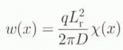
with χ(x) a Kelvin function of zero order, r the real distance from the load q and (L
r the so-called radius of relative stiffness  . A point load will cause a depression within a distance of four times L
r (L
r = 130 km for a 115 km thick lithosphere) and, beyond this distance, a small bulge appears. As lithosphere deflection is a linear process, the total deflection at each point is calculated as the sum of the contributions of all the neighbouring points within a distance of about five-six times L
r (650–780 km). The difference between the two methods LL and EL is most pronounced in the vicinity of the ire-sheet margin (Oerlemans and Van der Veen, 1984).
. A point load will cause a depression within a distance of four times L
r (L
r = 130 km for a 115 km thick lithosphere) and, beyond this distance, a small bulge appears. As lithosphere deflection is a linear process, the total deflection at each point is calculated as the sum of the contributions of all the neighbouring points within a distance of about five-six times L
r (650–780 km). The difference between the two methods LL and EL is most pronounced in the vicinity of the ire-sheet margin (Oerlemans and Van der Veen, 1984).
2.2. Treatment of the asthenosphere
The first way of accounting for the time-dependence of the isostatic response is simply to estimate the characteristic time constant τ, and to state that the speed of adjustment is proportional to the difference between the equilibrium profile w and the current profile h, and is inversely proportional to that time constant, leading to
in which w is the lithosphere deflection by either of the two methods described above, h is positive downwards and τ is taken as 3000 years in the experiments described in this paper. The coupling of Equation (1) with Equation (4) yields the LLRA model (local lithosphere, relaxed asthenosphere), which despite its simplicity has proven able to reproduce the major effects of the isostatic Earth response on the Long-term behaviour of the Northern Hemisphere ice sheets. Oerlemans (1980) found that a value of 10 000 years for τ gave the best fit to reproduce the 100 ka periodicity in the growth and decay cycle characteristic for these ice sheets. However, because of the relative simplicity of both his ice and Earth models, the ice-volume curve could not be reproduced in detail and it was admitted that not too much importance should be attributed to the value for τ.
The second way of treating the viscous time-dependent behaviour is to consider the equation of motion within the asthenosphere, where the flow is supposed to be inversely proportional to the dynamic viscosity v of the medium (Oerlemans and Van der Veen, 1984). The driving force comes from the lateral pressure gradient, with the pressure being proportional to w – h, the deviation with respect to the equilibrium profile. Thus, the horizontal velocity u as a function of depth z can be expressed as
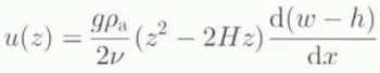
where H is the (rather artificial) depth below which no more influence is felt from above and ρa the asthenospheric density. Then, by expressing the principle of mass conservation, it is possible to relate the rate of bedrock sinking to the outflow of asthenospheric substratum under the form of a diffusion equation
No real attempt has been made to determine values for H and v, and the diffusion coefficient D a is usually inferred from rebound measurements over North America or Fennoscandia. The values usually adopted for D a range between 30 and 50 km2 a−1 (Oerlemans and Van der Veen, 1984; Huybrechts, 1992) and the experiments conducted here use the higher value of 50 km2 a−1. An often cited value for H is several hundred kilometres, which would, according to Equation (6), correspond to an upper mantle viscosity between 1 × 10¹⁹ and 1 × 10²⁰ Pa s. Again, depending on the expression for w, the two methods investigated in this paper are either LLDA (local lithosphere, diffusive asthenosphere), which is one of the commonest models used among ice-sheet modellers (e.g. Letréguilly and Ritz, 1993) or ELDA (elastic lithosphere, diffusive asthenosphere) as in Huybrechts (1992).
2.3. The full bedrock model SGVE
The self-gravitating visco-elaslic spherical Earth model (SGVE) was developed by Le Meur (1996) on the basis of Peltier’s previous work (Peltier, 1974, 1982, 1991b; Wu and Peltier. 1982). In this bedrock model, the entire Earth is considered, including an inviscid core, a lower and upper visco-elastic mantle and an elastic lithosphere. The asthenosphere (the actual asthenosphere plus the lower mantle), where most of the deformation takes place, is approximated by a Maxwell solid allowing for a full visco-elastic treatment according to the correspondence principle (Peltier, 1974). The derivation is made for a spherical Earth, not for a half-space as by Birchfield and Grumbine (1985). A decomposition into spherical harmonics associated with a space-unit load becomes particularly suitable. This assists in accounting for the complexity in the interactions between the spatial-displacement pattern and the gravity-field perturbation.
As the model is forced by a space unit-impulse load, the corresponding outputs, called the Green functions, only depend on the Earth parameters such as the density and the Lame parameter profiles (Dziewonski and Anderson, 1981), the mantle viscosity and the lithospheric thickness. The latter two parameters are the major unknowns and their correct determination has always been the subject of much debate. One way of inferring their values is to optimize a best fit between rebound data and isostatic models. In the present reference run, we used a lithosphere of 100 km thickness and a two-level mantle with a viscosity of 1 × 10²¹ Pa s for the lower part (below 670 km) and 5 × 10²⁰ Pa s for the upper part (670–100 km). These values are of the same order as those usually found in the literature (e.g. Mitrovica and Peltier; 1993, Fjeldskaar, 1994) and were chosen here on the ability of the model to yield an average characteristic response time of about 3000 years, which makes the comparison with the RA models relevant. One can notice that these two viscosities are somewhat different from the “best set” (1.5 × 10²¹ to 7.5 × 10²⁰) deduced from testing the same model over Fennoscandia (carried out later than the present study; Le Meur, 1996). However, they still yield realistic results with respect to matching the present-day rate of uplift over Fennoscandia and, to a lesser extent, the remaining displacements to come in the future (run 6 in this study from Le Meur).
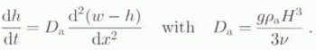
The isostatic response Y(x i , y j t) at the grid node (i,j) to a specified space-time loading scenario L s(x, y, t), where x and y are the two surface geographical variables and t is time, is obtained from the convolution of the appropriate Green function G(¸, t) with L s over the required time of memorization T m and space domain (a 1520 km square), leading to
where △x = △y is the 40 km spatial resolution, △i = △j is therefore set to 38 in order to sweep the required 1520 km square, and θ i 1, j 1 – θ ij represents the angular distance (in terms of co-latitude) between grid points (i 1, j 1) where L s is considered and the point where the summation is carried out (i, j).
In practice, the coupling with the ice-flow model is effectuated by feeding the isostatic model at 500 year intervals with a window that contains the ice-loading history L s over the preceding 30 000 years (T m). The latter period illustrates the ““memory effect”, which means that all the loading events that occurred during these past 30 000 years significantly contribute to the final deformation at time t. The new bedrock profile obtained every 500 years is then re-introduced into the glaciological model in an interactive way, which therefore is able to account fully for the influence of the Earth response on the ice dynamics.
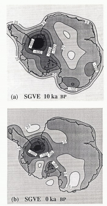
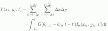
Fig. 1. Deviation from initial steady state for the reference model SGVE. (a) represents the difference in metres between the − ka BP bedrock elevation pattern and that from the reference run, whereas (b) is the same difference but for the present-day state. The expected bedrock rise below the Ronne-Filchner and Ross Ice Shelves is larger than the observed free-water depth in many places, indicating that a substantial part of these ice shelves would be replaced by grounded ice within a few thousand years.
The spectral method used here integrates ail harmonics up to degree 150, assuming that all spatial variations of the ice thickness occurring over wavelengths shorter than 266 km can be neglected. The validity of such an assumption essentially comes from the elastic behaviour of the lithosphere which acts as a “low-pass” filter and does not significantly bend under such short wavelength loads. In practice, this is easily observable with the rapid convergence of the results as the number of integrated harmonics increases. Finally, in order to match the 40 km grid spacing of the ice-sheet model, the Green function is calculated every 0.36 co-latitude degree with the corresponding Legendre polynomial.
3. Application to Modelling the Antarctic ICE Sheet
The five bedrock models described above were all coupled with a three-dimensional thermomechanical model for the entire Antarctic ice sheet applied to the last glacial cycle. The glaciological model includes an ice shelf, grounding-line dynamics and freely generates the ice-sheet geometry in response to a prescribed distribution of accumulation rate and surface temperature, as well as the global sea-level stand. Flow and temperature calculations are made on a three-dimensional grid with a horizontal resolution of 40 km and 11 layers in the vertical. The model has been documented in detail in Huybrechts (1992) with a description of a previous experiment on the last glacial cycle using an ELDA type of bedrock adjustment in Huybrechts (1990a).
The calculations started during the Eemian inter-glacial 126 000 years ago. Two forcing functions were used to drive the model. The Vostok temperature signal (Jouzel and others, 1993) was chosen to force the 10 m temperature and accumulation fields, and is assumed to be independent of latitude. Eustatic sea-level changes were derived from the Specmap record (Imbrie and others, 1984). In all these runs, an “interglacial reference run” was taken as the initial condition at 126 ka BP. This steady-state run was obtained by starting from the presently observed ice-sheet geometry (taken from the Scott Polar Research Institute (SPRI) maps; Drewry, 1983) and integrating the model under present-day climatic conditions until a stationary state was established. In obtaining this reference run, it was assumed that the observed present-day bedrock was in isostatic equilibrium with the observed present-day ice and water loading. Actually, as will be demonstrated further below, this may not be quite true but an alternative is not readily available.
4. Results of the Simulations
All five models are compared on the basis of the time-dependent evolution for the total ice volume and the mean bedrock elevation, and on the basis of the spatial patients for the present-day speed of uplift. We will treat the results from the SGVE model as a reference, as this approach is the most complete one.
4.1. Results from the SGVE model
Figure 1 displays the bedrock subsidence at two time intervals relative to the interglacial steady slate, which also served as an initial condition. The pattern for 1O ka BP (Fig. 1a) shows how far the bedrock has been depressed in response to the ongoing glaciation over Antarctica at a time about 2000 years before its glacial maximum. Not surprisingly, most of the depression takes place in West Antarctica, because that is where the hulk of the ice thickness changes are located, in particular, below and slightly inland of the two large present-day ice shelves (Huybrechts, 1992).

Fig. 2. Simulation of the total ice volume (a) and the mean bedrock elevation (b) for the Antarctic ice sheet during the last glacial cycle with the free bedrock parameterizations tested. The mean bedrock elevation is taken here over the entire Antarctic continent for bed elevations of h > −1500 m. An interesting feature to point out in the upper panel is that the deglaciation speed is nearly the same for each of the models.
The deviation from steady state at present (Fig. 1b] indicates how far the current bedrock surface is still out of isostatic equilibrium for the present climatic conditions. It is, in fact, a map of the remaining displacements to be expected in the future solely as a response to past changes in the loading history. It shows that the residual uplift is still up to 300 m in the Ronne Filchner basin and up to 100 m in the Ross Sea area, which reflects the different deglaciation histories of both ice shelves as simulated by the ice-sheet model (Huybrechts, 1990a).
The geographical patterns in Figure 1 also demonstrate several of the geometrical features characteristic of the Earth’s isostatic response. The most important feature occurs as a result of the bending of an elastic plate and finds its expression in the lateral effect of the loading away from the ice sheet into the ocean. Another point worth mentioning is the uplifted ocean floor in the plot for 10 ka BP, which is because of the lower sea level and hence the smaller water loading. The positive areas in figure 1b, illustrated by the + 25 m isoline a few hundred kilometres off the Antarctic coast, are more difficult to explain. They are probably the result of a complex interplay between the regional rise of the elastic litho-sphere, the collapse of a fore bulge and the subsidence of the ocean floor when the ocean fills again as a consequence of the deglaciation.
Figure 2 shows that the bedrock response is roughly in phase during the slow glacial build-up but that it clearly lags behind during the subsequent rapid deglaciation. Closer inspection of Figure 2 also reveals that it takes about 20 000 years for the global ice volume to recover a steady state after the environmental forcing reached present-day levels about 5000 years ago. This is not only due to the characteristic time-scale for the SGVE model (about 3000 years) but also because of the non-linearity produced by interaction with the ice sheet.
4.2. Comparison of the different methods
A first observation is that the total ice volume and mean bedrock elevation (Fig. 2) of all five methods roughly yield the same large-scale time-dependent behaviour. All ice-volume curves go up to a maximum at about 8000 years BP and then decrease to the present ice volume in a nearly synchronous way. The main difference between these methods is between the two diffusive models (ELDA and LLDA) and the three other models. The former exhibit a larger time lag and a smaller amplitude of the mean bedrock elevation. Both characteristics are inherent to the method and are explained further below.
In comparing patterns (Fig. 3), the present-day rate of uplift is worth examining for several reasons. First, the overall deglaciation speed is nearly the same from 5 ka BP up to the present for all five simulations (five almost parallel lines in figure 2a), indicating that each of the bedrock models has undergone a similar loading history for that period. Secondly, by dealing with speeds, one does not have to refer to any initial elevation pattern that can be different front one model to the other (e.g. the different minimal mean bedrock elevations at the glacial maximum; Fig. 2b).
The first major feature in Figure 3 is the different pattern of uplift for the two local lithosphere models compared to all the others. With a non-elastic lithosphere (LL), the response is not smoothed and is actually a local imprint of past ice-thickness changes. As there is no lateral effect beyond the load, as with an elastic lithosphere, the compensation of the ice-thickness variation is local and therefore also stronger. That is obvious from comparing ILRA with ELRA, which differ only by their lithospheric treatment. The highest uplift occurs in LLRA, with a maximum of 15 cm a−1 compared to less than 10 cm a−1 for ELRA.
The second clearly distinguishable feature is the concentric pattern obtained with the two diffusive models (DA), in which the central area of rebound is surrounded by a pronounced ring of lowering bed elevations. This is a direct consequence of the nature of the diffusion process, which implies that every vertical displacement of matter in the asthenosphere is compensated by an opposite movement in the near neighbourhood (“bulge effect”). When averaged over the entire surface of investigation to yield the mean bedrock elevation, the amplitude thus becomes less than with the other models, in spite of the higher local extreme values (−3.75–16.13 cm a−1 for ELDA and −22.91–40.19 cm a−1 for LLDA). It should be noted that LLDA overestimates the phenomenon (the “anti-bulge effect” in the present case of uplift), giving rise to abnormally strong negative speeds.
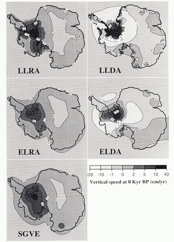
Fig. 3. Simulation of the present-day rate of uplift in cm a−1 over Antarctica for the five bedrock parameterizations. Acronyms are: LL, local lithosphere; EL, elastic lithosphere; RA, relaxed asthenosphere; DA, diffusive asthenosphere. The best agreement with SGVE, the self-gravitating visco-elastic model comes from ELRA with a very similar pattern and very close extreme values.
Finally, from the four parameterizations, it is clear that ELRA corresponds best to the reference simulation regarding both the geographical distribution and the extreme values for the uplift (−0.22–9.79 cm a−1 for ELRA and −0.25–10.91 cm a−1 for SGVE).
5. Discussion
On the basis of the results presented above, it becomes possible to point out the main advantages and drawbacks of these methods and to determine which ones are most appropriate.
First of all, a local lithospheric response (LL) cannot be considered as very realistic. This not only follows from the results presented here, but it is also supported by the geological evidence (e.g. plate tectonics) and by recent modelling, which finds it necessary to include the flexure of the lithosphere to reproduce correctly the main isostatic features (Lambeck and others, 1990; Fjeldskaar and Cathles, 1991; Le Meur, 1996). Therefore, the EL lithospheric treatment provides a significant improvement to reproduce better the geographical pattern. Summing a relation like Equation (3) has also become a relatively easy task with present-day computers. However, the results are rather sensitive to the value for the flexural rigidity D, so that a correct choice of this parameter is essential to determine the bending behaviour and the regional character of the plate deformation. For instance, there are indications that the lithospheric thickness is not uniform over Antarctica and is a factor of 5 less in West Antarctica (Stern and ten Brink, 1989). This corresponds to a flexural rigidity of 4 × 10²² N m and would reduce the radius of relative stiffness L r (Equation (3)) to 33 km, and thus make the response much more local. Such thinner lithospheres would, of course, also influence the results obtained with the SGVE method.
As regards the asthenospheric treatment, there are serious problems with the diffusive method (DA), both with respect to the time-dependent results and the spatial pattern. One problem lies in an incorrect application of the physical principle of mass conservation to obtain the diffusion equation (Equation (6)). This assumes that there exists a depth H in the asthenosphere below which no more influence is felt from above. More elaborate models (Peltier, 1974; Lambeck and others, 1990; Spade and others. 1992; Le Meur, 1996) show that vertical displacements, in particular from large ice sheets, have an influence down to the core. So, in the DA treatment the outflow ol matter is restricted to a shallow channel and this may be a plausible explanation for the strong exaggeration of the “bulge effect” (Cathles, 1980). As the depth of H does not have any physical meaning, it can therefore not be assessed in a meaningful way.
A second, and perhaps more important problem, is that the characteristic response time T = L 2 s/D a, where L s is the characteristic dimension of the load, increases with the size of the load. This is in contradiction to the SGVE model, where large ice sheets, mostly characterized by low-degree harmonics and thus equivalent long wavelengths, have the shortest response times. For instance, with D a = 0.5 × 10⁸ a− and a characteristic length scale of 1000 km for the West Antarctic ice sheet, the characteristic time-scale would be as much as 20 000 years. Decay spectra obtained by dating of uplifted strandlines in Fennoscandia demonstrate that the characteristic periods for large ice sheets only range between 1000 and 5000 years (McConnell, 1968). This problem could be remedied by opting for a larger diffusion coefficient. However, as shown in figure 4a, the model exhibits roughly the same behaviour whatever the diffusivity and fails to reproduce a larger amplitude or to recover a steady state within a shorter time.
Finally, the ELRA method seems to be a reasonable alternative to the SGVE model, both regarding the time-dependent behaviour and the geographical pattern. However, this treatment is of a phenomenological nature and is not physically based. The main weakness is that the method can only allow for one single value for τ. According to relaxation spectra, each of the different wavelengths in the harmonic decomposition that represents an ice-sheet load is characterized by its proper time constant. In practice, the value for τ is tuned in an empirical way and is supposed to be representative of the most significant wavelength for the load, which is about 1000 km for an ice sheet. figure 4b shows that the model is quite sensitive to the value for τ; the smaller the value for τ, the faster the Earth response to the deglaciation. When compared to SGVE, the results seem to favour values of at least 3000 years.
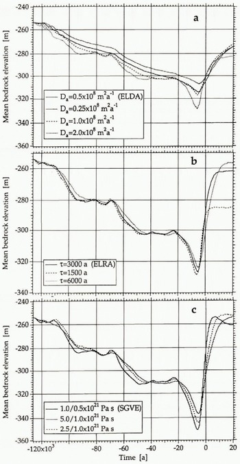
Fig. 4. Sensitivity test on the characteristic parameters for the three most realistic bedrock models: ELDA (a). ELRA (b) and SGVE (c). This demonstrates that, when parameters are varied within their range of uncertainty, the deviations within one method can easily be as much as those obtained from one model to another. Unfortunately, for the present Antarctic ice sheet, there is little observational evidence available to check the validity of the respective results.
6. Conclusion
In this paper, we have discussed ways of dealing with isostasy in ice-sheet models and have compared the results of five methods applied to a simulation of the Antarctic ice sheet during the last glacial cycle. A first point to mention is that the bedrock response has to be taken into account to be able to reproduce the final deglaciation within a realistic range of the climatic-forcing parameters. All bedrock models have in common the fact that parameters can always be selected within their range of uncertainty to model satisfactorily the large-scale characteristics of a complete cycle of growth and retreat. Therefore, as long as these parameters cannot be constrained better and as long as the interest is in the global ice-sheet evolution, it is difficult to discriminate between the various bedrock parameterizations.
However, when interest is in accurate geometrical patterns, it becomes possible to favour or discard some of the models. In this respect, the LLDA model (local lithosphere, diffusive asthenosphere) clearly performed worst, regarding both the spatial and the time-dependent aspects of the response. The LL treatment caused the effect of the load to be concentrated too much and the DA model was shown to be inherently deficient. The LLDA method happens to be the most commonly used one in ice-sheet models but it also has the largest limitations.
It has finally turned out that the set of acceptable models reduced to the full Earth model (SGVE) and, if a choice has to be made, also to the ELRA model (elastic lithosphere, relaxed asthenosphere). The latter model has the great advantage of being more suitable in terms of coding and computer requirements, while at the same time being able to reproduce the most important characteristics common to the SGVE model. The drawback is that only one time constant can be considered. Nevertheless, in the study of features that are very sensitive to slight bedrock changes, such as the process of grounding-line migration, it is obvious that the most accurate available bedrock model is also the most appropriate. For that purpose, full Earth models like that described in the present paper should be used, provided that the corresponding extra costs can be managed. Here, the degree of confidence arises from a basically correct treatment of the physics and from the ability of such models to reproduce post-glacial rebound patterns as revealed by field measurements (Lambeck and others, 1990; Peltier, 1991a; Fjeldskaar, 1994; Le Meur, 1996). Realistic as they may seem, however, these full Earth isostasy models are also strongly dependent on the Earth parameters they require as input. The guarantee for reliable results then requires a correct knowledge of these properties but unfortunately the two key parameters, which are the lithospheric thickness and the viscosity profile within the mantle, remain uncertain.
Acknowledgements
The authors are particularly grateful to the European Science Foundation which provided E. Le Meur with an EISMINT exchange grant and allowed several visits to the Alfred-Wegener-Institut (AWI) in the context of this paper. E. Le Meur would also like to thank P. Godefroy, Bureau de Recherches Géologiques et Minières, Marseilles, whose help in funding a previous 16 months’ stay at AWI has been decisive in the development of the full Earth bedrock model presented here. During this research, P. Huybrechts was on leave front the Belgian National Fund for Scientific Research (NFWO). This is AWI Contribution No. 959.


