


1. Introduction
Inherently non-equilibrium suspensions of active particles abound in biological and experimental settings (Marchetti et al. Reference Marchetti, Joanny, Ramaswamy, Liverpool, Prost, Rao and Simha2013; Gompper et al. Reference Gompper2020). For example, motile bacteria such as E. coli and Bacillus subtilis propel themselves through their surrounding fluid environment, interacting through their induced flow fields (Pedley & Kessler Reference Pedley and Kessler1992; Mendelson et al. Reference Mendelson, Bourque, Wilkening, Anderson and Watkins1999; Lauga & Powers Reference Lauga and Powers2009; Lushi, Wioland & Goldstein Reference Lushi, Wioland and Goldstein2014), while likewise immersed microtubule bundles slide and extend, driven by ATP-driven molecular motors (Sanchez et al. Reference Sanchez, Chen, DeCamp, Heymann and Dogic2012; Henkin et al. Reference Henkin, DeCamp, Chen, Sanchez and Dogic2014; DeCamp et al. Reference DeCamp, Redner, Baskaran, Hagan and Dogic2015; Needleman & Dogic Reference Needleman and Dogic2017; Opathalage et al. Reference Opathalage, Norton, Juniper, Langeslay, Aghvami, Fraden and Dogic2019). These active suspensions are remarkable because, despite the near lack of inertial effects relative to viscous ones, the activity of the particles can produce large-scale coherent flows and even so-called active or bacterial turbulence, characterized by chaotic fluctuations in particle concentration and fluid velocity (Simha & Ramaswamy Reference Simha and Ramaswamy2002; Dombrowski et al. Reference Dombrowski, Cisneros, Chatkaew, Goldstein and Kessler2004; Sokolov et al. Reference Sokolov, Aranson, Kessler and Goldstein2007; Zhang et al. Reference Zhang, Be'er, Florin and Swinney2010; Koch & Subramanian Reference Koch and Subramanian2011; Sokolov & Aranson Reference Sokolov and Aranson2012; Dunkel et al. Reference Dunkel, Heidenreich, Drescher, Wensink, Bär and Goldstein2013; Gachelin et al. Reference Gachelin, Rousselet, Lindner and Clement2014; Thampi, Golestanian & Yeomans Reference Thampi, Golestanian and Yeomans2014; Doostmohammadi et al. Reference Doostmohammadi, Shendruk, Thijssen and Yeomans2017; Nishiguchi et al. Reference Nishiguchi, Nagai, Chaté and Sano2017; Stenhammar et al. Reference Stenhammar, Nardini, Nash, Marenduzzo and Morozov2017; Peng, Liu & Cheng Reference Peng, Liu and Cheng2021).
Here, we consider the kinetic model for a dilute suspension of active elongated particles developed by Saintillan and Shelley (Saintillan & Shelley Reference Saintillan and Shelley2008a,Reference Saintillan and Shelleyb). We note that a similar model was developed independently by Subramanian & Koch (Reference Subramanian and Koch2009), and that both models share many similarities with the Doi–Edwards model for passive polymers (Doi Reference Doi1981; Doi & Edwards Reference Doi and Edwards1986). In the dilute limit, particles interact with each other hydrodynamically only by exerting an ‘active stress’ on the surrounding fluid. Even in this setting, changes in particle density and activity are known to cause the suspension to transition from a uniform isotropic state to more complex states – many of which are observed experimentally – involving large-scale patterns in particle alignment and concentration. The kinetic model (Saintillan & Shelley Reference Saintillan and Shelley2008a,Reference Saintillan and Shelleyb) thus presents an opportunity to elucidate some of the fundamental mechanisms behind the transition to collective dynamics and active turbulence.
To understand this transition, we perform a multiple time scales expansion to determine exactly how the uniform isotropic steady state in the two-dimensional (2-D) kinetic model loses stability in different parameter regimes. The variety of predicted behaviours near the onset of instability, which we verify through numerical simulations, is surprisingly complex. Linear stability analysis alone shows that, depending on the (fixed) ratio of particle diffusivity to concentration, the uniform isotropic state can lose stability through either a pitchfork or Hopf bifurcation. Here, the bifurcation parameter is a ratio of the particle swimming speed to the particle concentration and magnitude of active stress that the particles exert. Our weakly nonlinear analysis shows that both the pitchfork and Hopf parameter regions can be subdivided further into subcritical and supercritical regions, again depending on the ratio of particle diffusivity to concentration.
Numerically, we find hysteresis in the subcritical Hopf region, where far-from-isotropic quasi-periodic patterns of particle alignment are bistable with the uniform isotropic state. The patterns in this region are perhaps precursors to active turbulence. However, the dimensionality of the initial perturbation to the isotropic steady state makes a difference. If the initial perturbation is one-dimensional (1-D), i.e. purely in the  $x$- or $y$-direction, then only a supercritical Hopf bifurcation can occur, and we locate numerically the stable limit cycle that arises. An example of a 2-D limit cycle is also located numerically within the region in which both 1-D and 2-D perturbations give rise to a supercritical Hopf bifurcation. In the supercritical pitchfork setting, which includes immotile (but active) particles, we identify the stable steady states emerging just beyond the bifurcation. These steady states resemble the steady vortex found in Wioland et al. (Reference Wioland, Woodhouse, Dunkel, Kessler and Goldstein2013), although we consider periodic boundary conditions rather than confinement.
A key takeaway is that even this simple kinetic model is capable of capturing many different types of transitions to collective behaviour in an active suspension. The different bifurcations analysed here can be compared with systematic numerical studies of phase transitions in other active suspension models (Forest, Wang & Zhou Reference Forest, Wang and Zhou2004a,Reference Forest, Wang and Zhoub; Giomi et al. Reference Giomi, Mahadevan, Chakraborty and Hagan2011, Reference Giomi, Mahadevan, Chakraborty and Hagan2012; Xiao-Gang, Forest & Qi Reference Xiao-Gang, Forest and Qi2014; Yang, Marenduzzo & Marchetti Reference Yang, Marenduzzo and Marchetti2014) and help to explain the 1-D and 2-D patterns – including limit cycles and other attractors – located numerically in Forest et al. (Reference Forest, Phuworawong, Wang and Zhou2014) and Forest, Wang & Zhou (Reference Forest, Wang and Zhou2013, Reference Forest, Wang and Zhou2015) for a similar version of the kinetic model. The weakly nonlinear analysis performed here also facilitates comparison with the normal forms arising in more classical pattern formation processes in fluid mechanics, especially thermal convection (Swift & Hohenberg Reference Swift and Hohenberg1977; Swinney & Gollub Reference Swinney and Gollub1981; Knobloch Reference Knobloch1986; Pomeau Reference Pomeau1986; Crawford & Knobloch Reference Crawford and Knobloch1991; Cross & Hohenberg Reference Cross and Hohenberg1993; Schöpf & Zimmermann Reference Schöpf and Zimmermann1993), but also other phenomena arising in complex fluids such as electrohydrodynamic convection in nematic liquid crystals (Bodenschatz, Zimmermann & Kramer Reference Bodenschatz, Zimmermann and Kramer1988) and the transition from subcritical to supercritical instability in viscoelastic pipe flow (Wan, Sun & Zhang Reference Wan, Sun and Zhang2021).
The paper begins by introducing the kinetic model (§ 2.1) and recapping the well-studied linear stability analysis (§§ 2.2, 2.3) and role of rotational diffusion (§ 2.4). Readers familiar with the model may wish to skip directly to the outline of results in § 2.5, where the types of bifurcations are mapped out in greater detail.
2. Background
2.1. Kinetic model of an active suspension
In the kinetic model (Saintillan & Shelley Reference Saintillan and Shelley2008a,Reference Saintillan and Shelleyb), a suspension of  $N$ elongated particles in a 2-D periodic box of length $L$ is modelled as a number density $\varPsi (\boldsymbol {x},\boldsymbol {p},t)$ of particles with centre-of-mass position $\boldsymbol {x}$ and orientation $\boldsymbol {p}\in S^{1}$ at time $t$. Due to conservation of the number of particles, the density $\varPsi$ evolves according to a Smoluchowski equation:
 \begin{equation} {\partial}_t \varPsi ={-}\boldsymbol{\nabla}\boldsymbol{\cdot}(\dot{\boldsymbol{x}}\varPsi) - \boldsymbol{\nabla}_p\boldsymbol{\cdot}(\dot{\boldsymbol{p}}\varPsi), \quad \boldsymbol{\nabla}_p := ({\boldsymbol I} -\boldsymbol{p}\boldsymbol{p}^{\rm T})\,{\partial}_{\boldsymbol{p}}. \end{equation}
Here,  $\boldsymbol {\nabla }_p\boldsymbol {\cdot }$ denotes the divergence on the unit sphere. The translational and rotational fluxes are given by
 $$\begin{gather} \dot{
\boldsymbol{x}} = V_0\boldsymbol{p} + \boldsymbol{u} -
D_T\,\boldsymbol{\nabla}(\log \varPsi),
\end{gather}$$
$$\begin{gather} \dot{
\boldsymbol{x}} = V_0\boldsymbol{p} + \boldsymbol{u} -
D_T\,\boldsymbol{\nabla}(\log \varPsi),
\end{gather}$$ $$\begin{gather}\dot{\boldsymbol{p}} = ({\boldsymbol I}-\boldsymbol{p}\boldsymbol{p}^{\rm T})(\boldsymbol{\nabla} \boldsymbol{u} \boldsymbol{p}) - D_R\,\boldsymbol{\nabla}_p(\log \varPsi). \end{gather}$$
The translational velocity consists of a particle swimming term with speed  $V_0$ in direction $\boldsymbol {p}$, particle advection by the surrounding fluid flow, and translational diffusion. For simplicity, we take the translational diffusion to be isotropic. The rotational velocity depends on a Jeffery term for the rotation of an elongated particle in Stokes flow (Jeffery Reference Jeffery1922), written here in the infinitely slender limit, along with rotational diffusion.
Finally, the surrounding fluid medium satisfies the Stokes equations with active forcing:
 $$\begin{gather} -\mu\,{\rm \Delta} \boldsymbol{u} + \boldsymbol{\nabla} q = \boldsymbol{\nabla}\boldsymbol{\cdot} {\boldsymbol \varSigma}^{a},\quad \boldsymbol{\nabla}\boldsymbol{\cdot}\boldsymbol{u} =0, \end{gather}$$
 $$\begin{gather}{\boldsymbol \varSigma}^{a} = a_0 \int_{S^{1}} \varPsi(\boldsymbol{x},\boldsymbol{p},t)\left(\boldsymbol{p}\boldsymbol{p}^{\rm T}- \tfrac{1}{2}{\boldsymbol I}\right){\rm d}\boldsymbol{p}. \end{gather}$$
Here,  $\boldsymbol {u}(\boldsymbol {x},t)$ and $q(\boldsymbol {x},t)$ are the fluid velocity and pressure, $\mu$ is the fluid viscosity, and ${\boldsymbol \varSigma }^{a}(\boldsymbol {x},t)$ is the trace-free active stress exerted by the particles on the fluid. The active stress is the orientational average of the force dipoles exerted by the particles on the fluid, and the sign of the coefficient $a_0$ corresponds to the sign of the dipoles: $a_0>0$ for puller particles, while $a_0<0$ for pushers. Note that ${\boldsymbol \varSigma }^{a}$ vanishes when the particles are in complete nematic alignment.
2.2. Non-dimensionalization and quantities of interest
We choose to non-dimensionalize (2.1a,b)–(2.5) over slightly different characteristic velocity, length and time scales from those used commonly in the literature (Saintillan & Shelley Reference Saintillan and Shelley2008a,Reference Saintillan and Shelleyb; Hohenegger & Shelley Reference Hohenegger and Shelley2010; Ezhilan, Shelley & Saintillan Reference Ezhilan, Shelley and Saintillan2013). In particular, letting  $N$ denote the number of particles in the system and $L$ denote the length of the periodic box in which the particles are suspended, we non-dimensionalize the model (2.1a,b)–(2.5) according to
 \begin{equation} \varPsi'= \frac{\varPsi}{N/L^{2}}, \quad \boldsymbol{x}' = \frac{\boldsymbol{x}}{L/2{\rm \pi}}, \quad t' = \frac{|a_0| N}{L^{2}\mu}\,t,\quad \boldsymbol{u}' = \frac{2{\rm \pi}\mu L}{|a_0| N}\,\boldsymbol{u}, \end{equation}
which results in the following system of equations:
 \begin{equation} \left.\begin{gathered} {\partial}_{t'} \varPsi' ={-}{\rm{div}}'({\partial}_{t'}\boldsymbol{x}'\varPsi') - \boldsymbol{\nabla}_p({\partial}_{t'}\boldsymbol{p}\varPsi'), \\ {\partial}_{t'} \boldsymbol{x}' = \beta\boldsymbol{p} + \boldsymbol{u}' - D_T'\,\boldsymbol{\nabla}'(\log \varPsi'), \\ {\partial}_{t'} \boldsymbol{p} = (\boldsymbol{I}-\boldsymbol{p}\boldsymbol{p}^{\rm T})(\boldsymbol{\nabla}' \boldsymbol{u}' \boldsymbol{p}) - D_R'\,\boldsymbol{\nabla}_p(\log \varPsi'), \\ -{\rm \Delta}' \boldsymbol{u}' + \boldsymbol{\nabla}' q' ={\pm} \int_{S^{1}} \left(\boldsymbol{p}\boldsymbol{p}^{\rm T}- \tfrac{1}{2}\boldsymbol{I}\right)\boldsymbol{\nabla}'\varPsi'(\boldsymbol{x},\boldsymbol{p},t)\,{\rm d}\boldsymbol{p}, \quad {\rm{div}}'\boldsymbol{u}' =0. \end{gathered}\right\} \end{equation}
Here, we note the presence of three dimensionless parameters: the diffusion coefficients
 \begin{equation} D_T' = \frac{4{\rm \pi}^{2} \mu D_T}{\left\lvert a_0 \right\rvert N} \quad \text{and} \quad D_R' = \frac{\mu L^{2} D_R}{\left\lvert a_0 \right\rvert N}, \end{equation}
and a non-dimensional ‘swimming speed’
 \begin{equation} \beta= \frac{2{\rm \pi}\mu V_0 L}{\left\lvert a_0 \right\rvert N}. \end{equation}
We choose this non-dimensionalization in order to incorporate easily the immotile state ( $V_0=0$) into the analysis. Without swimming, (2.1a,b)–(2.5) describe a suspension of shakers (Ezhilan et al. Reference Ezhilan, Shelley and Saintillan2013; Stenhammar et al. Reference Stenhammar, Nardini, Nash, Marenduzzo and Morozov2017), particles that do not swim but still exert an active stress on the surrounding fluid. We also fix the domain to be the 2-D torus $\mathbb {T}^{2}:=\mathbb {R}^{2}/(2{\rm \pi} \mathbb {Z})^{2}$.
The parameter  $\beta$ contains more information than just the particle swimming speed: it is really the ratio of swimming speed to the active stress magnitude and particle concentration. Note that $\beta$ may be related to the more familiar non-dimensionalization used in Hohenegger & Shelley (Reference Hohenegger and Shelley2010) and Saintillan & Shelley (Reference Saintillan and Shelley2008b) via $\beta = (2{\rm \pi} \ell )/(|\alpha |\,L\nu )$, where $\ell$ is the length of typical swimmer, $\alpha =a_0/(V_0\mu \ell )$ is a dimensionless signed active stress coefficient ( $\alpha >0$ for pullers and $\alpha <0$ for pushers), and $\nu =N\ell ^{2}/L^{2}$ is the relative volume concentration of swimmers.
In (2.7), the active stress coefficient in the Stokes equations is scaled to unit magnitude but retains the sign of the force dipole exerted by the particles on the fluid:  $+1$ for puller particles, and $-1$ for pusher particles.
Dropping the prime notation, the system (2.7) may be written more succinctly as
 \begin{align} \left.\begin{gathered} {\partial}_t \varPsi ={-}\beta \boldsymbol{p}\boldsymbol{\cdot}\boldsymbol{\nabla}\varPsi -\boldsymbol{u}\boldsymbol{\cdot}\boldsymbol{\nabla}\varPsi -{{\rm div}}_p\left((\boldsymbol{I}-\boldsymbol{p}\boldsymbol{p}^{\rm T})(\boldsymbol{\nabla}\boldsymbol{u}\boldsymbol{p})\varPsi \right) + D_T\,{\rm \Delta} \varPsi +D_R\,{\rm \Delta}_p\varPsi, \\ -{\rm \Delta} \boldsymbol{u} + \boldsymbol{\nabla} q ={\pm} \int_{S^{1}} \left(\boldsymbol{p}\boldsymbol{p}^{\rm T}- \tfrac{1}{2}\boldsymbol{I}\right)\boldsymbol{\nabla} \varPsi(\boldsymbol{x},\boldsymbol{p},t)\,{\rm d}\boldsymbol{p}, \quad {\rm{div}}\,\boldsymbol{u} =0 . \end{gathered}\right\} \end{align}
 One way to measure deviations of the swimmer density  $\varPsi$ from the uniform isotropic steady state $\varPsi _0=1/(2{\rm \pi} )$ is to consider the relative entropy
 \begin{equation} \mathcal{S}(t) = \int_{\mathbb{T}^{2}}\int_{S^{1}} \frac{\varPsi}{\varPsi_0}\log \left(\frac{\varPsi}{\varPsi_0} \right) \,{\rm d}\boldsymbol{p}\,{\rm d}\boldsymbol{x}. \end{equation}
Using (2.10), the entropy can be shown to evolve according to
 \begin{align} \dot {\mathcal{S}}(t) ={\mp} \frac{4}{\varPsi_0}\int_{\mathbb{T}^{2}} \left\lvert \boldsymbol{\mathsf{E}} \right\rvert^{2}{\rm d}\boldsymbol{x} - \int_{\mathbb{T}^{2}}\int_{S^{1}} \left( D_T\left\lvert \boldsymbol{\nabla}(\log\varPsi) \right\rvert^{2} + D_R \left\lvert \boldsymbol{\nabla}_p(\log(\varPsi)) \right\rvert^{2} \right) \frac{\varPsi}{\varPsi_0}\,{\rm d}\boldsymbol{p} \,{\rm d}\boldsymbol{x}, \end{align}
where  $\boldsymbol{\mathsf{E}}= \frac {1}{2}(\boldsymbol {\nabla }\boldsymbol {u}+(\boldsymbol {\nabla }\boldsymbol {u})^\textrm {T})$ (see Saintillan & Shelley Reference Saintillan and Shelley2008b). The first term in (2.12) arises from the viscous dissipation of the active stress exerted by the particles, and is negative for pullers and positive for pushers. The two diffusive terms are negative; hence we expect puller suspensions to always relax to isotropy over time. For pushers, however, we may expect to see some more interesting behaviours: indeed, simulations show that patterns and fluctuations in particle alignment and concentration arise in certain parameter regimes (Saintillan & Shelley Reference Saintillan and Shelley2008a,Reference Saintillan and Shelleyb, Reference Saintillan and Shelley2013, Reference Saintillan and Shelley2015; Hohenegger & Shelley Reference Hohenegger and Shelley2010). We aim to study the onset of pattern formation in these active pusher suspensions.
It will be useful to first define some system quantities that can be measured numerically and used to verify analytical predictions. One such quantity is the active power input, defined for pusher particles by
 \begin{equation} \mathcal{P}(t) = \int_{\mathbb{T}^{2}} \int_{S^{1}} \boldsymbol{p}^{\rm T}\,\boldsymbol{\mathsf{E}}(\boldsymbol{x},t)\,\boldsymbol{p}\,\varPsi(\boldsymbol{x},\boldsymbol{p},t)\,{\rm d}\boldsymbol{p} \,{\rm d}\boldsymbol{x}. \end{equation}
The sign is opposite for puller particles. This quantity can be understood as the perturbative power input due to the interaction of the active particles with the flow (as opposed to the power input of each individual particle). Using the Stokes equations in (2.10), the active power balances the rate of viscous dissipation in the fluid:
 \begin{equation} \mathcal{P}(t) = \int_{\mathbb{T}^{2}} 2 \left\lvert \boldsymbol{\mathsf{E}}(\boldsymbol{x},t) \right\rvert^{2}{\rm d}\boldsymbol{x}. \end{equation}
Note that  $\mathcal {P}(t)=0$ for the uniform isotropic steady state, and tracking the growth of $\mathcal {P}(t)$ (or, equivalently, the rate of viscous dissipation) serves as a measure of the instability of the uniform state (Saintillan & Shelley Reference Saintillan and Shelley2015).
We also define the concentration field
 \begin{equation} c(\boldsymbol{x},t) = \int_{S^{1}}\varPsi(\boldsymbol{x},\boldsymbol{p},t)\,{\rm d}\boldsymbol{p} \end{equation}
and the nematic order tensor
 \begin{equation} \boldsymbol{\mathsf{Q}}(\boldsymbol{x},t) = \frac{1}{c(\boldsymbol{x},t)}\int_{S^{1}}(\boldsymbol{p}\boldsymbol{p}^{\rm T}-\boldsymbol{I}/2)\, \varPsi(\boldsymbol{x},\boldsymbol{p},t)\,{\rm d}\boldsymbol{p} . \end{equation}
We can then define the scalar-valued nematic order parameter as
 \begin{equation} \mathcal{N}(\boldsymbol{x},t) = \text{maximum eigenvalue of }\boldsymbol{\mathsf{Q}}(\boldsymbol{x},t). \end{equation}
The nematic order parameter measures the local degree of nematic alignment:  ${\mathcal{N}(\boldsymbol{x},t)=0}$ when the particle orientations are isotropic, and $\mathcal {N}(\boldsymbol {x},t)=1$ when all surrounding particles are exactly aligned.
2.3. Linear stability: the eigenvalue problem
From here, we restrict our attention to the pusher case in two spatial dimensions. We begin by recalling the results of the eigenvalue problem resulting from a linear stability analysis about the uniform isotropic steady state  $\varPsi _0=1/(2{\rm \pi} )$ and $\boldsymbol {u}=0$ (Saintillan & Shelley Reference Saintillan and Shelley2008b; Hohenegger & Shelley Reference Hohenegger and Shelley2010; Subramanian, Koch & Fitzgibbon Reference Subramanian, Koch and Fitzgibbon2011). Linearizing (2.10) about this state, we obtain
 \begin{equation} \left.\begin{gathered} {\partial}_t \varPsi ={-} \beta\boldsymbol{p}\boldsymbol{\cdot}\boldsymbol{\nabla}\varPsi + 2 \boldsymbol{p}^{\rm T}\,\boldsymbol{\nabla}\boldsymbol{u} \boldsymbol{p} + D_T\,{\rm \Delta} \varPsi + D_R\,{\rm \Delta}_p\varPsi, \\ - {\rm \Delta} \boldsymbol{u} + \boldsymbol{\nabla} q ={-}\displaystyle\frac{1}{2{\rm \pi}} \int_{S^{1}} \left(\boldsymbol{p}\boldsymbol{p}^{\rm T}- \frac{1}{2}\boldsymbol{I}\right)\boldsymbol{\nabla} \varPsi(\boldsymbol{x},\boldsymbol{p},t) \,{\rm d}\boldsymbol{p}, \quad {\rm{div}}\,\boldsymbol{u} =0. \end{gathered}\right\} \end{equation}
 We insert the plane wave ansatz  $\varPsi = \psi (\boldsymbol {k},\boldsymbol {p})\exp ({\textrm {i}\boldsymbol {k}\boldsymbol {\cdot }\boldsymbol {x}+\sigma t})$, $\sigma \in \mathbb {C}$, into (2.18), and choose coordinates such that the wave vector is $\boldsymbol {k} = k\boldsymbol {e}_x$ and the particle orientation is $\boldsymbol {p} = \cos \theta \,\boldsymbol {e}_x+\sin \theta \,\boldsymbol {e}_y$, $0\le \theta <2{\rm \pi}$. Defining $\lambda _k:= \sigma + D_Tk^{2}$, we obtain an eigenvalue problem for $\lambda _k$ in the form of an integrodifferential equation on $S^{1}$:
 \begin{align} \lambda_k\,\psi(k,\theta) &={-}{\rm i}k\beta\cos\theta\,\psi(k,\theta) \nonumber\\ &\quad +\frac{1}{\rm \pi} \cos\theta\sin\theta \int_0^{2{\rm \pi}}\psi(k,\theta) \sin\theta\cos\theta \,{\rm d}\theta + D_R\,{\partial}_{\theta\theta} \psi(k,\theta). \end{align}
 We note that while it may be more suggestive to write  $\psi$ in terms of $\sin (2\theta )$ rather than $\sin \theta \cos \theta$, we find that the details of the weakly nonlinear calculations in the following sections are slightly simpler in terms of $\cos \theta =\boldsymbol {p}\boldsymbol {\cdot }\boldsymbol {e}_x$ and $\sin \theta =\boldsymbol {p}\boldsymbol {\cdot }\boldsymbol {e}_y$ only.
In the absence of rotational diffusion ( $D_R=0$), we may solve (2.19) for $\psi (k,\theta )$ as
 \begin{equation} \psi(k,\theta) = \frac{\cos\theta\sin\theta}{\lambda_k+{\rm i}k\beta\cos\theta}, \end{equation}
where  $\lambda _k$ is such that
 \begin{equation} F[\psi]:=\int_0^{2{\rm \pi}}\psi(k,\theta)\cos\theta\sin\theta\,{\rm d}\theta = {\rm \pi}. \end{equation}
In particular,  $\lambda _k$ satisfies the implicit dispersion relation
 \begin{equation} \frac{\lambda_k\beta^{2}k^{2}+2\lambda_k^{3} - 2\lambda_k^{2}\sqrt{\beta^{2}k^{2}+\lambda_k^{2}}}{\beta^{4}k^{4}} = 1. \end{equation}
 Recalling that  $\lambda _k = \sigma +D_Tk^{2}$, we may then solve numerically for the relationship between $\sigma$ and $\beta$ (see figure 1).

Figure 1. (a) Real part (shifted by  $D_Tk^{2}$) and (b) imaginary part of the growth rate $\sigma (k)$ versus $\beta \left \lvert k \right \rvert$. Plot (a) can be read as follows. Fix a value of $0< D_Tk^{2}<0.25$. Look at the corresponding horizontal green line. As $\beta$ is lowered, the green line intersects the blue curve. This is where the eigenvalue $\sigma (k)$ becomes unstable. Different types of bifurcations are possible depending on the value of $D_Tk^{2}$: for example, point B corresponds to a purely real eigenvalue crossing, while the presence of non-zero $\textrm {Im}(\sigma )$ signals a Hopf bifurcation at points D and E. At point C, indicated by a red dot, two real eigenvalues meet and become complex. In the case of shakers ( $\beta =0$), we may consider the real eigenvalue crossing at point A along the $y$-axis.
A similar calculation for  $\boldsymbol {k}=k\boldsymbol {e}_y$ shows that the eigenvalues $\sigma (k)$ plotted in figure 1 also correspond to a $y$-direction eigenfunction whose eigenmodes are a $90^{\circ }$ rotation (in $\theta$) of the $x$-direction eigenmodes. The solutions of (2.18) arising from eigenfunctions of the linearized operator are thus given by
 \begin{align} \varPsi(\boldsymbol{x},\theta,t) = c_x\,\psi_x(k,\theta)\exp({{\rm i}kx+\sigma t}) +c_y\, \psi_y(k,\theta)\exp({{\rm i}ky+\sigma t}), \quad c_x^{2}+c_y^{2}=1, \end{align}
and all scalar multiples of (2.23), where
 \begin{equation} \psi_x(k,\theta) = \frac{\cos\theta\sin\theta}{\sigma+D_Tk^{2}+{\rm i}k\beta\cos\theta},\quad \psi_y(k,\theta) = \frac{\cos\theta\sin\theta}{\sigma+D_Tk^{2}+{\rm i}k\beta\sin\theta}. \end{equation}
In particular, besides point C, each eigenvalue  $\sigma (k)$ has a four-dimensional eigenspace over $\mathbb {C}$, spanned by the $x$- and $y$-direction components with $\pm k$. When ${\beta \left \lvert k \right \rvert <\sqrt {3}/9}$, there are two distinct real-valued eigenvalues $\sigma (k)$ that satisfy the required condition $\int _0^{2{\rm \pi} }\psi _x \cos \theta \sin \theta \, \textrm {d}\theta =\int _0^{2{\rm \pi} }\psi _y \cos \theta \sin \theta \,\textrm {d}\theta ={\rm \pi}$, both of which then have a four-dimensional eigenspace over $\mathbb {R}$.
Note that the dispersion relation (2.22) is exact only in the absence of rotational diffusion, but for the purposes of this paper, we will consider  $0< D_R\ll 1$. This alters figure 1, but only slightly (see § 2.4 for details). In return, we do not have to contend with the continuous spectrum present in the $D_R=0$ spectral analysis of Subramanian et al. (Reference Subramanian, Koch and Fitzgibbon2011). Furthermore, when $D_R>0$, the $k=0$ mode is always linearly stable, as it satisfies the heat equation in $\boldsymbol {p}$: if $\varPsi =\varPsi (\boldsymbol {p},t)$, then $ {\partial }_t\varPsi =D_R\,{\rm \Delta} _p\varPsi$.
The eigenvalue relation (2.22) ceases to be valid for  $\textrm {Re}(\lambda _k)\le 0$, i.e. when $\textrm {Re}(\sigma (k))\le -D_Tk^{2}$ (Hohenegger & Shelley Reference Hohenegger and Shelley2010; Subramanian et al. Reference Subramanian, Koch and Fitzgibbon2011). For fixed $0< D_T<1/4$, however, the eigenvalue analysis does capture a sign change in the real part of the growth rate $\sigma (k)$ as $\beta \left \lvert k \right \rvert$ is varied. For each $k$, this sign change occurs where the blue curve in figure 1 (corresponding to $\lambda _k$) intersects the green line corresponding to the fixed value of $D_Tk^{2}$. Numerical simulations indicate that if the point $(D_Tk^{2},\beta \left \lvert k \right \rvert )$ lies to the right of the blue contour in figure 1(a) for each $k$, then the uniform isotropic steady state is stable to small perturbations (see §§ 4 and 5). In this region, particle diffusion and swimming – processes that tend to decrease order among the particles – are large relative to both the active stress magnitude and the particle concentration, which favour local alignment. As $\beta$ is decreased, $\textrm {Re}(\sigma (k))$ crosses the green line corresponding to the (fixed) value of $D_Tk^{2}$, and the uniform isotropic state becomes unstable.
Since we are considering the system (2.7) on a periodic domain and have non-dimensionalized  $\boldsymbol {x}$ according to the length of the domain, the $\left \lvert k \right \rvert =1$ mode is the lowest non-trivial mode in the system and hence the first to lose stability as $\beta$ decreases. As noted in Koch & Subramanian (Reference Koch and Subramanian2011), ‘the finiteness of the domain may act to stabilize the system’. Indeed, the stabilizing effects of mixing on $\mathbb {T}^{d}$ ( $d=2,3$) due to swimming are studied in Albritton & Ohm (Reference Albritton and Ohm2022) and play a role in the patterns observed here.
We aim to understand the onset of pattern formation in (2.7) by exploring the many different ways in which the  $\left \lvert k \right \rvert =1$ mode can lose stability as $\beta$ is decreased. From figure 1, we can see that depending on $D_T$, the type of bifurcation that we expect to see for the $\left \lvert k \right \rvert =1$ mode will change. We aim to characterize all of the types of initial bifurcations admitted by the system through a weakly nonlinear analysis. According to the dispersion relation, if $1/9< D_T<1/4$, as $\beta$ decreases, the purely real eigenvalue $\sigma$ will change sign from positive to negative across the top branch of the blue curve, between points A and C. For $0< D_T<1/9$, however, we expect to see a Hopf bifurcation as $\beta$ crosses the blue curve roughly between points C and E, since for these values of $\beta$, $\sigma$ has non-zero imaginary part.
As noted, figure 1 does not quite give the exact locations of the bifurcations that we will consider here, since we still need to consider the effects of (small)  $D_R>0$. This will be the subject of the next subsection.
2.4. Role of rotational diffusion
The dispersion relation (2.22) was obtained in the absence of rotational diffusion; however, studying pattern formation near the isotropic steady state will require  $D_R>0$. When $D_R=0$, the system (2.10) has infinitely many steady states; in particular, any spatially uniform swimmer distribution $\varPsi =\varPsi (\boldsymbol {p})$ is a steady state. The continuum of nearby steady states obscures the mechanism by which the isotropic state $\varPsi =1/(2{\rm \pi} )$ loses stability; indeed, any function $\varPsi (\boldsymbol {p})$ belongs to the kernel of the linearized operator. When we add in $D_R>0$ (along with the assumption that the total number of swimmers is conserved), this kernel is eliminated. Thus we aim to determine when the effect of small $D_R>0$ can be considered as a perturbation of the dispersion relation (2.22) and figure 1.
In particular, given a wavenumber  $k$, for small $D_R>0$, we wish to determine when an expansion (in $D_R$) of the form
 \begin{equation} \sigma = \sigma_0 + D_R\sigma_1 + O(D_R^{2}),\quad \psi = \psi_0 + D_R \psi_1 + O(D_R^{2}) \end{equation}
is valid for some  $(\sigma _1,\psi _1)$.
Plugging this expansion into the eigenvalue problem (2.19) and separating scales, at  $O(1)$ we obtain the $D_R=0$ eigenfunctions and eigenvalue relation
 \begin{equation} \psi_0(k,\theta) = \frac{\cos\theta\sin\theta}{\sigma_0+D_Tk^{2}+{\rm i}k\beta\cos\theta}, \end{equation}
where  $\sigma _0$ is such that
 \begin{equation} F[\psi_0]=\int_0^{2{\rm \pi}}\psi_0\cos\theta\sin\theta \,{\rm d}\theta= {\rm \pi}. \end{equation}
 At  $O(D_R)$, we obtain the expression
 \begin{align} \psi_1 &= \frac{1}{\rm \pi}\psi_0\int_0^{2{\rm \pi}} \psi_1\cos\theta'\sin\theta' \,{\rm d}\theta' \nonumber\\ &\quad -\frac{\sigma_1\psi_0}{\sigma_0+D_Tk^{2}+{\rm i}k\beta\cos\theta} + \frac{{\partial}_\theta^{2}\psi_0}{\sigma_0+D_Tk^{2}+{\rm i}k\beta\cos\theta}. \end{align}
Taking  $F[\boldsymbol {\cdot }]$ of both sides and using (2.27) then yields an integral expression for $\sigma _1$:
 \begin{equation} \sigma_1 \int_0^{2{\rm \pi}}\frac{\cos^{2}\theta\sin^{2}\theta}{(\sigma_0+D_Tk^{2}+{\rm i}k\beta\cos\theta)^{2}}\,{\rm d}\theta = \int_0^{2{\rm \pi}}\frac{{\partial}_\theta^{2}\psi_0 \cos\theta\sin\theta}{\sigma_0+D_Tk^{2}+{\rm i}k\beta\cos\theta}\,{\rm d}\theta. \end{equation}
As long as  $\textrm {Re}(\sigma _0+D_Tk^{2})\neq 0$ (which holds for the $\left \lvert k \right \rvert =1$ modes as long as $D_T\neq 0$), we obtain an expression for $\sigma _1$:
 \begin{align} \sigma_1 &= \frac{\frac{5}{6}\beta^{2}k^{2}}{\beta^{2}k^{2}-3(D_Tk^{2}+\sigma_0)^{2}} + \frac{\frac{1}{2}\beta^{2}k^{2}}{\beta^{2}k^{2}+(D_Tk^{2}+\sigma_0)^{2}} \nonumber\\ &\quad + \frac{5(D_Tk^{2}+\sigma_0)^{3} }{(\beta^{2}k^{2}-3(D_Tk^{2}+\sigma_0)^{2}) \sqrt{\beta^{2}k^{2}+(D_Tk^{2}+\sigma_0)^{2}}} -\frac{7}{3}, \end{align}
which is finite as long as  $\beta ^{2}k^{2}\neq 3(D_Tk^{2}+\textrm {Re}(\sigma _0))^{2}$. The line
 \begin{equation} \sigma_0+D_Tk^{2}=\frac{\beta \left\lvert k \right\rvert}{\sqrt{3}} \end{equation}
is plotted along with the real part of the  $D_R=0$ dispersion relation (2.22) in figure 2(a). Away from this line, for small $D_R>0$, we may consider the solutions of the eigenvalue problem (2.19) as perturbations of the $D_R=0$ eigenvalues and eigenfunctions. As we can see, this line (2.31) passes through the point C from figure 1 where the two real eigenvalues meet and become two complex conjugate eigenvalues. A very precise choice of $D_T$ and $D_R$ should correspond to a codimension 2 bifurcation at point C; however, a scaling different to (2.25a,b) with respect to $D_R$ is likely needed to study this point in detail. We will not attempt to study point C in detail here, and will instead focus on the more generic bifurcations between points A and C and between points C and E.

Figure 2. The (a) real part and (b) imaginary part of the perturbed dispersion relation  $\sigma _0+D_R\sigma _1$ (dashed black curve) is plotted for $D_R=0.001$ on top of the unperturbed relation with $D_R=0$ (solid light blue curve). The perturbative expression fails to be valid along the grey line $\sigma _0+D_Tk^{2}=\beta \left \lvert k \right \rvert /\sqrt {3}$ plotted in (a). The inset in (a) shows in greater detail the behaviour of the perturbative expression $\sigma _0+D_R\sigma _1$ near the point $(\sqrt {3}/9,1/9)$ where the grey line intersects the unperturbed expression. In particular, the perturbed expression blows up as $\beta \left \lvert k \right \rvert$ approaches $\sqrt {3}/9$.
In figures 2(a) and 2(b), we plot the dispersion relation for  $\sigma _0+D_R\sigma _1$ on top of $\sigma _0$ using $D_R=0.001$. Away from the crossing with the line (2.31), the $\sigma _0+D_R\sigma _1$ curve aligns very closely with the $\sigma _0$ curve. Hereafter, for most numerical purposes, we will take $D_R=0.001$ – small enough to use figure 1 as our roadmap for determining roughly where in the $(D_T,\beta )$ parameter space to look to see different system behaviours. We note that while the expansion in $D_R$ is not rigorous, it is backed later on by the close agreement of the predicted behaviour near bifurcation points (from amplitude equations) with the observed behaviour from numerical simulations. In particular, it appears that away from point C, the small $D_R>0$ picture is largely captured by this expansion.
2.5. Outline of results
The remainder of the paper is devoted to a weakly nonlinear analysis of the different possible bifurcations apparent in figure 1, which we map out in greater detail in figure 3. We begin in § 3 by considering the immotile case  $\beta =0$. We examine the real eigenvalue crossing at point A for all values of $D_R$ for which a bifurcation occurs, and show that the resulting pitchfork bifurcation is always supercritical. In § 4, we assume that $D_R$ is very small and analyse the Hopf bifurcation occurring along the curve between points C and E. We show that for initial perturbations to the uniform isotropic state with both $x$- and $y$-components (i.e. both $c_x, c_y\neq 0$ in (2.23); see line labelled 2-D in figure 3), the bifurcation transitions from supercritical to subcritical at roughly point D, but is always supercritical for initial perturbations with either $c_y=0$ or $c_x=0$ (labelled 1-D in figure 3). In § 5, we again consider very small $D_R$ and study real eigenvalue crossing occurring along the curve between points A and C. The pitchfork bifurcation also transitions from supercritical to subcritical in both the 2-D and 1-D cases, with the change occurring roughly at point B in the case of an initial perturbation in both $x$ and $y$, and just before point C in the case of an $x$-only or $y$-only initial perturbation.

Figure 3. Diagram of the various types of bifurcations through which the uniform isotropic steady state loses stability, depending on the location of the bifurcation value  $\beta _T$. Here, the subscript $T$ is used to reflect that the value of $\beta _T$ depends on the translational diffusion $D_T$ through the dispersion relation plotted in figure 1. Note that the letters A–E correspond to the positions in figure 1(a), which we also repeat here for clarity. The upper line, labelled 2-D, corresponds to the evolution of initial perturbations to the uniform isotropic state with both components in both the $x$- and $y$-directions ( $c_x,c_y\neq 0$ in (2.23)), while the lower line, labelled 1-D, corresponds to perturbations with $x$- or $y$-component only ( $c_y=0$ or $c_x=0$ in (2.23)).
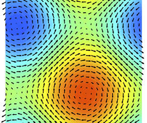
Each section is accompanied by numerical simulations verifying the predicted behaviours near the different bifurcations and illustrating the various states that arise. The numerics are a pseudo-spectral implementation of (2.7) with time stepping via a second-order implicit–explicit backward differentiation scheme.
3. Immotile particles: supercritical pitchfork bifurcation
The simplest scenario for studying the onset of pattern formation in the model (2.10) is in the case  $\beta =0$; i.e. the particles are immotile (or shakers – Ezhilan et al. Reference Ezhilan, Shelley and Saintillan2013; Stenhammar et al. Reference Stenhammar, Nardini, Nash, Marenduzzo and Morozov2017) but still exert a dipolar force on the surrounding fluid. The uniform isotropic steady state in a suspension of immotile particles undergoes a bifurcation to an alignment instability, indicated by point A in figure 1, which we study in greater detail. We first show via weakly nonlinear analysis that the resulting pitchfork bifurcation is always supercritical, and we then explore numerically examples of the emerging non-trivial steady state.
3.1. Weakly nonlinear analysis
In the case of immotile particles, we can calculate explicitly the eigenvalues and eigenfunctions of the linearized operator when  $D_R>0$. The (purely real) eigenvalues $\sigma (k)$ and eigenmodes $\psi _x(k,\theta )$, $\psi _y(k,\theta )$ are given by
 \begin{equation} \sigma(k) = \tfrac{1}{4} - D_Tk^{2} -4D_R, \quad \psi_x(k,\theta)=\psi_y(k,\theta)=\cos\theta\sin\theta. \end{equation}
 From the immotile dispersion relations (3.1a,b), when  $D_T>\frac {1}{4} - 4D_R$, all eigenvalues $\sigma (k)$ are negative, but as $D_T$ is decreased, the $\left \lvert k \right \rvert =1$ modes are the first to change sign as $D_T=D_T^{*} = \frac {1}{4} - 4D_R$ is crossed. We study the nature of this bifurcation for different $D_R$ via the method of multiple scales. For $0<\epsilon \ll 1$, we fix $D_T=\frac {1}{4}-4D_R-\epsilon ^{2}$, so the $\left \lvert k \right \rvert =1$ modes are just barely growing, and define the slow time scale $\tau =\epsilon ^{2} t$. We then assume the following expansions in $\epsilon$:
 \begin{equation} \varPsi = \frac{1}{2{\rm \pi}}(1+\epsilon\varPsi_1 + \epsilon^{2}\varPsi_2 +\epsilon^{3}\varPsi_3 +\cdots),\quad \boldsymbol{u} = \epsilon\boldsymbol{u}_1 + \epsilon^{2}\boldsymbol{u}_2+ \epsilon^{3}\boldsymbol{u}_3+ \cdots. \end{equation}
 Plugging each of these expansions into (2.10) with  $\beta =0$, and separating by orders of $\epsilon$, at $O(\epsilon )$ we obtain the $\beta =0$ version of the eigenvalue equation (2.19), evaluated at the critical value $D_T^{*}=\frac {1}{4}-4D_R$, where $\sigma (1)=0$:
 \begin{equation} \mathcal{L}[\varPsi_1] :={-}2\boldsymbol{p}^{\rm T}\,\boldsymbol{\nabla}\boldsymbol{u}_1\boldsymbol{p} - \left(\tfrac{1}{4}-4D_R\right){\rm \Delta} \varPsi_1 - D_R\,{\rm \Delta}_p\varPsi_1=0. \end{equation}
 This equation is satisfied by the  $\left \lvert k \right \rvert =1$ modes of the eigenfunctions (2.23), where we recall that the eigenmodes in the immotile case are given by (3.1a,b). Thus $\varPsi _1$ and $\boldsymbol {u}_1$ have the forms
 \begin{equation} \left.\begin{gathered} \varPsi_1 = \cos\theta\sin\theta\left(c_x\,A_x(\tau)\,{\rm e}^{{\rm i}x} +c_y\,A_y(\tau)\,{\rm e}^{{\rm i}y} \right) + {\rm c.c.}, \\ \boldsymbol{u}_1 ={-} \frac{\rm i}{8} \left( c_x\,A_x(\tau)\,{\rm e}^{{\rm i}x}\,\boldsymbol{e}_y + c_y\,A_y(\tau)\,{\rm e}^{{\rm i}y}\,\boldsymbol{e}_x\right) + {\rm c.c.} \end{gathered}\right\} \end{equation}
Here, we have inserted the complex amplitudes  $A_x(\tau )$, $A_y(\tau )$ which depend solely on the slow time scale $\tau$, and for which we aim to find an equation. Throughout, we use $\textrm {c.c.}$ to denote the complex conjugate of each of the preceding terms.
At  $O(\epsilon ^{2})$ we obtain the equation
 \begin{equation} \mathcal{L}[\varPsi_2] ={-}\boldsymbol{u}_1\boldsymbol{\cdot}\boldsymbol{\nabla}\varPsi_1 - {{\rm div}}_p\left((\boldsymbol{I}-\boldsymbol{p}\boldsymbol{p}^{\rm T})(\boldsymbol{\nabla}\boldsymbol{u}_1\boldsymbol{p})\varPsi_1) \right), \end{equation}
where the operator  $\mathcal {L}$ is as defined in (3.3). Using the expressions (3.4) for $\varPsi _1$ and $\boldsymbol {u}_1$, the right-hand side of (3.5) can be calculated explicitly (see (A1) in Appendix A). Noting that the right-hand-side expression contains only exponential terms of the form $\textrm {e}^{\pm 2\textrm {i}x}$, $\textrm {e}^{\pm 2\textrm {i}y}$ and $\exp ({\pm \textrm {i}(x\pm y)})$, with no terms proportional to $\textrm {e}^{\pm \textrm {i}x}$ or $\textrm {e}^{\pm \textrm {i}y}$, (3.5) is solvable without any additional conditions on the coefficients $A_x$ and $A_y$. In particular, due to the form of the right-hand-side expression, we look for $\varPsi _2$ and corresponding $\boldsymbol {u}_2$ of the forms
 \begin{align} \left.\begin{aligned}
\varPsi_2 &= \psi_{2,1}\exp({{\rm i}(x+y)})A_xA_y
+\psi_{2,2}\exp({{\rm i}(x-y)})A_x\overline A_y \\ &\quad+
\psi_{2,3}A_x^{2}\,{\rm e}^{2{\rm i}x}
+\psi_{2,4}A_y^{2}\,{\rm e}^{2{\rm i}y}
+\psi_{2,5}\,|A_x|^{2}+\psi_{2,6}\,|A_y|^{2}
+ {\rm c.c.}, \\ \boldsymbol{u}_2 &={-} \frac{\rm
i}{8{\rm \pi}}\int_0^{2{\rm \pi}}(\psi_{2,1}\exp({{\rm
i}(x+y)})A_xA_y(\boldsymbol{e}_x-\boldsymbol{e}_y) \\
&\quad +\psi_{2,2}\exp({{\rm i}(x-y)})A_x\overline
A_y(\boldsymbol{e}_x+\boldsymbol{e}_y))(\cos^{2}\theta -
\sin^{2}\theta)\,{\rm d}\theta \\ &\quad - \frac{\rm
i}{4{\rm \pi}}\int_0^{2{\rm \pi}}\left( \psi_{2,3}\,{\rm e}^{2{\rm
i}x} A_x^{2}\boldsymbol{e}_y + \psi_{2,4}\,{\rm e}^{2{\rm
i}y} A_y^{2}\boldsymbol{e}_x \right)\sin\theta\cos\theta
\,{\rm d}\theta +{\rm c.c.},
\end{aligned}\right\} \end{align}
\begin{align} \left.\begin{aligned}
\varPsi_2 &= \psi_{2,1}\exp({{\rm i}(x+y)})A_xA_y
+\psi_{2,2}\exp({{\rm i}(x-y)})A_x\overline A_y \\ &\quad+
\psi_{2,3}A_x^{2}\,{\rm e}^{2{\rm i}x}
+\psi_{2,4}A_y^{2}\,{\rm e}^{2{\rm i}y}
+\psi_{2,5}\,|A_x|^{2}+\psi_{2,6}\,|A_y|^{2}
+ {\rm c.c.}, \\ \boldsymbol{u}_2 &={-} \frac{\rm
i}{8{\rm \pi}}\int_0^{2{\rm \pi}}(\psi_{2,1}\exp({{\rm
i}(x+y)})A_xA_y(\boldsymbol{e}_x-\boldsymbol{e}_y) \\
&\quad +\psi_{2,2}\exp({{\rm i}(x-y)})A_x\overline
A_y(\boldsymbol{e}_x+\boldsymbol{e}_y))(\cos^{2}\theta -
\sin^{2}\theta)\,{\rm d}\theta \\ &\quad - \frac{\rm
i}{4{\rm \pi}}\int_0^{2{\rm \pi}}\left( \psi_{2,3}\,{\rm e}^{2{\rm
i}x} A_x^{2}\boldsymbol{e}_y + \psi_{2,4}\,{\rm e}^{2{\rm
i}y} A_y^{2}\boldsymbol{e}_x \right)\sin\theta\cos\theta
\,{\rm d}\theta +{\rm c.c.},
\end{aligned}\right\} \end{align}
where  $\psi _{2,j}=\psi _{2,j}(\theta )$. Plugging these expressions (3.6) into the left-hand side of (3.5) (see (A3) in Appendix A for the full expression), after matching exponents with the right-hand side, we can solve explicitly for each $\psi _{2,j}$:
 \begin{align} \left.\begin{gathered} \psi_{2,1} ={-}\frac{c_xc_y}{1+16D_R}\,(\sin^{4}\theta+\cos^{4}\theta) -\frac{c_xc_y}{2(1-8D_R)}\sin\theta\cos\theta + \frac{3c_xc_y}{4(1+16D_R)}, \\ \psi_{2,2} ={-}\frac{c_xc_y}{1+16D_R}\,(\sin^{4}\theta+\cos^{4}\theta) + \frac{c_xc_y}{2(1-8D_R)}\sin\theta\cos\theta + \frac{3c_xc_y}{4(1+16D_R)}, \\ \psi_{2,3} = \frac{c_x^{2}}{4}\left({-}2\cos^{4}\theta + \frac{3(1-16D_R)}{2(1-12D_R)}\cos^{2}\theta + \frac{3D_R}{1-12D_R}\right), \\ \psi_{2,4} = \frac{c_y^{2}}{4}\left({-}2\sin^{4}\theta + \frac{3(1-16D_R)}{2(1-12D_R)}\sin^{2}\theta + \frac{3D_R}{1-12D_R}\right), \\ \psi_{2,5} ={-}\frac{c_x^{2}}{16D_R} \cos^{4}\theta + \frac{3c_x^{2}}{128D_R},\\ \psi_{2,6} ={-}\frac{c_y^{2}}{16D_R}\sin^{4}\theta + \frac{3c_y^{2}}{128D_R}. \end{gathered}\right\} \end{align}
Inserting each of the coefficients (3.7) in the expression (3.6) for  $\boldsymbol {u}_2$, we have that each $\theta$-integral vanishes and therefore $\boldsymbol {u}_2=0$. At $O(\epsilon ^{3})$, we thus obtain the following equation for $\varPsi _3$:
 \begin{equation} \mathcal{L}[\varPsi_3] ={-}{\partial}_\tau \varPsi_1 -\boldsymbol{u}_1\boldsymbol{\cdot}\boldsymbol{\nabla}\varPsi_2 - {{\rm div}}_p\left((\boldsymbol{I}-\boldsymbol{p}\boldsymbol{p}^{\rm T})(\boldsymbol{\nabla}\boldsymbol{u}_1\boldsymbol{p})\varPsi_2 \right) -{\rm \Delta}\varPsi_1 . \end{equation}
Letting  $\mathcal {R}(\boldsymbol {x},\theta,\tau )$ denote the right-hand side of (3.8), we have that $\mathcal {R}$ may be calculated explicitly using (3.4) and (3.6); in particular, $\mathcal {R}$ is of the form
 \begin{align} \mathcal{R}(\boldsymbol{x},\theta,\tau) &= R_{x}(\theta,\tau)\,{\rm e}^{{\rm i}x} + R_{y}(\theta,\tau)\,{\rm e}^{{\rm i}y} + R_{2x^{+}}(\theta,\tau)\exp({{\rm i}(2x+y)}) \nonumber\\ &\quad +R_{2y^{+}}(\theta,\tau)\exp({{\rm i}(x+2y)})+ R_{2x^{-}}(\theta,\tau)\exp({{\rm i}(2x-y)}) \nonumber\\ &\quad + R_{2y^{-}}(\theta,\tau)\exp({{\rm i}({-}x+2y)})+R_{3x}(\theta,\tau)\,{\rm e}^{{\rm i}3x} \nonumber\\ &\quad + R_{3y}(\theta,\tau)\,{\rm e}^{{\rm i}3y} + {\rm c.c.} \end{align}
 By the Fredholm alternative, (3.8) admits a solution  $\varPsi _3$ as long as
 \begin{equation} \int_0^{2{\rm \pi}}\int_{\mathbb{T}^{2}} \mathcal{R}(\boldsymbol{x},\theta,\tau)\,\varPhi(\boldsymbol{x},\theta)\,{\rm d}\boldsymbol{x}\,{\rm d}\theta = 0 \quad \text{for all}\ \varPhi(\boldsymbol{x},\theta) \text{ such that } \mathcal{L}^{*}[\varPhi] =0. \end{equation}
Since the operator  $\mathcal {L}$ defined in (3.3) is self-adjoint in the immotile case, we have that any such $\varPhi$ has the form $\varPhi = \cos \theta \sin \theta \,(\alpha _x\,\textrm {e}^{\textrm {i}x}+\alpha _y\,\textrm {e}^{\textrm {i}y})+\textrm {c.c.}$ for any $\alpha _x^{2}+\alpha _y^{2}=1$.
Thus (3.10) is satisfied automatically for each term of  $\mathcal {R}$ except for $R_{x}(\theta,\tau )\,\textrm {e}^{\textrm {i}x} + R_{y}(\theta,\tau )\,\textrm {e}^{\textrm {i}y}+ \textrm {c.c}$. The exact form of $R_x$ and $R_y$ is given in (A4) of Appendix A.
Since the ratio  $\alpha _x/\alpha _y$ is arbitrary, we need that both
 \begin{equation} \int_0^{2{\rm \pi}}R_{x}(\theta,\tau)\,{\rm d}\theta =0 \quad \text{and}\quad \int_0^{2{\rm \pi}}R_{y}(\theta,\tau)\,{\rm d}\theta =0. \end{equation}
These two conditions together lead to a coupled system of ODEs for the amplitudes  $A_x,A_y$:
 \begin{equation} \left.\begin{gathered} c_x\left({\partial}_\tau A_x = A_x + (c_x^{2}M_1\,|A_x|^{2} +c_y^{2}M_2\,|A_y|^{2})A_x\right), \\ c_y\left({\partial}_\tau A_y = A_y + (c_y^{2}M_1\,|A_y|^{2} + c_x^{2}M_2\,|A_x|^{2})A_y\right), \end{gathered}\right\} \end{equation}
where
 \begin{equation} M_1={-}\frac{3 (3 - 28D_R - 32D_R^{2}) }{1024 D_R (1 - 12 D_R)},\quad M_2 = \frac{7 -136D_R -2432D_R^{2}}{1024D_R(1-8D_R)(1+16D_R)} . \end{equation}
 If  $M_1+M_2<0$, then the system (3.12) has real, non-zero steady states of the form
 \begin{equation} A_x ={\pm} \frac{1}{c_x \sqrt{-(M_1+M_2)} }, \quad A_y ={\pm} \frac{1}{c_y \sqrt{-(M_1+M_2)} } . \end{equation}
We have that
 \begin{equation} M_1+M_2 = \frac{-1 -104D_R + 560D_R^{2} +9600D_R^{3} -6144D_R^{4}}{512D_R(1 -8D_R)(1 -12D_R)(1+16D_R)}, \end{equation}
which, as we can see from figure 4, is indeed negative for all values of  $D_R$ for which a bifurcation occurs. Thus for any relevant level of rotational diffusion, the uniform isotropic steady state loses stability through a supercritical pitchfork bifurcation, and non-trivial stable steady states emerge.

Figure 4. In the immotile setting, the coefficients  $M_1+M_2$ (see (3.15)) and $M_1$ (see (3.13a,b)) are both negative for all values of $D_R$ for which a bifurcation occurs ( $0< D_R<1/16$), indicating that a supercritical pitchfork bifurcation occurs for both 2-D ( $x$ and $y$) and 1-D ( $x$ only) initial perturbations to the uniform isotropic state.
To leading order in  $\epsilon = \sqrt {D_T^{*}-D_T}=\sqrt {\frac {1}{4}-4D_R-D_T}$, the stable steady states that bifurcate from the uniform isotropic state are of the form
 \begin{align} \varPsi = \frac{1}{2{\rm \pi}} \pm \frac{\epsilon}{2{\rm \pi}} \sqrt{\frac{512D_R(1 -8D_R)(1 -12D_R)(1+16D_R)}{1 +104D_R - 560D_R^{2} -9600D_R^{3} +6144D_R^{4}}} \cos\theta\sin\theta\,({\rm e}^{{\rm i}x} \pm {\rm e}^{{\rm i}y} ) +{\rm c.c.} \end{align}
 Note that as long as the initial perturbation coefficients  $c_x$ and $c_y$ are both non-zero, the form of (3.16) does not depend on $c_x$ or $c_y$. If either $c_x=0$ or $c_y=0$ in (2.23), then the bifurcating stable steady states take on a different form. Without loss of generality, we consider $c_y=0$. In this case, the coupled system (3.12) reduces to the single-amplitude equation
 \begin{equation} {\partial}_\tau A_x= A_x +M_1 \,|A_x|^{2}\,A_x, \end{equation}
where  $M_1$ is as in (3.13a,b). As shown in figure 4, $M_1$ is negative for all $0< D_R<1/16$, therefore the uniform steady state still loses stability through a supercritical pitchfork bifurcation for all meaningful choices of $D_R$. To leading order in $\epsilon$, the stable steady states that emerge are of the form
 \begin{equation} \varPsi(\boldsymbol{x},\theta) = \frac{1}{2{\rm \pi}}\left(1 \pm \epsilon \sqrt{\frac{1024D_R(1-12D_R)}{3(3-28D_R-32D_R^{2})}}\cos\theta \sin\theta\,{\rm e}^{{\rm i}x} \right) +{\rm c.c.} \end{equation}
Numerical evidence of supercriticality along with simulated examples of the emerging steady states (3.16) and (3.18) are presented in the following subsection.
3.2. Numerics
To study the immotile bifurcation numerically, we begin by checking for supercriticality. We first fix  $D_R=0.0125$, so that by (3.1a,b), $D_T^{*}=0.2$ is the bifurcation value. Taking our initial condition to be a random, small-magnitude perturbation to the uniform isotropic state in both $x$ and $y$, we begin by running the simulation with $D_T=0.1$ until $t=500$. Then the value of $D_T$ is increased by $0.02$ every $100$ time units until $D_T=0.3$. The bifurcation value $D_T^{*}=0.2$ is reached at $t=1000$.
Over the course of the simulation, we keep track of the  $L^{2}$ norm of the velocity field
 \begin{equation} \left\lVert \boldsymbol{u}(\boldsymbol{\cdot},t) \right\rVert_{L^{2}(\mathbb{T}^{2})}^{2} = \int_{\mathbb{T}^{2}}\left\lvert \boldsymbol{u}(\boldsymbol{x},t) \right\rvert^{2}\,{\rm d}\boldsymbol{x}, \end{equation}
which is plotted continuously over time in figure 5(a). We also keep track of the time-averaged rate of viscous dissipation in the fluid for each value of  $D_T$, which, we recall from (2.14), balances the active power input $\mathcal {P}$. Given a constant value of $D_T$ over the time interval $(t_1,t_2)$, we measure the value of
 \begin{equation} \overline{\mathcal{P}} = \frac{1}{t_2-t_1}\int_{t_1}^{t_2} \mathcal{P}(t)\,{\rm d} t = \frac{1}{t_2-t_1}\int_{t_1}^{t_2}\int_{\mathbb{T}^{2}} 2\left\lvert \boldsymbol{\mathsf{E}}(\boldsymbol{x},t) \right\rvert^{2}{\rm d}\boldsymbol{x} \,{\rm d} t, \end{equation}
which we consider as a function of  $D_T$. In our case, $t_2-t_1=100$ for each different value of $D_T$. We plot $\overline {\mathcal {P}}$ in figure 5(b) over the course of the simulation for the various values of $D_T$. As expected for a supercritical bifurcation, we see that $\overline {\mathcal {P}}$ decays smoothly to zero as $D_T$ increases towards the bifurcation value $D_T^{*}=0.02$, and remains zero after the bifurcation is reached. This smooth transition from non-trivial dynamics to the uniform isotropic steady state as $D_T$ is varied slowly from a very unstable value through the bifurcation value and beyond may be contrasted with the hysteresis seen later in the subcritical Hopf region for motile particles (§ 4.2).

Figure 5. Numerical evidence of supercriticality in the pitchfork bifurcation for immotile particles ( $\beta =0$). Here, $D_R=0.0125$ is fixed and the bifurcation occurs at $D_T^{*}=0.2$. The simulation is initiated with $D_T=0.1$ until $t=500$; then every $100$ time units, the value of $D_T$ is increased by $0.02$, so the bifurcation value is reached at $t=1000$. (a) The $L^{2}$ norm of the fluid velocity field over time. (b) The time-averaged viscous dissipation $\overline {\mathcal {P}}$ (see (3.20)) for the different values of $D_T$. The apparently smooth decrease to zero as $D_T\to D_T^{*}$ indicates that the uniform isotropic steady state loses stability through a supercritical pitchfork bifurcation.
We next consider what the emerging stable steady states actually look like. Given  $D_R$, we choose $D_T$ such that $\epsilon ^{2}=D_T^{*}-D_T=0.02$. We initialize the simulation by perturbing the uniform isotropic state with a small random-magnitude perturbation to a random assortment of the five lowest spatial modes in both $x$ and $y$ with random orientation $\theta$, and run until the dynamics settles into a steady state. The resulting nematic order parameter and direction of preferred local nematic alignment are plotted in figures 6(a) and 6(b) for $(D_R,D_T)=(0.0025,0.22)$ ( $D_T^{*}=0.24$) and $(D_R, D_T)=(0.03125,0.105)$ ( $D_T^{*}=0.125$), respectively. We see that the higher spatial modes decay over time, and the resulting steady state consists of only the unstable $\left \lvert k \right \rvert =1$ mode. For $(D_R, D_T)=(0.03125,0.105)$, we also plot the fluid vorticity field
 \begin{equation} \omega(\boldsymbol{x},t) = \boldsymbol{\nabla}\times \boldsymbol{u}(\boldsymbol{x},t) \end{equation}
and a sampling of the velocity field  $\boldsymbol {u}(\boldsymbol {x},t)$ throughout the domain.

Figure 6. Plots of the nematic order parameter  $\mathcal {N}(\boldsymbol {x},t)$ and the direction of local nematic alignment, for (a) $(D_R,D_T)=(0.0025,0.22)$ ( $D_T^{*}=0.24$) and (b) $(D_R,D_T)=(0.03125,0.105)$ ( $D_T^{*}=0.125$), demonstrate the dependence of the emerging immotile steady state on $D_R$, as predicted by the form of (3.16). In both cases, $\epsilon ^{2}=D_T^{*}-D_T=0.02$. (c) The vorticity field $\omega (\boldsymbol {x},t)$ (colours) and velocity field $\boldsymbol {u}(\boldsymbol {x},t)$ (arrows) for the same steady state pictured in (b). Note the clear extensile flow produced by the aligned dipoles in the top right and bottom left of the domain.
Supplementary movie 1 available at https://doi.org/10.1017/jfm.2022.392 shows the system approaching an example of the steady state shown in figure 6 as the bifurcation is approached from below. In this case,  $D_R=0.0125$ so $D_T^{*}=0.2$. The steady state is reached after approaching $D_T=0.18$ from below.
We also consider the same parameter combinations as in figure 6 for an  $x$-only initial perturbation, and plot the results in figure 7. Given the form of the calculated steady state (3.16) for a 2-D ( $x$ and $y$) perturbation and (3.18) for a 1-D ( $x$-only) perturbation, we expect the particles to display a slight preference for the (nematic) orientations $\theta =({{\rm \pi} }/{4})(\equiv {5{\rm \pi} }/{4})$ and $\theta =({3{\rm \pi} }/{4})(\equiv {7{\rm \pi} }/{4})$, where $\pm \cos \theta \sin \theta$ is maximized. This preference is visible clearly in figures 6(a) and 6(b) as well as in figures 7(b) and 7(a).

Figure 7. In the case of an  $x$-only initial perturbation, a similar dependence of the emerging steady state on $D_R$ can be seen in the two plots of the nematic order parameter $\mathcal {N}(\boldsymbol {x},t)$ and the direction of local nematic alignment for (a) $(D_R,D_T)=(0.0025,0.22)$ ( $D_T^{*}=0.24$) and (b) $(D_R,D_T)=(0.03125,0.105)$ ( $D_T^{*}=0.125$). Again, in both cases, $\epsilon ^{2}=D_T^{*}-D_T=0.02$. (c) The vorticity field $\omega (\boldsymbol {x},t)$ (colours) and velocity field $\boldsymbol {u}(\boldsymbol {x},t)$ (arrows) for the $x$-only steady state with $(D_R,D_T)=(0.03125,0.105)$.
In addition, in the 2-D case, figure 4 suggests that given  $\epsilon$, there should be a $D_R\in (0,\frac {1}{16})$ that maximizes the magnitude of the deviation from isotropy in the emerging stable steady state (3.16), and that as $D_R\to 0$, the correlation in particle alignment should disappear. We can see numerical evidence of this $D_R$ dependence in the difference in the magnitude of $\mathcal {N}(\boldsymbol {x},t)$ between figures 6(b) and 6(a).
Similarly, in the case  $c_y=0$, the $D_R$ dependence in (3.18) suggests that as $D_R$ increases, the deviation from isotropy at a distance $\epsilon ^{2}$ from the bifurcation continues to increase. This increase is shown in figures 7(b) and 7(a).
Finally, we make a quantitative comparison between the expression (3.16) and the numerical solution to the full system (2.10) with  $\beta =0$ as $\epsilon ^{2}=D_T^{*}-D_T$ is varied. We fix $D_R=0.03125$, so $D_T^{*}=0.125$, and consider five different values of $\epsilon ^{2}$. For each $\epsilon$, we allow the system to reach a steady state, and in figure 8, we plot the difference between the predicted steady state $\varPsi _p(x,y,\theta )$ (see (3.16)) and the computed steady state $\varPsi _c(x,y,\theta )$ over a 1-D slice of $x$-values for fixed $y$ and $\theta$. As $\epsilon$ is decreased, the pointwise difference between the predicted and computed steady states decreases like $\epsilon ^{2}$, as expected. This is corroborated further by table 1, which displays the maximum difference $\max _{0\le x,y,\theta \le 2{\rm \pi} }\left \lvert \varPsi _p(x,y,\theta )-\varPsi _c(x,y,\theta ) \right \rvert$.

Figure 8. Difference between the predicted steady state  $\varPsi _{p}$ (see (3.16)) and the computed steady state for (2.10) with $\beta =0$ for a fixed value $y={\rm \pi}$ and two different fixed values of $\theta$: (a) $\theta ={\rm \pi}$, and (b) $\theta ={23{\rm \pi} }/{16}$. As expected, the difference $\varPsi _{p}-\varPsi _{c}$ is $O(\epsilon ^{2})$.


4. Motile particles: Hopf bifurcation
When  $\beta >0$, the system (2.10) can experience a much richer catalogue of bifurcations, as evidenced by figure 1. We focus first on the Hopf region (roughly between C and E on figure 1), where the eigenvalue corresponding to the $\left \lvert k \right \rvert =1$ mode is complex-valued. Fixing a very small level of rotational diffusion (e.g. $D_R=0.001$), we choose a value of translational diffusion $D_R\ll D_T<\frac {1}{9}$ such that for some value $\beta =\beta _T$, we have $\sigma (\pm 1)=\pm \textrm {i}b_T$; i.e. the real part of $\sigma (\pm 1)$ vanishes and a Hopf bifurcation occurs. Here, the subscript $T$ is used to denote that the values of $\beta _T$ and $b_T$ depend on the choice of $D_T$ through the implicit expression (2.22).
We perform a weakly nonlinear analysis of the Hopf bifurcation for the  $\left \lvert k \right \rvert =1$ mode in § 4.1. We show that for relatively large $D_T$, the bifurcation at $\beta =\beta _T$ is supercritical, and a stable limit cycle arises just beyond the bifurcation. However, for small $D_T$, the bifurcation is subcritical for general initial perturbations in both $x$ and $y$, but supercritical for $x$-only perturbations. We find numerical evidence of hysteresis in this subcritical region, which we explore in § 4.2. The x-only case is studied numerically in § 4.3. In the supercritical region, we numerically locate an example of the emerging stable limit cycle (see § 4.4).
4.1. Weakly nonlinear analysis
As in the immotile case, we consider  $\beta =\beta _T-\epsilon ^{2}$ for $\epsilon \ll 1$, so the $\left \lvert k \right \rvert =1$ modes are very slightly unstable. We again consider a slow time scale $\tau =\epsilon ^{2}t$, and expand $\varPsi$ and $\boldsymbol {u}$ in $\epsilon$ as in (3.2a,b). Plugging these expressions into (2.10), at $O(\epsilon )$ we obtain the equation
 \begin{equation} \mathcal{L}[\varPsi_1] := {\partial}_t\varPsi_1 + \beta_T\boldsymbol{p}\boldsymbol{\cdot}\boldsymbol{\nabla}\varPsi_1 - 2\boldsymbol{p}^{\rm T}\, \boldsymbol{\nabla}\boldsymbol{u}_1\boldsymbol{p} -D_T\,{\rm \Delta} \varPsi_1 - D_R\,{\rm \Delta}_p \varPsi_1=0. \end{equation}
 Note that when  $\beta >0$, we no longer have an explicit expression for the eigenvalues and eigenfunctions of the linearized operator (2.18) when $D_R>0$, therefore the following analysis must be performed in the limit of very small rotational diffusion, which we treat perturbatively using § 2.4.
Using the form (2.23) of the eigenvalues and eigenfunctions of the linearized operator when  $D_R=0$, and using the perturbative expression for $D_R>0$ from § 2.4, we have that $\varPsi _1$ and $\boldsymbol {u}_1$ are given up to $O(D_R)$ by
 \begin{equation} \left.\begin{gathered} \varPsi_1 = c_x\,\psi_{x,1}(\theta)\,A_x(\tau)\exp({{\rm i}x+{\rm i}b_Tt}) +c_y\,\psi_{y,1}(\theta)\,A_y(\tau)\exp({{\rm i}y+{\rm i}b_Tt}) + {\rm c.c.}, \\ \psi_{x,1}(\theta) = \frac{\cos\theta\sin\theta}{D_T+ {\rm i}b_T+ {\rm i}\beta_T\cos\theta} + O(D_R),\\ \psi_{y,1}(\theta) = \frac{\cos\theta\sin\theta}{D_T+ {\rm i}b_T + {\rm i}\beta_T\sin\theta} + O(D_R), \\ \boldsymbol{u}_1 ={-}\frac{\rm i}{2} \left( c_x A_x \exp({{\rm i}x+{\rm i}b_Tt})\,\boldsymbol{e}_y + c_y A_y\exp({{\rm i}y+{\rm i}b_Tt})\,\boldsymbol{e}_x\right) + {\rm c.c.} + O(D_R). \end{gathered}\right\} \end{equation}
Again,  $A_x(\tau )$ and $A_y(\tau )$ are complex-valued amplitudes that depend only on the slow time scale $\tau$ and for which we wish to obtain an equation. Here again, $\textrm {c.c.}$ denotes the complex conjugate of the preceding terms.
At  $O(\epsilon ^{2})$, we obtain the equation
 \begin{equation} \mathcal{L}[\varPsi_2] ={-}\boldsymbol{u}_1\boldsymbol{\cdot}\boldsymbol{\nabla}\varPsi_1 - {{\rm div}}_p\left((\boldsymbol{I}-\boldsymbol{p}\boldsymbol{p}^{\rm T}(\boldsymbol{\nabla}\boldsymbol{u}_1\boldsymbol{p})\varPsi_1) \right), \end{equation}
where the operator  $\mathcal {L}$ is as defined in (4.1). Using (4.2), we can calculate explicitly the expression on the right-hand side of (4.3) up to terms of $O(D_R)$ (see (B1) of Appendix B for the full expression). As in the immotile case, using the form of the right-hand side as a guide, we look for $\varPsi _2,\boldsymbol {u}_2$ of the forms
 \begin{align} \left.\begin{aligned}
\varPsi_2 &= \psi_{2,1}\exp({{\rm i}(x+y)+2{\rm
i}b_Tt})\,A_xA_y + \psi_{2,2}\exp({{\rm
i}(x-y)})\,A_x\overline A_y \\ &\quad +
\psi_{2,3}A_x^{2}\exp({2{\rm i}x+2{\rm i}b_Tt})
+\psi_{2,4}A_y^{2}\exp({2{\rm i}y+2{\rm i}b_Tt}) \\ &\quad +
\psi_{2,5}\,|A_x|^{2}+\psi_{2,6}\,|A_y|^{2}
+ {\rm c.c.}, \\ \boldsymbol{u}_2 &={-} \frac{\rm
i}{8{\rm \pi}}\int_0^{2{\rm \pi}}(\psi_{2,1} \exp({{\rm i}(x+y)+2{\rm
i}b_Tt})\,A_xA_y\,(\boldsymbol{e}_x-\boldsymbol{e}_y) \\
&\quad +\psi_{2,2}\exp({{\rm i}(x-y)})\,A_x\overline
A_y\,(\boldsymbol{e}_x+\boldsymbol{e}_y))(\cos^{2}\theta
-\sin^{2}\theta)\,{\rm d}\theta \\ &\quad -\frac{\rm
i}{4{\rm \pi}}\int_0^{2{\rm \pi}}(\psi_{2,3}\exp({2{\rm i}x+2{\rm
i}b_Tt})\,A_x^{2}\,\boldsymbol{e}_y \\
&\quad +\psi_{2,4}\exp({2{\rm i}y+2{\rm
i}b_Tt})\,A_y^{2}\,\boldsymbol{e}_x)
\sin\theta\cos\theta\,{\rm d}\theta +{\rm c.c.},
\end{aligned}\right\} \end{align}
\begin{align} \left.\begin{aligned}
\varPsi_2 &= \psi_{2,1}\exp({{\rm i}(x+y)+2{\rm
i}b_Tt})\,A_xA_y + \psi_{2,2}\exp({{\rm
i}(x-y)})\,A_x\overline A_y \\ &\quad +
\psi_{2,3}A_x^{2}\exp({2{\rm i}x+2{\rm i}b_Tt})
+\psi_{2,4}A_y^{2}\exp({2{\rm i}y+2{\rm i}b_Tt}) \\ &\quad +
\psi_{2,5}\,|A_x|^{2}+\psi_{2,6}\,|A_y|^{2}
+ {\rm c.c.}, \\ \boldsymbol{u}_2 &={-} \frac{\rm
i}{8{\rm \pi}}\int_0^{2{\rm \pi}}(\psi_{2,1} \exp({{\rm i}(x+y)+2{\rm
i}b_Tt})\,A_xA_y\,(\boldsymbol{e}_x-\boldsymbol{e}_y) \\
&\quad +\psi_{2,2}\exp({{\rm i}(x-y)})\,A_x\overline
A_y\,(\boldsymbol{e}_x+\boldsymbol{e}_y))(\cos^{2}\theta
-\sin^{2}\theta)\,{\rm d}\theta \\ &\quad -\frac{\rm
i}{4{\rm \pi}}\int_0^{2{\rm \pi}}(\psi_{2,3}\exp({2{\rm i}x+2{\rm
i}b_Tt})\,A_x^{2}\,\boldsymbol{e}_y \\
&\quad +\psi_{2,4}\exp({2{\rm i}y+2{\rm
i}b_Tt})\,A_y^{2}\,\boldsymbol{e}_x)
\sin\theta\cos\theta\,{\rm d}\theta +{\rm c.c.},
\end{aligned}\right\} \end{align}
where  $\psi _{2,j}=\psi _{2,j}(\theta )$. Inserting the ansatz (4.4) into the left-hand side of (4.3), we then match exponents with the right-hand side and solve for each of the coefficients $\psi _{2,j}$. Further details are contained in (B4) and (B5) of Appendix B, but we obtain that both $\psi _{2,5}$ and $\psi _{2,6}$ are $O(D_R^{-1})$ for small $D_R$, while each of the other coefficients are $O(1)$ in $D_R$ as $D_R\to 0$. Thus for sufficiently small $D_R$, the coefficients $\psi _{2,5}$ and $\psi _{2,6}$ dominate the behaviour of $\varPsi _2$. We may solve for $\psi _{2,5}$ and $\psi _{2,6}$ explicitly up to terms of $O(1)$ in $D_R$:
 \begin{align}
\left.\begin{aligned}
\psi_{2,5} &= \frac{c_x^{2}}{D_R}\left[a_1\cos\theta +a_2(2\cos^{2}\theta-1) + a_3\cos^{3}\theta
\vphantom{\int_0^{2{\rm \pi}}}\right.\\ &\left.\quad +\,
a_4\left(\log(D_T+{\rm i}b_T+{\rm i}\beta_T\cos\theta) - \frac{1}{2{\rm \pi}}\int_0^{2{\rm \pi}} \log(D_T+{\rm i}b_T+{\rm
i}\beta_T\cos\theta)\,{\rm d}\theta \right)+ O(D_R)\vphantom{\int_0^{2{\rm \pi}}}\right], \\
\psi_{2,6} &= \frac{c_y^{2}}{D_R}\left[a_1\sin\theta +a_2(2\sin^{2}\theta-1)+a_3\sin^{3}\theta
\vphantom{\int_0^{2{\rm \pi}}}\right.\\ &\left.\quad +\,
a_4\left(\log(D_T+{\rm i}b_T+{\rm i}\beta_T\sin\theta) -
\frac{1}{2{\rm \pi}}\int_0^{2{\rm \pi}} \log(D_T+{\rm i}b_T+{\rm
i}\beta_T\sin\theta)\,{\rm d}\theta \right)+ O(D_R)\vphantom{\int_0^{2{\rm \pi}}}\right], \end{aligned}\right\} \end{align}
\begin{align}
\left.\begin{aligned}
\psi_{2,5} &= \frac{c_x^{2}}{D_R}\left[a_1\cos\theta +a_2(2\cos^{2}\theta-1) + a_3\cos^{3}\theta
\vphantom{\int_0^{2{\rm \pi}}}\right.\\ &\left.\quad +\,
a_4\left(\log(D_T+{\rm i}b_T+{\rm i}\beta_T\cos\theta) - \frac{1}{2{\rm \pi}}\int_0^{2{\rm \pi}} \log(D_T+{\rm i}b_T+{\rm
i}\beta_T\cos\theta)\,{\rm d}\theta \right)+ O(D_R)\vphantom{\int_0^{2{\rm \pi}}}\right], \\
\psi_{2,6} &= \frac{c_y^{2}}{D_R}\left[a_1\sin\theta +a_2(2\sin^{2}\theta-1)+a_3\sin^{3}\theta
\vphantom{\int_0^{2{\rm \pi}}}\right.\\ &\left.\quad +\,
a_4\left(\log(D_T+{\rm i}b_T+{\rm i}\beta_T\sin\theta) -
\frac{1}{2{\rm \pi}}\int_0^{2{\rm \pi}} \log(D_T+{\rm i}b_T+{\rm
i}\beta_T\sin\theta)\,{\rm d}\theta \right)+ O(D_R)\vphantom{\int_0^{2{\rm \pi}}}\right], \end{aligned}\right\} \end{align}
where
 \begin{align} a_1 ={-}\frac{{\rm i}(D_T+{\rm i}b_T)^{2}}{2\beta_T^{3}},\quad a_2 ={-}\frac{D_T+{\rm i}b_T}{8\beta_T^{2}}, \quad a_3 = \frac{\rm i}{6\beta_T}, \quad a_4 = \frac{(D_T+{\rm i}b_T)^{3}}{2\beta_T^{4}}. \end{align}
Note that we must enforce  $\int _0^{2{\rm \pi} }\psi _{2,5}\,\textrm {d}\theta =\int _0^{2{\rm \pi} }\psi _{2,6}\,\textrm {d}\theta =0$ in order to have $\int _{\mathbb {T}^{2}}\int _0^{2{\rm \pi} }\varPsi _2\,\textrm {d}\theta \textrm {d}\boldsymbol {x}=0$, i.e. to enforce that the total concentration of particles in the system is preserved at $1/(2{\rm \pi} )$.
We may thus rewrite (4.4) as
 \begin{equation} \varPsi_2 = \psi_{2,5}(\theta)\,|A_x|^{2}+\psi_{2,6}(\theta)\,|A_y|^{2} + O(D_R^{0}), \quad \boldsymbol{u}_2= O(D_R^{0}). \end{equation}
At  $O(\epsilon ^{3})$, we obtain the equation
 \begin{align} \mathcal{L}[\varPsi_3] &={-}{\partial}_\tau \varPsi_1 +\boldsymbol{p}\boldsymbol{\cdot}\boldsymbol{\nabla}\varPsi_1 -\boldsymbol{u}_1\boldsymbol{\cdot} \boldsymbol{\nabla}\varPsi_2 -\boldsymbol{u}_2\boldsymbol{\cdot}\boldsymbol{\nabla}\varPsi_1 \nonumber\\ &\quad - {{\rm div}}_p\left((\boldsymbol{I}-\boldsymbol{p}\boldsymbol{p}^{\rm T})(\boldsymbol{\nabla}\boldsymbol{u}_2\boldsymbol{p})\varPsi_1)\right) - {{\rm div}}_p\left((\boldsymbol{I}-\boldsymbol{p}\boldsymbol{p}^{\rm T})(\boldsymbol{\nabla}\boldsymbol{u}_1\boldsymbol{p})\varPsi_2 \right). \end{align}
Using (4.2) and (4.4), we may calculate the form of the right-hand side. First, we note that
 \begin{align} \left.\begin{aligned}
{\partial}_\tau\varPsi_1 &=
c_x\,\psi_{x,1}(\theta)\,({\partial}_\tau
A_x)\exp({{\rm i}x+{\rm i}b_Tt})\\
&\quad +c_y\,\psi_{y,1}(\theta)\,({\partial}_\tau
A_y)\exp({{\rm i}y+{\rm i}b_Tt}) +{\rm c.c.}, \\
\boldsymbol{p}\boldsymbol{\cdot}\boldsymbol{\nabla}\varPsi_1
&= {\rm i} c_x\cos\theta\,\psi_{x,1} (\theta)\,A_x\exp({{\rm
i}x+{\rm i}b_Tt})\\ &\quad +{\rm i}
c_y\sin\theta\,\psi_{y,1}(\theta)\,A_y\exp({{\rm i}y+{\rm
i}b_Tt}) +{\rm c.c.}, \end{aligned}\right\} \end{align}
\begin{align} \left.\begin{aligned}
{\partial}_\tau\varPsi_1 &=
c_x\,\psi_{x,1}(\theta)\,({\partial}_\tau
A_x)\exp({{\rm i}x+{\rm i}b_Tt})\\
&\quad +c_y\,\psi_{y,1}(\theta)\,({\partial}_\tau
A_y)\exp({{\rm i}y+{\rm i}b_Tt}) +{\rm c.c.}, \\
\boldsymbol{p}\boldsymbol{\cdot}\boldsymbol{\nabla}\varPsi_1
&= {\rm i} c_x\cos\theta\,\psi_{x,1} (\theta)\,A_x\exp({{\rm
i}x+{\rm i}b_Tt})\\ &\quad +{\rm i}
c_y\sin\theta\,\psi_{y,1}(\theta)\,A_y\exp({{\rm i}y+{\rm
i}b_Tt}) +{\rm c.c.}, \end{aligned}\right\} \end{align}
where  $\psi _{x,1}$ and $\psi _{y,1}$ are as in (4.2). The remaining terms on the right-hand side of (4.8) may be written as
 \begin{align}
\left.\begin{aligned}
&-\boldsymbol{u}_1\boldsymbol{\cdot}\boldsymbol{\nabla}\varPsi_2
-\boldsymbol{u}_2\boldsymbol{\cdot}\boldsymbol{\nabla}\varPsi_1
-{{\rm div}}_p\left((\boldsymbol{I}-\boldsymbol{p}\boldsymbol{p}^{\rm
T})(\boldsymbol{\nabla}\boldsymbol{u}_2\boldsymbol{p})\varPsi_1)\right)
- {{\rm div}}_p\left((\boldsymbol{I}-\boldsymbol{p}\boldsymbol{p}^{\rm
T})(\boldsymbol{\nabla}\boldsymbol{u}_1\boldsymbol{p})\varPsi_2 \right) \\
&\quad = \mathcal{R}_1(\boldsymbol{x},\theta,t,\tau)+\mathcal{R}_3(\boldsymbol{x},\theta,t,\tau)+{\rm c.c.}, \\
&\mathcal{R}_1(\boldsymbol{x},\theta,t,\tau)= \frac{1}{D_R}\,(R_{xx}(\theta)\,c_x^{3}\,|A_x|^{2}\,
A_x\exp({{\rm i}x+{\rm i}b_Tt})\\
&\quad +R_{xy}(\theta)\,c_xc_y^{2}\,|A_y|^{2}
A_x\exp({{\rm i}x+{\rm i}b_Tt}) +R_{yx}(\theta)\,c_yc_x^{2}\,|A_x|^{2}\,A_y\exp({{\rm i}y+{\rm i}b_Tt})\\
&\quad +R_{yy}(\theta)\,c_y^{3}\,|A_y|^{2}\,A_y\exp({{\rm i}y+{\rm i}b_Tt})), \\
&\mathcal{R}_3(\boldsymbol{x},\theta,t,\tau) = R_{2x^{+}}(\theta,\tau)\exp({{\rm i}(2x+y)+{\rm i}3b_Tt}) \\
&\quad +R_{2y^{+}}(\theta,\tau)\exp({{\rm i}(x+2y)+{\rm i}3b_Tt}) + R_{2x^{-}}(\theta,\tau)\exp({{\rm i}(2x-y)+{\rm i}b_Tt}) \\
&\quad + R_{2y^{-}}(\theta,\tau)\exp({{\rm i}({-}x+2y)+{\rm i}b_Tt}) {}+R_{3x}(\theta,\tau)\exp({{\rm i}3x+{\rm i}3b_Tt})\\
&\quad + R_{3y}(\theta,\tau)\exp({{\rm i}3y+{\rm i}3b_Tt}).
\end{aligned}\right\} \end{align}
\begin{align}
\left.\begin{aligned}
&-\boldsymbol{u}_1\boldsymbol{\cdot}\boldsymbol{\nabla}\varPsi_2
-\boldsymbol{u}_2\boldsymbol{\cdot}\boldsymbol{\nabla}\varPsi_1
-{{\rm div}}_p\left((\boldsymbol{I}-\boldsymbol{p}\boldsymbol{p}^{\rm
T})(\boldsymbol{\nabla}\boldsymbol{u}_2\boldsymbol{p})\varPsi_1)\right)
- {{\rm div}}_p\left((\boldsymbol{I}-\boldsymbol{p}\boldsymbol{p}^{\rm
T})(\boldsymbol{\nabla}\boldsymbol{u}_1\boldsymbol{p})\varPsi_2 \right) \\
&\quad = \mathcal{R}_1(\boldsymbol{x},\theta,t,\tau)+\mathcal{R}_3(\boldsymbol{x},\theta,t,\tau)+{\rm c.c.}, \\
&\mathcal{R}_1(\boldsymbol{x},\theta,t,\tau)= \frac{1}{D_R}\,(R_{xx}(\theta)\,c_x^{3}\,|A_x|^{2}\,
A_x\exp({{\rm i}x+{\rm i}b_Tt})\\
&\quad +R_{xy}(\theta)\,c_xc_y^{2}\,|A_y|^{2}
A_x\exp({{\rm i}x+{\rm i}b_Tt}) +R_{yx}(\theta)\,c_yc_x^{2}\,|A_x|^{2}\,A_y\exp({{\rm i}y+{\rm i}b_Tt})\\
&\quad +R_{yy}(\theta)\,c_y^{3}\,|A_y|^{2}\,A_y\exp({{\rm i}y+{\rm i}b_Tt})), \\
&\mathcal{R}_3(\boldsymbol{x},\theta,t,\tau) = R_{2x^{+}}(\theta,\tau)\exp({{\rm i}(2x+y)+{\rm i}3b_Tt}) \\
&\quad +R_{2y^{+}}(\theta,\tau)\exp({{\rm i}(x+2y)+{\rm i}3b_Tt}) + R_{2x^{-}}(\theta,\tau)\exp({{\rm i}(2x-y)+{\rm i}b_Tt}) \\
&\quad + R_{2y^{-}}(\theta,\tau)\exp({{\rm i}({-}x+2y)+{\rm i}b_Tt}) {}+R_{3x}(\theta,\tau)\exp({{\rm i}3x+{\rm i}3b_Tt})\\
&\quad + R_{3y}(\theta,\tau)\exp({{\rm i}3y+{\rm i}3b_Tt}).
\end{aligned}\right\} \end{align}
The expressions for  $R_{xx}$, $R_{xy}(\theta )$, $R_{yx}(\theta )$ and $R_{yy}(\theta )$ are written up to $O(D_R)$ in (B6) of Appendix B. As in the immotile setting, the exact form of the coefficients in $\mathcal {R}_3(\boldsymbol {x},\theta,t,\tau )$ will not be important due to the solvability condition for (4.8).
In particular, in order for the  $O(\epsilon ^{3})$ (4.8) to have a solution $\varPsi _3$, the right-hand side of (4.8) must satisfy the same Fredholm condition (3.10) as in the immotile case, except now the operator $\mathcal {L}$ defined in (4.1) is no longer self-adjoint. The adjoint $\mathcal {L}^{*}$ is given by
 \begin{equation} \mathcal{L}^{*}[\varPhi] ={-}{\partial}_t\varPhi - \beta_T\boldsymbol{p}\boldsymbol{\cdot}\boldsymbol{\nabla}\varPhi - 2\boldsymbol{p}^{\rm T}\, \boldsymbol{\nabla}\boldsymbol{u}\boldsymbol{p} -D_T\,{\rm \Delta} \varPhi - D_R\,{\rm \Delta}_p \varPhi, \end{equation}
and, by the same calculation as in §§ 2.3 and 2.4, any  $\varPhi$ satisfying $\mathcal {L}^{*}[\varPhi ]=0$ has the form
 \begin{align} \left.\begin{gathered} \varPhi = \alpha_x\,\overline\psi_{x,1}(\theta)\exp({{\rm i}x+{\rm i}b_Tt}) + \alpha_y\,\overline\psi_{y,1}(\theta)\exp({{\rm i}y+{\rm i}b_Tt}) +{\rm c.c.},\quad \alpha_x^{2}+\alpha_y^{2}=1, \\ \overline\psi_{x,1} = \frac{\cos\theta\sin\theta}{D_T- {\rm i}b_T - {\rm i}\beta_T\cos\theta}+ O(D_R), \quad \overline\psi_{y,1}=\frac{\cos\theta\sin\theta}{D_T- {\rm i}b_T - {\rm i}\beta_T\sin\theta}+ O(D_R). \end{gathered}\right\} \end{align}
 Due to the form of  $\mathcal {R}_3$ in (4.10), we have that
 \begin{equation} \int_{\mathbb{T}^{2}}\mathcal{R}_3(\boldsymbol{x},\theta,t,\tau)\,\varPhi(\boldsymbol{x},\theta,t)\,{\rm d}\boldsymbol{x} =0 \end{equation}
for  $\varPhi$ as in (4.12), so the Fredholm condition (3.10) is satisfied automatically. Thus it remains to ensure that
 \begin{equation} \int_0^{2{\rm \pi}}\int_{\mathbb{T}^{2}}\left(-{\partial}_\tau\varPsi_1 +\boldsymbol{p}\boldsymbol{\cdot}\boldsymbol{\nabla}\varPsi_1 + \mathcal{R}_1 \right)\varPhi\,{\rm d}\boldsymbol{x} \,{\rm d}\theta =0 \end{equation}
for any  $\varPhi$ as in (4.12). Using the forms of (4.9), (4.10) and (4.12), this leads to the following coupled system of equations for the amplitudes $A_x$ and $A_y$:
 \begin{equation} \left.\begin{gathered} c_x\left(M_0({\partial}_\tau A_x) = M_3A_x + \frac{1}{D_R}\,(c_x^{2}M_1\,|A_x|^{2} +c_y^{2}M_2 \,|A_y|^{2})A_x\right), \\ c_y\left(M_0({\partial}_\tau A_y) = M_3A_y + \frac{1}{D_R}\,(c_y^{2}M_1\,|A_y|^{2} + c_x^{2}M_2\,|A_x|^{2})A_y\right), \end{gathered}\right\} \end{equation}
where the complex constants  $M_0$, $M_1$, $M_2$ and $M_3$ are given by
 \begin{equation} \left.\begin{gathered} M_0 = \int_0^{2{\rm \pi}}\psi_{x,1}^{2}(\theta) \,{\rm d}\theta = \int_0^{2{\rm \pi}}\psi_{y,1}^{2}(\theta) \,{\rm d}\theta, \\ M_1 = \int_0^{2{\rm \pi}}R_{xx}(\theta)\,\psi_{x,1}(\theta) \,{\rm d}\theta=\int_0^{2{\rm \pi}}R_{yy}(\theta)\, \psi_{y,1}(\theta) \,{\rm d}\theta,\\ M_2 = \int_0^{2{\rm \pi}}R_{xy}(\theta)\,\psi_{x,1}(\theta) \,{\rm d}\theta = \int_0^{2{\rm \pi}}R_{yx}(\theta)\,\psi_{y,1}(\theta) \,{\rm d}\theta, \\ M_3 = {\rm i}\int_0^{2{\rm \pi}}\psi_{x,1}^{2}(\theta) \cos\theta\,{\rm d}\theta = {\rm i}\int_0^{2{\rm \pi}}\psi_{y,1}^{2}(\theta) \sin\theta\,{\rm d}\theta. \end{gathered}\right\} \end{equation}
Explicit expressions for each  $M_j$ depending on $D_T$, $b_T$ and $\beta _T$ are given in (B8) of Appendix B. Note that although $\psi _{x,1}(\theta )\neq \psi _{y,1}(\theta )$, etc., the coefficients $M_j$ for the $x$- and $y$-directions are equal.
In the Hopf setting, each coefficient  $M_j$ is now complex-valued. Writing $A_x(\tau )=\rho _x(\tau )\exp ({\textrm {i}\,\varphi _x(\tau )})$ and $A_y(\tau )=\rho _y(\tau )\exp ({\textrm {i}\,\varphi _y(\tau )})$, we may separate (4.15) into equations for the magnitudes $\rho _x$, $\rho _y$ and the phases $\varphi _x$, $\varphi _y$. We then look for conditions on the coefficients $M_j$ such that (4.15) admits a non-trivial limit cycle satisfying $ {\partial }_\tau \rho _x= {\partial }_\tau \rho _y=0$.
We find that if  $M_0\neq 0$, $\textrm {Re}( (M_1+M_2)/M_0)\neq 0$ and
 \begin{equation} \frac{{\rm Re}\left(\dfrac{M_3}{M_0}\right)}{{\rm Re}\left(\dfrac{M_1+M_2}{M_0}\right)} < 0, \end{equation}
then (4.15) gives rise to a non-trivial limit cycle with magnitudes  $\rho _x$ and $\rho _y$ given by
 \begin{equation} \rho_x ={\pm}\frac{\sqrt{D_R}}{c_x}\sqrt{-\frac{{\rm Re}\left(\dfrac{M_3}{M_0}\right)}{{\rm Re} \left(\dfrac{M_1+M_2}{M_0}\right)}}, \quad \rho_y ={\pm}\frac{\sqrt{D_R}}{c_y} \sqrt{-\frac{{\rm Re}\left(\dfrac{M_3}{M_0}\right)}{{\rm Re}\left(\dfrac{M_1+M_2}{M_0}\right)}}, \end{equation}
while the phases satisfy
 \begin{equation} {\partial}_\tau\varphi_x = {\partial}_\tau\varphi_y = {\rm Im}\left(\frac{M_3}{M_0}\right) - {\rm Im}\left(\frac{M_1+M_2}{M_0}\right)\frac{{\rm Re}\left(\dfrac{M_3}{M_0}\right)}{{\rm Re} \left(\dfrac{M_1+M_2}{M_0}\right)} =:\varphi_T. \end{equation}
 In particular, if (4.17) holds, then the stable limit cycle arising just after the bifurcation, to leading order in  $\epsilon =\sqrt {\beta _T- \beta }$, is given by
 \begin{align} \varPsi &= \frac{1}{2{\rm \pi}} \left(1 \pm \epsilon \sqrt{D_R}\sqrt{-\frac{{\rm Re} \left(\dfrac{M_3}{M_0}\right)}{{\rm Re}\left(\dfrac{M_1+M_2}{M_0}\right)}} \right. \nonumber\\ &\quad \left.\vphantom{\sqrt{-\frac{{\rm Re} \left(\dfrac{M_3}{M_0}\right)}{{\rm Re}\left(\dfrac{M_1+M_2}{M_0}\right)}}} \times\left(\psi_{x,1}(\theta)\exp({{\rm i}x+{\rm i}(b_T+\epsilon^{2}\varphi_T)t}) \pm \psi_{y,1}(\theta)\exp({{\rm i}y+{\rm i}(b_T+\epsilon^{2}\varphi_T)t})\right) \right). \end{align}
 If the condition (4.17) does not hold, then the bifurcation at  $\beta =\beta _T$ is subcritical, and while the system behaviour for $\beta <\beta _T$ is less predictable, we may expect to see hysteresis if $\beta$ is then increased beyond $\beta _T$. In particular, the system may remain in a stable, non-trivial state well after the uniform isotropic state has also become stable.
As in the immotile setting, we also consider the effects of an initial perturbation in the  $x$-direction only. When $c_y=0$, we obtain the single equation
 \begin{equation} M_0({\partial}_\tau A_x) = M_3A_x + M_1\,|A_x|^{2}\,A_x \end{equation}
for the  $x$-direction amplitude $A_x$. In this case, a stable limit cycle emerges beyond the bifurcation if $M_0\neq 0$, $\textrm {Re}(M_1/M_0)\neq 0$, and
 \begin{equation} \frac{{\rm Re}\left(\dfrac{M_3}{M_0}\right)}{{\rm Re}\left(\dfrac{M_1}{M_0}\right)} <0. \end{equation}
If these conditions are satisfied, then the magnitude and phase of the emerging limit cycle are given by
 \begin{equation} \rho_x ={\pm}\sqrt{D_R}\sqrt{-\frac{{\rm Re}\left(\dfrac{M_3}{M_0}\right)}{{\rm Re} \left(\dfrac{M_1}{M_0}\right)}}, \quad {\partial}_\tau\varphi_x = {\rm Im}\left(\frac{M_3}{M_0}\right) - {\rm Im}\left(\frac{M_1}{M_0}\right)\frac{{\rm Re}\left(\dfrac{M_3}{M_0}\right)}{{\rm Re} \left(\dfrac{M_1}{M_0}\right)}=:\varphi_T, \end{equation}
and to leading order in  $\epsilon$, the emerging solution after the bifurcation has the form
 \begin{equation} \varPsi = \frac{1}{2{\rm \pi}} \left(1 \pm \epsilon \sqrt{D_R} \sqrt{-\frac{{\rm Re}\left(\dfrac{M_3}{M_0}\right)}{{\rm Re} \left(\dfrac{M_1}{M_0}\right)}}\,\psi_{x,1}(\theta)\exp({{\rm i}x+{\rm i}(b_T+\epsilon^{2}\varphi_T)t})\right). \end{equation}
 In figure 9, we plot each of  $M_0$, $\textrm {Re}(M_3/M_0)$, $\textrm {Re}((M_1+M_2)/M_0)$ and $\textrm {Re}(M_1/M_0)$ using the perturbed dispersion relations (2.25a,b) (see figure 2) with $D_R=0.001$ for $\beta _T\in [0.2,0.7]$. This range of $\beta _T$ essentially covers all $\beta _T$ for which a Hopf bifurcation exists and for which the perturbative expression in $D_R$ is valid.

Figure 9. The relevant relationships among the coefficients  $M_0$, $M_1$, $M_2$ and $M_3$ of the amplitude equations (4.15) are plotted over the Hopf bifurcation range $\beta _T\in [0.2,0.7]$. In particular, since the curves for (a) $M_0$ and (b) $\textrm {Re}(M_3/M_0)$ are both strictly positive for all such $\beta _T$, the type of Hopf bifurcation is determined by (c) $\textrm {Re}((M_1+M_2)/M_0)$ (for 2-D initial perturbations) or (d) $\textrm {Re}(M_1/M_0)$ (for 1-D initial perturbations). In the 2-D case, there is a transition from supercritical to subcritical at some value of $\beta _T\in [0.2,0.7]$, indicated by the vertical dashed line in (c).
From figure 9(a), we see that  $M_0\neq 0$ for all values of $\beta _T$ in the region of interest, so division by $M_0$ always makes sense. Furthermore, from figure 9(b), we see that $\textrm {Re}(M_3/M_0)$ is always positive. Therefore $\textrm {Re}((M_1+M_2)/M_0)$ and $\textrm {Re}(M_1/M_0)$ will determine the signs of the quantities of interest in conditions (4.17) and (4.22), respectively. Interestingly, figure 9(c) indicates that $\textrm {Re}((M_1+M_2)/M_0)$ changes sign for some $\beta _T\in [0.2,0.7]$. Note that since $M_1$ and $M_2$ are calculated only up to $O(D_R)$, the precise location where $\textrm {Re}((M_1+M_2)/M_0)=0$ cannot be determined since the location may depend on lower-order terms in $D_R$. However, for a sufficiently small bifurcation value $\beta _T$ (determined by choosing $D_T$ sufficiently large), we should see a stable limit cycle emerge beyond the bifurcation, while for $\beta _T$ sufficiently large ( $D_T$ sufficiently small), the bifurcation should be subcritical.
In contrast,  $\textrm {Re}(M_1/M_0)<0$ for all $\beta _T\in [0.2,0.7]$ (see figure 9d), indicating that in the Hopf region, for initial perturbations in the $x$-direction only, a stable limit cycle should always arise immediately beyond the bifurcation.
In the following subsections, we explore these predictions numerically.
4.2. Subcritical region and bistability
We first consider the subcritical region for initial perturbations in both  $x$ and $y$, where we find strong numerical evidence of hysteresis. For the following simulations, we fix $D_R=0.001$ and $D_T=0.02$, so the bifurcation occurs at roughly $\beta _T\approx 0.63$. According to figure 9(c), this value of $\beta _T$ lies well within the subcritical region for generic initial perturbations with both $x$- and $y$-components.
Similar to the immotile bifurcation study in figure 5, we take our initial condition to be a small random perturbation in both  $x$ and $y$ to the uniform isotropic state, and begin by running the simulation with $\beta =0.48$ for $500$ time units, allowing the system to move away from the isotropic state. We then increase $\beta$ by $0.03$ every $100$ time units until $\beta =0.93$, well beyond the bifurcation value $\beta _T\approx 0.63$. We then decrease $\beta$ by $0.05$ every $100$ time units until we reach $\beta =0.53$, again passing through the bifurcation point. The bifurcation value $\beta _T\approx 0.63$ is reached from below at $t=1000$ and again from above at $t=2600$.
Again, we keep track of the time-averaged rate of viscous dissipation  $\overline {\mathcal {P}}$ (see (3.20)), except now the average is taken over each constant value of $\beta$ throughout the simulation. We plot $\overline {\mathcal {P}}$ versus $\beta$ in figure 10(a). In contrast to the supercritical bifurcation seen in the immotile setting (figure 5), here we can see clear hysteresis: as $\beta$ increases past the bifurcation at $\beta _T\approx 0.63$, the system remains in a non-trivial state – away from the uniform isotropic state – well beyond the bifurcation point (up to about $\beta =0.81$) before finally dropping down to the uniform isotropic state ( $\overline {\mathcal {P}}=0$). Then as $\beta$ is decreased, the system remains in the uniform isotropic steady state until the uniform state loses stability at $\beta =0.63$, after which the system transitions to a non-trivial state again. This apparent region of bistability between $0.63<\beta <0.81$ is characteristic of a subcritical bifurcation.

Figure 10. (a) The plot of the time-averaged viscous dissipation  $\overline {\mathcal {P}}$ versus $\beta$ displays bistability in the system above the subcritical Hopf bifurcation at $\beta _T\approx 0.63$. (b) Hysteresis is also evident in the plot of $\left \lVert \boldsymbol {u} \right \rVert _{L^{2}(\mathbb {T}^{2})}^{2}$ over the entire simulation described above. The bifurcation value $\beta _T\approx 0.63$ is reached from below at $t=1000$ and again from above at $t=2600$. After the bifurcation is passed from below, the system remains in a non-trivial state well beyond the bifurcation value. (c) An almost periodic structure appears after the bifurcation value is passed, which persists until $\beta =0.84$ at $t=1700$. Here, we plot $\left \lVert \boldsymbol {u} \right \rVert _{L^{2}(\mathbb {T}^{2})}^{2}$ from $t=1300$ to 1500, where $\beta =0.72$ ( $t=1300$ to 1400) and $\beta =0.75$ ( $t=1400$ to 1500).
We also plot the  $L^{2}$ norm of the velocity field $\left \lVert \boldsymbol {u} \right \rVert _{L^{2}(\mathbb {T}^{2})}^{2}$ over the entire course of the simulation in figure 10(b). Note that fluctuations in the velocity field persist well past the bifurcation point, which is reached at $t=1000$ ( $\beta =\beta _T=0.63$). The fluctuations remain until $t=1700$ (where $\beta$ is increased to 0.84), when they quickly begin to decay. After $\beta$ reaches a maximum $\beta =0.93$ from $t=2000$ to 2100, the velocity field stays motionless as $\beta$ is decreased again. After $\beta =0.63$ is reached, $\left \lVert \boldsymbol {u} \right \rVert _{L^{2}(\mathbb {T}^{2})}^{2}$ begins to increase again. We note that this hysteretic behaviour is replicated even if we start the above procedure much closer to the bifurcation point – e.g. at $\beta =0.6$. This indicates that the bistability that we are seeing relates directly to the subcritical nature of the bifurcation.
Looking more closely at the region immediately following the bifurcation at  $t=1000$ (see figure 10c), the system develops a very regular, nearly periodic structure, especially from $t=1300$ to 1500 ( $\beta =0.72$ and $0.75$). This structure persists until $\beta$ is increased to 0.84 at $t=1700$. Snapshots of the nematic order parameter $\mathcal {N}(\boldsymbol {x},t)$ and particle concentration field $c(\boldsymbol {x},t)$ along this upper solution branch at $\beta =0.75$ are displayed in figure 15 below. In addition, supplementary movies 2 and 3 show the quasi-periodic nature of the dynamics along this upper branch.
The unexpectedly regular structure of the temporal dynamics in figures 10(c) and 11 prompts a closer look at the non-trivial hysteretic state at  $\beta =0.75$. We simulate this state over a long time and, among other values, record the velocity $\boldsymbol {u}(\boldsymbol {x},t)$ evaluated at the centre point of the computational domain. The value of the $x$-coordinate $u_x$ over 1500 time units is plotted in figure 12(a); the $y$-coordinate $u_y$ behaves similarly. The near-perfect periodicity here is striking. We plot the power spectrum of $u_x(t)$ in figure 12(b) and note that, remarkably, $u_x(t)$ decomposes into essentially just two temporal modes: a large mode at frequency $0.096=1/10.4$, and a small mode at $0.62=1/16.2$. In figure 12(c) we plot the signal
 \begin{equation} s(t)= 0.2\left(\sin\left(\frac{2{\rm \pi}(t-2065)}{10.4}\right)+0.3 \sin\left(\frac{2{\rm \pi}(t-2065)}{16.2}\right) \right) \end{equation}
on top of  $u_x(t)$ for $200$ time units, where the value $2065$ was chosen to match qualitatively with $u_x$. The overlap is nearly exact. The simplicity of the signal in figure 12 is surprising given that this dynamics occurs in a region beyond the predictive scope of the preceding weakly nonlinear analysis, where we do not necessarily expect such a regular structure.

Figure 11. Snapshots of (a) the nematic order parameter  $\mathcal {N}(\boldsymbol {x},t)$ and the direction of local nematic alignment, and (b) the concentration field $c(\boldsymbol {x},t)$ along the non-trivial upper solution branch that emerges above the subcritical Hopf bifurcation at $\beta _T=0.63$. Here, $\beta =0.75$, and snapshots are taken at successive local peaks and valleys in the velocity $L^{2}$ norm (every 5–5.5 time units), starting with a peak.

Figure 12. The surprisingly regular temporal dynamics in the non-trivial hysteretic state at  $\beta =0.75$. (a) The near-periodic dynamics of the $x$-coordinate $u_x$ of the velocity field $\boldsymbol {u}(\boldsymbol {x},t)$ evaluated at the centre point of the computational domain. (b) The power spectrum of $u_x$ over the time interval plotted in (a). The signal decomposes into just two temporal modes. (c) Plot of $u_x(t)$ along with the simple signal $s(t)$ (see (4.25)) composed of the two modes in (b). The agreement is nearly perfect.
4.3. Supercriticality for 1-D initial perturbations
While an initial perturbation in both  $x$ and $y$ gives rise to a subcritical bifurcation at $\beta _T=0.63$, as predicted by figure 9, an initial perturbation in only the $x$-direction should result in a supercritical bifurcation. Indeed, if we perform the same numerical test as in figure 10 but with an initial perturbation in only the $x$-direction instead, the resulting relationship between the average viscous dissipation $\overline {\mathcal {P}}$ and $\beta$ (figure 13a) is characteristic of a supercritical bifurcation. In particular, $\overline {\mathcal {P}}$ decreases smoothly to zero as the bifurcation is approached from below, similar to the behaviour seen in the immotile bifurcation (figure 5). Furthermore, we can locate numerically the limit cycle that emerges just below the bifurcation value $\beta _T=0.63$. Snapshots from a single period of this limit cycle are shown in figure 13(d), and a few periods of the cycle are documented in supplementary movie 4. The alignment among particles is very weak, but they display a clear preferred direction that oscillates over time. Note that the period of the limit cycle corresponds to every other peak of the velocity $L^{2}$ norm (figure 13; roughly 15–15.5 time units. This may be compared with the predicted period $2{\rm \pi} /b_T=2{\rm \pi} /0.43\approx 14.6t$.

Figure 13. (a) Plot of  $\overline {\mathcal {P}}$ versus $\beta$ when $D_R=0.001$ and $D_T=0.02$ (so $\beta _T\approx 0.63$) for initial perturbations in the $x$-direction only. The behaviour here can be contrasted with figure 10 for 2-D ( $x$ and $y$) initial perturbations. (b) Plot of $\left \lVert \boldsymbol {u} \right \rVert _{L^{2}(\mathbb {T}^{2})}^{2}$ over time, and (c) plot of the $x$-component (blue) and $y$-component (red) of the velocity field $\boldsymbol {u}$ evaluated at the centre point of the computational domain. Here, $\beta =0.6$ is fixed. Both plots show that a stable limit cycle develops following an $x$-only initial perturbation. (d) Snapshots of $\mathcal {N}(\boldsymbol {x},t)$ over the period of one limit cycle. The particles are very weakly aligned here, but their preferred direction oscillates.
4.4. Supercritical region (2-D)
While initial perturbations in only the  $x$-direction give rise to a supercritical bifurcation for all $\beta _T\in [0.2,0.7]$, generic 2-D perturbations in both $x$ and $y$ should transition from subcritical to supercritical near $\beta _T=0.5$. We fix $D_R=0.001$ and $D_T=0.075$ so that $\beta _T\approx 0.40$, which according to figure 9(c) lies within the supercritical region for 2-D perturbations. Setting $\beta =0.38$, we simulate the long-time system dynamics starting with a 2-D initial perturbation. After an initial period of slow growth, a stable limit cycle develops, as shown in figure 14.

Figure 14. The stable limit cycle that develops just below the Hopf bifurcation at  $\beta _T=0.40$. (a) The $x$-component (blue) and $y$-component (red) of the velocity $\boldsymbol {u}$ evaluated at the centre point of the computational domain. (b) The $L^{2}$ norm of the velocity field $\left \lVert \boldsymbol {u} \right \rVert _{L^{2}(\mathbb {T}^{2})}^{2}$ over time.
Although the peaks in  $\left \lVert \boldsymbol {u} \right \rVert _{L^{2}(\mathbb {T}^{2})}^{2}$ over time are not perfectly equal in height, they occur at regular intervals ( $\sim 6$ time units), and give rise to a regular, repeated pattern in the particle alignment and generated velocity field, which can be viewed in supplementary movies 5 (nematic order parameter) and 6 (vorticity field and velocity direction). Snapshots of a single period of the cycle are plotted in figure 15.

Figure 15. Snapshots of (a) the nematic order parameter  $\mathcal {N}(\boldsymbol {x},t)$ and the direction of local nematic alignment, and (b) the fluid vorticity and velocity fields over one period of the limit cycle. The snapshots alternate between the peaks and valleys in $\left \lVert \boldsymbol {u} \right \rVert _{L^{2}(\mathbb {T}^{2})}^{2}$ in figure 14, starting with a peak. As in figure 6, the extensile flow produced by the aligned dipoles is clear.
From figure 15, we can see that the period of the limit cycle corresponds to every four peaks in  $\left \lVert \boldsymbol {u} \right \rVert _{L^{2}(\mathbb {T}^{2})}^{2}$, so every $24$ time units. This can be compared with the predicted imaginary part of the growth rate $b_T\approx 0.24$, which yields a period $2{\rm \pi} /b_T\approx 26$ time units.
The periodic behaviour displayed in figure 15 may be compared to the noisy quasi-periodic behaviour along the upper solution branch in the bistable region for the subcritical Hopf bifurcation in figure 11. The dynamics in the supercritical case is much more regular over time.
5. Motile particles: pitchfork bifurcation
Keeping  $D_R$ fixed and small, we now fix translational diffusion within the range $1/9< D_T<1/4$ such that one of the (now purely real) eigenvalues corresponding to the $\left \lvert k \right \rvert =1$ modes crosses zero for some $\beta _T\in (0,\sqrt {3}/9)$. Again, the subscript $T$ is used to denote that the bifurcation value of $\beta$ depends on the choice of translational diffusion $D_T$.
In this parameter regime, the same weakly nonlinear calculations as in the Hopf setting may be performed (see § 4.1), except now  $b_T=0$. We thus arrive at the same form of amplitude equations as (4.15), namely
 \begin{equation} \left.\begin{gathered} c_x\left(M_0({\partial}_\tau A_x) = M_3A_x + \frac{1}{D_R}\,(c_x^{2}M_1\,|A_x|^{2} +c_y^{2}M_2\,|A_y|^{2})A_x\right), \\ c_y\left(M_0({\partial}_\tau A_y) = M_3A_y + \frac{1}{D_R}\,(c_y^{2}M_1\,|A_y|^{2} + c_x^{2}M_2\,|A_x|^{2})A_y\right), \end{gathered}\right\} \end{equation}
but now  $M_0$, $M_1$, $M_2$ and $M_3$ – given in (B8) of Appendix B – are all real-valued for each $(D_T,\beta _T)$ pair in the region of interest. Since the coefficients $M_j$ are real-valued, similar to the immotile setting, we may look for conditions under which (5.1) admits a non-trivial steady-state solution $ {\partial }_\tau A_x= {\partial }_\tau A_y=0$. If the coefficients $M_j$ satisfy $M_0\neq 0$, $M_1+M_2\neq 0$ and
 \begin{equation} \frac{M_3}{M_1+M_2} < 0 \end{equation}
for initial perturbations in both  $x$ and $y$ – or $M_0\neq 0$, $M_1\neq 0$ and
 \begin{equation} \frac{M_3}{M_1} < 0 \end{equation}
for initial perturbations in  $x$ only – then (5.1) admits non-trivial steady states of the form
 \begin{equation} A_x ={\pm}\frac{\sqrt{D_R}}{c_x} \sqrt{-\frac{M_3}{M_1+M_2}},\quad A_y ={\pm}\frac{\sqrt{D_R}}{c_y} \sqrt{-\frac{M_3}{M_1+M_2}} \end{equation}
for 2-D ( $x$ and $y$) initial perturbations, or
 \begin{equation} A_x ={\pm}\sqrt{D_R}\sqrt{-\frac{M_3}{M_1}} \end{equation}
for  $x$-only perturbations. Then, to leading order in $\epsilon =\sqrt {\beta _T-\beta }$, a stable steady state emerges after the real eigenvalue crossing of the form
 \begin{equation} \varPsi = \frac{1}{2{\rm \pi}}\left(1\pm \epsilon\sqrt{D_R}\sqrt{-\frac{M_3}{M_1+M_2}} \left( \psi_{x,1}(\theta)\,{\rm e}^{{\rm i}x}\pm \psi_{y,1}(\theta)\,{\rm e}^{{\rm i}y}\right) \right) + {\rm c.c.} \end{equation}
for initial perturbations in both  $x$ and $y$, and
 \begin{equation} \varPsi = \frac{1}{2{\rm \pi}}\left(1\pm \epsilon\sqrt{D_R}\sqrt{-\frac{M_3}{M_1}}\, \psi_{x,1}(\theta)\,{\rm e}^{{\rm i}x}\right) + {\rm c.c.} \end{equation}
for initial perturbations in the  $x$-direction only. If the conditions (5.2) and (5.3) do not hold for 2-D and 1-D perturbations, respectively, then the bifurcation is subcritical and the system behaviour beyond the bifurcation value is less predictable.
As in the Hopf setting, using the expressions from (B8) in Appendix B, we plot  $M_0$, $M_3$, $M_1+M_2$ and $M_1$ over the desired range of $(D_T,\beta _T)$ in figure 16. Here, we again use the perturbed dispersion relation (2.25a,b) of § 2.4 (see figure 2) with $D_R=0.001$. We find that both $M_0$ and $M_3$ are always positive within our region of interest, although $M_0$ appears to approach 0 as $\beta _T\to \sqrt {3}/9\approx 0.192$, while $M_3\to 0$ as $\beta _T\to 0$. Thus, as in the Hopf case, the existence of a new stable steady state following the real eigenvalue crossing is determined by the sign of $M_1+M_2$ (for 2-D initial perturbations in $x$ and $y$) or the sign of $M_1$ (for $x$-only perturbations). From figures 16(b) and 16(c), we see that both $M_1+M_2$ and $M_1$ are negative for small $\beta _T$, indicating the emergence of a non-trivial stable steady state after the bifurcation, but both $M_1+M_2$ and $M_1$ are positive for larger $\beta _T$, indicating that the bifurcation type switches to subcritical somewhere in the interval $0<\beta _T<\sqrt {3}/9$.

Figure 16. Plots of the coefficients (a)  $M_0$ and $M_3$, (b) $M_1+M_2$, and (c) $M_1$, given by the expressions (4.16) in the region $0<\beta _T<\sqrt {3}/9$ (or $1/9< D_T<1/4$), where each $M_j$ is real-valued. The vertical dashed lines in (b,c) indicate the value of $\beta _T$ where the pitchfork bifurcation transitions from supercritical to subcritical for 2-D and 1-D initial perturbations, respectively.
We again explore the supercritical and subcritical regions numerically in the following subsections.
5.1. Supercritical region
When  $\beta _T$ is small, we expect the dynamics near the bifurcation to look very similar to the immotile case, where the isotropic steady state loses stability to a supercritical pitchfork bifurcation. We fix $D_R=0.001$ and $D_T=0.23$, so the bifurcation occurs at roughly $\beta _T\approx 0.09$. According to figure 16, this value of $\beta _T$ lies within the supercritical region for both 2-D ( $x$ and $y$) and 1-D ( $x$-only) initial perturbations.
We begin with a small random perturbation to the uniform isotropic state in both  $x$ and $y$. We initialize the simulation with $\beta =0$ until $t=1500$ and then increase $\beta$ by 0.02 every $100t$ until $\beta =0.2$. We plot the average viscous dissipation $\overline {\mathcal {P}}$ (see (3.20)) versus each different value of $\beta$ in figure 17(a). Again, the relationship between $\overline {\mathcal {P}}$ and $\beta$ supports the expectation of supercriticality. We note that the viscous dissipation $\overline {\mathcal {P}}$ behaves qualitatively the same as figure 17(a) using an $x$-only initial perturbation.

Figure 17. (a) Plot of  $\overline {\mathcal {P}}$ versus $\beta$ using $D_R=0.001$, $D_T=0.23$ (so $\beta _T\approx 0.09$), and a 2-D ( $x$ and $y$) initial perturbation. The bifurcation is supercritical, and we plot the nematic order parameter $\mathcal {N}(\boldsymbol {x},t)$ and preferred local alignment direction for the stable state that emerges just beyond the bifurcation in the case of (b) a 2-D initial perturbation, and (c) an $x$-only initial perturbation.
The emergent stable steady state for  $\beta <\beta _T$ is plotted in figure 17(b) for a 2-D initial perturbation, and in figure 17(c) for an initial $x$-only perturbation. Not surprisingly, in both cases the steady state essentially looks like the stable states that arise following the immotile bifurcation (figure 6). The calculation in the immotile case helps to explain the very weak alignment seen in the emerging steady state, since the rotational diffusion $D_R$ is very small in this setting.
5.2. Subcritical region
We next fix  $D_R=0.001$ and $D_T=0.13$, so $\beta _T\approx 0.19$ is the bifurcation value. According to figure 16, both 2-D ( $x$ and $y$) and 1-D ( $x$-only) initial perturbations to the isotropic state give rise to a subcritical bifurcation at this value of $\beta _T$.
Using a small, random 2-D perturbation to the uniform isotropic state as our initial condition, we simulate the model dynamics until  $t=3000$ using $\beta =0.17$, just on the unstable side of $\beta _T$. As predicted by the amplitude equation coefficients in figure 16, and in contrast to the supercritical setting, the system does not settle into a stable non-trivial steady state. Rather, the system undergoes a relatively quick spike in activity before settling into what appears to be a stable limit cycle, as shown in figure 18 as well as in supplementary movie 7.

Figure 18. For an initial perturbation in  $x$ and $y$, after a quick spike in activity, the system settles into a limit cycle following the subcritical pitchfork bifurcation. (a) Plot of $\left \lVert \boldsymbol {u} \right \rVert _{L^{2}(\mathbb {T}^{2})}^{2}$ over time. (b) The $x$-component (blue) and $y$-component (red) of $\boldsymbol {u}$ evaluated at the centre of the domain over time. (c) Snapshots of the nematic order parameter $\mathcal {N}(\boldsymbol {x},t)$ and direction of local nematic alignment at successive peaks and valleys in $\left \lVert \boldsymbol {u} \right \rVert _{L^{2}(\mathbb {T}^{2})}^{2}$ over one period of the cycle, starting with a peak.
The fast initial spike in activity may be contrasted with the supercritical Hopf bifurcation, where the oscillations grow slowly in amplitude over a much longer time before reaching the near-periodic dynamics shown in figure 14. Since the isotropic state is predicted to lose stability through a subcritical pitchfork bifurcation for this parameter combination, we may be seeing the results of a second bifurcation. Unlike the subcritical Hopf setting, this behaviour does not persist beyond the bifurcation value – the system appears to return quickly to the isotropic state when  $\beta$ is increased above $\beta _T$.
Similar behaviour is observed for  $x$-only initial perturbations, as shown in figure 19. In particular, using the same parameter values as in the 2-D setting, we see a quick initial spike in activity that then settles into what appears to be nearly a limit cycle (the amplitude here is very slightly decreasing over time). Again, this near-periodic behaviour may be the result of a second bifurcation beyond the subcritical pitchfork. In both the 2-D ( $x$ and $y$) and 1-D ( $x$-only) cases, however, we find no evidence of any type of hysteresis such as is seen in the subcritical Hopf setting.

Figure 19. An initial  $x$-only perturbation also results in a limit cycle following the subcritical pitchfork bifurcation. (a) Plot of $\left \lVert \boldsymbol {u} \right \rVert _{L^{2}(\mathbb {T}^{2})}^{2}$ over time. (b) The $x$-component (blue) and $y$-component (red) of $\boldsymbol {u}$ evaluated at the centre of the domain over time. (c) The nematic order parameter $\mathcal {N}(\boldsymbol {x},t)$ and direction of local nematic alignment at the $L^{2}$ norm peak and valley, respectively. The system oscillates slowly between the two states pictured.
6. Discussion
We have determined exactly how the uniform isotropic steady state loses stability in the Saintillan–Shelley kinetic model of a dilute suspension of active rod-like particles. Our weakly nonlinear analysis reveals a surprisingly complex array of possible bifurcations that the system may undergo as the non-dimensional swimming speed (ratio of swimming speed to concentration and active stress magnitude) is decreased below the instability threshold. The type of bifurcation depends on the particle diffusivity, and passes from supercritical pitchfork (relatively high diffusion or immotile particles) to subcritical pitchfork to supercritical Hopf to subcritical Hopf as the diffusivity is decreased. The analysis is supported by numerical examples of each different bifurcation in the model. The numerical examples include uncovering surprising structures in the hysteretic solution that is bistable with the uniform isotropic state in the subcritical Hopf region, as well as locating different 1-D and 2-D limit cycles and steady states that emerge following the supercritical Hopf and pitchfork bifurcations.
The bifurcation analysis presented here provides mathematical insight into the onset of collective particle motion and active turbulence. It would be interesting to see if the full range of different transitions to collective motion can be realized experimentally. The patterns observed here may depend strongly on the aspect ratio of the periodic domain, as evidenced especially by the difference in behaviour for 1-D versus 2-D initial perturbations in the Hopf region (§ 4.2). In particular, a long thin 2-D domain may give rise to patterns more similar to the 1-D case. Furthermore, while a linear stability picture similar to that in § 2.3 holds in three dimensions (Hohenegger & Shelley Reference Hohenegger and Shelley2010), the effects of an additional spatial and orientational dimension on subcriticality versus supercriticality remain unclear. These questions both warrant further study.
From a modelling perspective, it would be useful to perform a similar bifurcation analysis for different closure models derived from the kinetic theory to see to what extent different closures can capture the complexity of the transition to collective behaviour seen in the full kinetic model. It also may be interesting to analyse how the inclusion of steric interactions among particles (Gao et al. Reference Gao, Betterton, Jhang and Shelley2017) affects the nature of the possible types of bifurcations to collective motion. From a mathematical perspective, it would be interesting to prove that the uniform isotropic steady state is indeed stable above the bifurcation at  $\beta =\beta _T$, and that this stability boundary is sharp. Our numerical tests indicate that the eigenvalues calculated in § 2.3 provide a fairly full picture of the stability boundaries, but it would be reassuring to verify this rigorously, particularly in the absence of translational or rotational diffusion. See forthcoming work (Albritton & Ohm Reference Albritton and Ohm2022) addressing the stabilizing effects of the swimming term in the Saintillan–Shelley model.
Supplementary movies
Supplementary movies are available at https://doi.org/10.1017/jfm.2022.392.
Acknowledgements
We thank S. Weady for supplying a base code for numerics.
Funding
L.O. acknowledges support from NSF postdoctoral fellowship DMS-2001959. M.J.S. acknowledges support from NSF grants DMR-2004469 and DMR-1420073 (NYU-MRSEC).
Declaration of interests
The authors report no conflict of interest.
Appendix A. Immotile bifurcation
Using the expressions for  $\varPsi _1$ and $\boldsymbol {u}_1$ in (3.4), we can calculate the right-hand side of (3.5), given by
 \begin{align} & {-\boldsymbol{u}_1}\boldsymbol{\cdot}\boldsymbol{\nabla}\varPsi_1 - {{\rm div}}_p\left((\boldsymbol{I}-\boldsymbol{p}\boldsymbol{p}^{\rm T})(\boldsymbol{\nabla}\boldsymbol{u}_1\boldsymbol{p})\varPsi_1) \right) \nonumber\\ &\quad = G_1(\theta)\exp({{\rm i}(x+y)})\,A_xA_y+ G_2(\theta)\exp({{\rm i}(x-y)})\,A_x\overline A_y \nonumber\\ &\qquad + G_3(\theta)\,({\rm e}^{2{\rm i}x}A_x^{2}+|A_x|^{2}) + G_4(\theta)({\rm e}^{2{\rm i}y} A_y^{2}+|A_y|^{2}) + {\rm c.c.}, \end{align}
where
 \begin{equation} \left.\begin{gathered} G_1 ={-}\frac{c_xc_y}{8}\,( \sin^{4}\theta+\cos^{4}\theta-6\cos^{2}\theta\sin^{2}\theta+ 2\cos\theta\sin\theta ),\\ G_2 ={-}\frac{c_xc_y}{8}\,( \sin^{4}\theta+\cos^{4}\theta-6\cos^{2}\theta\sin^{2}\theta- 2\cos\theta\sin\theta ), \\ G_3 ={-}\frac{c_x^{2}}{8}\,( \cos^{4}\theta- 3\cos^{2}\theta\sin^{2}\theta ),\quad G_4 ={-}\frac{c_y^{2}}{8}\,(\sin^{4}\theta - 3\sin^{2}\theta\cos^{2}\theta). \end{gathered}\right\} \end{equation}
 The form of (A1) leads us to consider the ansatz (3.6) for  $\varPsi _2$ and $\boldsymbol {u}_2$. Plugging this ansatz into the operator $\mathcal {L}$, the left-hand side of the $O(\epsilon ^{2})$ (3.5) takes the form
 \begin{align} \mathcal{L}[\varPsi_2]
&={-}\frac{1}{4{\rm \pi}}\,(\cos^{2}\theta - \sin^{2}\theta)
\int_0^{2{\rm \pi}}(\psi_{2,1}\exp({{\rm i}(x+y)})\,A_xA_y
\nonumber\\ &\quad +\psi_{2,2}\exp({{\rm
i}(x-y)})\,A_x\overline A_y)(\cos^{2}\theta
-\sin^{2}\theta)\,{\rm d}\theta \nonumber\\ &\quad -
\frac{1}{\rm \pi}\cos\theta\sin\theta\int_0^{2{\rm \pi}}
(\psi_{2,3}\,{\rm e}^{2{\rm i}x} A_x^{2} +\psi_{2,4}\,{\rm
e}^{2{\rm i}y} A_y^{2}) \sin\theta\cos\theta\,{\rm d}\theta
\nonumber\\ &\quad
+\left(\tfrac{1}{4}-4D_R\right)(2\psi_{2,1}\exp({{\rm
i}(x+y)})\,A_xA_y+ 2\psi_{2,2}\exp({{\rm
i}(x-y)})\,A_x\overline A_y \nonumber\\ &\quad +
4\psi_{2,3}\,{\rm e}^{2{\rm i}x}A_x^{2} +4\psi_{2,4}\,{\rm
e}^{2{\rm i}y}A_y^{2}) -
D_R(({\partial}_{\theta\theta}\psi_{2,1})\exp({{\rm
i}(x+y)})\,A_xA_y\nonumber\\
&\quad + ({\partial}_{\theta\theta}\psi_{2,2})\exp({{\rm
i}(x-y)})\,A_x\overline A_y +({\partial}_{\theta\theta}\psi_{2,3})\,{\rm
e}^{2{\rm i}x}A_x^{2} \nonumber\\ &\quad +
({\partial}_{\theta\theta}\psi_{2,4})\,{\rm
e}^{2{\rm i}y}A_y^{2} +
({\partial}_{\theta\theta}\psi_{2,5})\,|A_x|^{2}
+
({\partial}_{\theta\theta}\psi_{2,6})\,|A_y|^{2})
+ {\rm c.c.} \end{align}
\begin{align} \mathcal{L}[\varPsi_2]
&={-}\frac{1}{4{\rm \pi}}\,(\cos^{2}\theta - \sin^{2}\theta)
\int_0^{2{\rm \pi}}(\psi_{2,1}\exp({{\rm i}(x+y)})\,A_xA_y
\nonumber\\ &\quad +\psi_{2,2}\exp({{\rm
i}(x-y)})\,A_x\overline A_y)(\cos^{2}\theta
-\sin^{2}\theta)\,{\rm d}\theta \nonumber\\ &\quad -
\frac{1}{\rm \pi}\cos\theta\sin\theta\int_0^{2{\rm \pi}}
(\psi_{2,3}\,{\rm e}^{2{\rm i}x} A_x^{2} +\psi_{2,4}\,{\rm
e}^{2{\rm i}y} A_y^{2}) \sin\theta\cos\theta\,{\rm d}\theta
\nonumber\\ &\quad
+\left(\tfrac{1}{4}-4D_R\right)(2\psi_{2,1}\exp({{\rm
i}(x+y)})\,A_xA_y+ 2\psi_{2,2}\exp({{\rm
i}(x-y)})\,A_x\overline A_y \nonumber\\ &\quad +
4\psi_{2,3}\,{\rm e}^{2{\rm i}x}A_x^{2} +4\psi_{2,4}\,{\rm
e}^{2{\rm i}y}A_y^{2}) -
D_R(({\partial}_{\theta\theta}\psi_{2,1})\exp({{\rm
i}(x+y)})\,A_xA_y\nonumber\\
&\quad + ({\partial}_{\theta\theta}\psi_{2,2})\exp({{\rm
i}(x-y)})\,A_x\overline A_y +({\partial}_{\theta\theta}\psi_{2,3})\,{\rm
e}^{2{\rm i}x}A_x^{2} \nonumber\\ &\quad +
({\partial}_{\theta\theta}\psi_{2,4})\,{\rm
e}^{2{\rm i}y}A_y^{2} +
({\partial}_{\theta\theta}\psi_{2,5})\,|A_x|^{2}
+
({\partial}_{\theta\theta}\psi_{2,6})\,|A_y|^{2})
+ {\rm c.c.} \end{align}
Matching the exponents in (A1)–(A3), we obtain a series of six independent integrodifferential ODEs that may each be solved to yield the coefficients  $\psi _{2,j}$ listed in (3.7).
We also need to keep track of the components of  $R_x(\theta,\tau )\,\textrm {e}^{\textrm {i}x}$ and $R_y(\theta,\tau )\,\textrm {e}^{\textrm {i}y}$ appearing in the expression $\mathcal {R}$ (3.9) for the right-hand side of the $O(\epsilon ^{3})$ (3.8).
Each term of  $\mathcal {R}$ contributes the following to $R_x(\theta,\tau )\,\textrm {e}^{\textrm {i}x}$ and $R_y(\theta,\tau )\,\textrm {e}^{\textrm {i}y}$:
 \begin{equation} \left.\begin{gathered} {\partial}_\tau \varPsi_1 : \quad \cos\theta\sin\theta \left(c_x ({\partial}_\tau A_x)\,{\rm e}^{{\rm i}x} +c_y ({\partial}_\tau A_y)\,{\rm e}^{{\rm i}y} \right) + {\rm c.c.}, \\ {\rm \Delta} \varPsi_1 : \quad -\cos\theta\sin\theta \left(c_x A_x\,{\rm e}^{{\rm i}x} +c_yA_y\,{\rm e}^{{\rm i}y} \right) +{\rm c.c.},\\ \boldsymbol{u}_1\boldsymbol{\cdot}\boldsymbol{\nabla}\varPsi_2: \quad -\frac{\sin\theta\cos\theta}{64D_R} \left( c_xc_y^{2}\,{\rm e}^{{\rm i}x}\,A_x\,|A_y|^{2} + c_x^{2}c_y\,{\rm e}^{{\rm i}y}\,|A_x|^{2}\,A_y \right)+{\rm c.c.}, \end{gathered}\right\} \end{equation}
and
 \begin{align} & {{\rm div}}_p\left((\boldsymbol{I}-\boldsymbol{p}\boldsymbol{p}^{\rm T})(\boldsymbol{\nabla}\boldsymbol{u}_1\boldsymbol{p})\varPsi_2 \right):\quad (r_1\cos\theta\sin\theta(4\sin^{2}\theta -6\sin^{4}\theta -1) \nonumber\\ &\quad +r_2\cos^{3}\theta\sin\theta (2 -3\cos^{2}\theta)- (r_3+r_4)\sin\theta\cos\theta) \nonumber\\ &\quad \times\left(c_xc_y^{2}\,{\rm e}^{{\rm i}x}\,A_x\,|A_y|^{2}+c_x^{2}c_y\,{\rm e}^{{\rm i}y}\,|A_x|^{2}\,A_y\right) \nonumber\\ &\quad - \cos\theta\sin\theta\left(3r_5\cos^{4}\theta + 2r_6\cos^{2}\theta + r_7 \right) \left(c_x^{3}\,{\rm e}^{{\rm i}x}\,|A_x|^{2}\,A_x +c_y^{3}\,{\rm e}^{{\rm i}y}\,|A_y|^{2}\,A_y\right) +{\rm c.c.}, \end{align}
where
 \begin{equation} \left.\begin{gathered} r_1 ={-}\frac{1}{2(1+16D_R)},\quad r_2 ={-}\frac{1}{64D_R},\quad r_3 = \frac{3}{8(1+16D_R)},\quad r_4 = \frac{3}{512D_R}, \\ r_5 ={-}\frac{1+8D_R}{64D_R},\quad r_6 = \frac{3(1-16D_R)}{32(1-12D_R)},\quad r_7 = 3\,\frac{32D_R^{2}-12D_R+1}{512D_R(1-12D_R)} . \end{gathered}\right\} \end{equation}
The Fredholm condition (3.10) then requires that
 \begin{equation} \alpha_x\,F[R_x(\theta,\tau)]\,{\rm e}^{{\rm i}x} + \alpha_y\,F[R_y(\theta,\tau)]\,{\rm e}^{{\rm i}y} +{\rm c.c.}=0,\quad \alpha_x^{2}+\alpha_y^{2}=1, \end{equation}
where again  $F[\boldsymbol {\cdot }]=\int _0^{2{\rm \pi} }\boldsymbol {\cdot } \cos \theta \sin \theta \,\textrm {d}\theta$. In particular, we need $F[R_x]=F[R_y]=0$. The contribution of each term in (A4) to $F[R_x]$ is given by
 \begin{equation} \left.\begin{gathered} {\partial}_\tau \varPsi_1 : \quad \frac{\rm \pi}{4}\,c_x({\partial}_\tau A_x),\quad {\rm \Delta} \varPsi_1 : \quad -\frac{\rm \pi}{4}\,c_x A_x, \\ \boldsymbol{u}_1\boldsymbol{\cdot}\boldsymbol{\nabla}\varPsi_2 : \quad \frac{\rm \pi}{4}\,\frac{c_xc_y^{2}}{8(1-8D_R)}\,|A_y|^{2}\,A_x,\\ {{\rm div}}_p\left((\boldsymbol{I}-\boldsymbol{p}\boldsymbol{p}^{\rm T})(\boldsymbol{\nabla}\boldsymbol{u}_1\boldsymbol{p})\varPsi_2 \right): \quad \frac{\rm \pi}{4}\left(-\frac{c_xc_y^{2}(7+48D_R)}{1024 D_R (1 +16D_R)}\,|A_y|^{2} \right.\\ \left.{}+ c_x^{3}\frac{3(3 - 28D_R - 32D_R^{2}) }{1024 D_R (1 - 12 D_R)}\,|A_x|^{2}\right)A_x . \end{gathered}\right\} \end{equation}
 Similarly, the contribution of each term in (A4) to  $F[R_y]$ is given by
 \begin{equation} \left.\begin{gathered} {\partial}_\tau \varPsi_1 : \quad \frac{\rm \pi}{4}\,c_y ({\partial}_\tau A_y),\quad {\rm \Delta} \varPsi_1 :\quad -\frac{\rm \pi}{4}\,c_yA_y,\\ \boldsymbol{u}_1\boldsymbol{\cdot}\boldsymbol{\nabla}\varPsi_2 :\quad \frac{\rm \pi}{4}\,\frac{c_x^{2}c_y}{8(1-8D_R)}\,|A_x|^{2}\,A_y, \\ {{\rm div}}_p\left((\boldsymbol{I}-\boldsymbol{p}\boldsymbol{p}^{\rm T})(\boldsymbol{\nabla}\boldsymbol{u}_1\boldsymbol{p})\varPsi_2 \right):\quad \frac{\rm \pi}{4}\left(-\frac{c_x^{2}c_y(7+48D_R)}{1024 D_R (1 +16D_R)}\,|A_x|^{2} \right.\\ \left.{}+ c_y^{3}\frac{3(3 - 28D_R - 32D_R^{2}) }{1024 D_R (1 - 12 D_R)} \,|A_y|^{2}\right)A_y. \end{gathered}\right\} \end{equation}
Appendix B. Hopf bifurcation
As in the immotile case, we may use the expressions (4.2) for  $\varPsi _1$ and $\boldsymbol {u}_1$ to compute the right-hand side of (4.3) up to $O(D_R)$:
 \begin{align} -\boldsymbol{u}_1\boldsymbol{\cdot}\boldsymbol{\nabla}\varPsi_1 &- {{\rm div}}_p\left((\boldsymbol{I}-\boldsymbol{p}\boldsymbol{p}^{\rm T})(\boldsymbol{\nabla}\boldsymbol{u}_1\boldsymbol{p})\varPsi_1) \right) \nonumber\\ &= H_1(\theta)\exp({{\rm i}(x+y)+2{\rm i}b_Tt})\,A_xA_y+ H_2(\theta)\exp({{\rm i}(x-y)})\,A_x\overline A_y \nonumber\\ &\quad + H_3(\theta)\,(\exp({2{\rm i}x+2{\rm i}b_Tt})A_x^{2}+\,|A_x|^{2}) \nonumber\\ &\quad +H_4(\theta)\,(\exp({2{\rm i}y+2{\rm i}b_Tt}) A_y^{2}+\,|A_y|^{2}) + {\rm c.c.}, \end{align}
where
 \begin{align} \left.\begin{aligned}
H_1 &={-}\frac{c_xc_y}{2}\left[\frac{
-3\cos^{2}\theta\sin^{2}\theta + \sin^{4}\theta +
\cos\theta\sin\theta}{D_T+ {\rm i}b_T+ {\rm
i}\beta_T\cos\theta} - {\rm i}\beta_T\,
\frac{\sin^{4}\theta\cos\theta }{(D_T+ {\rm i}b_T+ {\rm
i}\beta_T\cos\theta)^{2}} \right.\\
&\quad\left.{}+\frac{-3\cos^{2}\theta\sin^{2}\theta +
\cos^{4}\theta+\cos\theta\sin\theta}{D_T+ {\rm i}b_T+ {\rm
i}\beta_T\sin\theta} - {\rm i}\beta_T\,\frac{
\cos^{4}\theta\sin\theta}{(D_T+ {\rm i}b_T+ {\rm
i}\beta_T\sin\theta)^{2}}\right] + O(D_R), \\ H_2
&={-}\frac{c_xc_y}{2}\left[\frac{-3\cos^{2}\theta\sin^{2}\theta
+ \sin^{4}\theta -\cos\theta\sin\theta}{D_T+ {\rm i}b_T+
{\rm i}\beta_T\cos\theta} - {\rm
i}\beta_T\,\frac{\sin^{4}\theta\cos\theta }{(D_T+ {\rm
i}b_T+ {\rm i}\beta_T\cos\theta)^{2}} \right.\\ &\quad\left.{}+
\frac{-3\cos^{2}\theta\sin^{2}\theta +
\cos^{4}\theta-\cos\theta\sin\theta}{D_T- {\rm i}b_T- {\rm
i}\beta_T\sin\theta}+ {\rm
i}\beta_T\,\frac{\cos^{4}\theta\sin\theta}{(D_T- {\rm
i}b_T- {\rm i}\beta_T\sin\theta)^{2}}\right] +
O(D_R), \\ H_3
&={-}\frac{c_x^{2}}{2}\left[\frac{-3\cos^{2}\theta\sin^{2}\theta
+ \cos^{4}\theta }{D_T+ {\rm i}b_T+ {\rm
i}\beta_T\cos\theta} - {\rm
i}\beta_T\,\frac{-\cos^{3}\theta\sin^{2}\theta}{(D_T+ {\rm
i}b_T+ {\rm i}\beta_T\cos\theta)^{2}}\right]+
O(D_R), \\ H_4
&={-}\frac{c_y^{2}}{2}\left[\frac{-3\cos^{2}\theta\sin^{2}\theta
+ \sin^{4}\theta }{D_T+ {\rm i}b_T+ {\rm
i}\beta_T\sin\theta} - {\rm
i}\beta_T\,\frac{-\sin^{3}\theta\cos^{2}\theta }{(D_T+ {\rm
i}b_T+ {\rm i}\beta_T\sin\theta)^{2}}\right] +O(D_R).
\end{aligned}\right\} \end{align}
\begin{align} \left.\begin{aligned}
H_1 &={-}\frac{c_xc_y}{2}\left[\frac{
-3\cos^{2}\theta\sin^{2}\theta + \sin^{4}\theta +
\cos\theta\sin\theta}{D_T+ {\rm i}b_T+ {\rm
i}\beta_T\cos\theta} - {\rm i}\beta_T\,
\frac{\sin^{4}\theta\cos\theta }{(D_T+ {\rm i}b_T+ {\rm
i}\beta_T\cos\theta)^{2}} \right.\\
&\quad\left.{}+\frac{-3\cos^{2}\theta\sin^{2}\theta +
\cos^{4}\theta+\cos\theta\sin\theta}{D_T+ {\rm i}b_T+ {\rm
i}\beta_T\sin\theta} - {\rm i}\beta_T\,\frac{
\cos^{4}\theta\sin\theta}{(D_T+ {\rm i}b_T+ {\rm
i}\beta_T\sin\theta)^{2}}\right] + O(D_R), \\ H_2
&={-}\frac{c_xc_y}{2}\left[\frac{-3\cos^{2}\theta\sin^{2}\theta
+ \sin^{4}\theta -\cos\theta\sin\theta}{D_T+ {\rm i}b_T+
{\rm i}\beta_T\cos\theta} - {\rm
i}\beta_T\,\frac{\sin^{4}\theta\cos\theta }{(D_T+ {\rm
i}b_T+ {\rm i}\beta_T\cos\theta)^{2}} \right.\\ &\quad\left.{}+
\frac{-3\cos^{2}\theta\sin^{2}\theta +
\cos^{4}\theta-\cos\theta\sin\theta}{D_T- {\rm i}b_T- {\rm
i}\beta_T\sin\theta}+ {\rm
i}\beta_T\,\frac{\cos^{4}\theta\sin\theta}{(D_T- {\rm
i}b_T- {\rm i}\beta_T\sin\theta)^{2}}\right] +
O(D_R), \\ H_3
&={-}\frac{c_x^{2}}{2}\left[\frac{-3\cos^{2}\theta\sin^{2}\theta
+ \cos^{4}\theta }{D_T+ {\rm i}b_T+ {\rm
i}\beta_T\cos\theta} - {\rm
i}\beta_T\,\frac{-\cos^{3}\theta\sin^{2}\theta}{(D_T+ {\rm
i}b_T+ {\rm i}\beta_T\cos\theta)^{2}}\right]+
O(D_R), \\ H_4
&={-}\frac{c_y^{2}}{2}\left[\frac{-3\cos^{2}\theta\sin^{2}\theta
+ \sin^{4}\theta }{D_T+ {\rm i}b_T+ {\rm
i}\beta_T\sin\theta} - {\rm
i}\beta_T\,\frac{-\sin^{3}\theta\cos^{2}\theta }{(D_T+ {\rm
i}b_T+ {\rm i}\beta_T\sin\theta)^{2}}\right] +O(D_R).
\end{aligned}\right\} \end{align}
Again, as in the immotile case, the form of the right-hand side of expression (B1) leads us to consider the ansatz (4.4) for  $(\varPsi _2,\boldsymbol {u}_2)$. Using this ansatz, the left-hand side of the $O(\epsilon ^{2})$ (4.3) takes the form
 \begin{align} \mathcal{L}[\varPsi_2] &= 2{\rm i}b_T(\psi_{2,1}\exp({{\rm i}(x+y)+2{\rm i}b_Tt})\,A_xA_y + \psi_{2,3}\exp({2{\rm i}x+2{\rm i}b_Tt})\,A_x^{2} \nonumber\\ &\quad +\psi_{2,4}\exp({2{\rm i}y+2{\rm i}b_Tt})\,A_y^{2}) \nonumber\\ &\quad + {\rm i}\beta_T((\cos\theta+\sin\theta)\psi_{2,1}\exp({{\rm i}(x+y)+2{\rm i}b_Tt})\,A_xA_y \nonumber\\ &\quad +(\cos\theta-\sin\theta)\psi_{2,2}\exp({{\rm i}(x-y)})\,A_x\overline A_y \nonumber\\ &\quad +2\cos\theta\,\psi_{2,3}\exp({2{\rm i}x+2{\rm i}b_Tt})\,A_x^{2} +2\sin\theta\,\psi_{2,4} \exp({2{\rm i}y+2{\rm i}b_Tt})\,A_y^{2}) \nonumber\\ &\quad -\frac{1}{4{\rm \pi}}(\cos^{2}\theta - \sin^{2}\theta) \int_0^{2{\rm \pi}}(\psi_{2,1}\exp({{\rm i}(x+y)+2{\rm i}b_Tt})\,A_xA_y \nonumber\\ &\quad +\psi_{2,2}\exp({{\rm i}(x-y)})\,A_x\overline A_y)(\cos^{2}\theta -\sin^{2}\theta)\,{\rm d}\theta \nonumber\\ &\quad - \frac{1}{\rm \pi}\cos\theta\sin\theta\int_0^{2{\rm \pi}} (\psi_{2,3}\exp({2{\rm i}x+2{\rm i}b_Tt})\,A_x^{2} \nonumber\\ &\quad +\psi_{2,4}\exp({2{\rm i}y+2{\rm i}b_Tt})\,A_y^{2})\sin\theta\cos\theta \,{\rm d}\theta \nonumber\\ &\quad + D_T(2\psi_{2,1}\exp({{\rm i}(x+y)+2{\rm i}b_Tt})\,A_xA_y +2\psi_{2,2}\exp({{\rm i}(x-y)})\,A_x\overline A_y \nonumber\\ &\quad + 4\psi_{2,3}\exp({2{\rm i}x+2{\rm i}b_Tt})\,A_x^{2} +4\psi_{2,4}\exp({2{\rm i}y+2{\rm i}b_Tt})\,A_y^{2}) \nonumber\\ &\quad - D_R(({\partial}_{\theta\theta}\psi_{2,1})\exp({{\rm i}(x+y)+2{\rm i}b_Tt})\,A_xA_y \nonumber\\ &\quad +({\partial}_{\theta\theta}\psi_{2,2})\exp({{\rm i}(x-y)})\,A_x\overline A_y +({\partial}_{\theta\theta} \psi_{2,3})\exp({2{\rm i}x+2{\rm i}b_Tt})\,A_x^{2} \nonumber\\ &\quad +({\partial}_{\theta\theta}\psi_{2,4})\exp({2{\rm i}y+2{\rm i}b_Tt})\,A_y^{2} + ({\partial}_{\theta\theta}\psi_{2,5})\,|A_x|^{2} +({\partial}_{\theta\theta}\psi_{2,6})\,|A_y|^{2}) +{\rm c.c.} \end{align}
Equating exponents from the right-hand side (B1) with the left-hand side of (B3), we obtain six independent integrodifferential ODEs for the coefficients  $\psi _{2,j}(\theta )$.
For each  $\psi _{2,j}$, $j=1,2,3,4$, it can be shown that (small) $D_R>0$ results in a small perturbation of the $D_R=0$ solution to the following set of equations:
 \begin{equation}
\left.\begin{aligned}
&\left(2D_T +2{\rm i}b_T +{\rm i}\beta_T(\cos\theta+\sin\theta)\right)\psi_{2,1} -
\frac{\cos^{2}\theta - \sin^{2}\theta}{4{\rm \pi}} \\
&\times\int_0^{2{\rm \pi}}\psi_{2,1} (\cos^{2}\theta - \sin^{2}\theta)\,{\rm d}\theta -
D_R{\partial}_{\theta\theta}\psi_{2,1} \\
&={-}\frac{c_xc_y}{2}\left[\frac{ -3\cos^{2}\theta\sin^{2}\theta + \sin^{4}\theta +
\cos\theta\sin\theta}{D_T+ {\rm i}b_T+ {\rm i}\beta_T\cos\theta} -{\rm i}\beta_T\,
\frac{\sin^{4}\theta\cos\theta }{(D_T+{\rm i}b_T+{\rm i}\beta_T\cos\theta)^{2}} \right.\\
&\left.{}+ \frac{-3\cos^{2}\theta\sin^{2}\theta +
\cos^{4}\theta+\cos\theta\sin\theta}{D_T+ {\rm i}b_T+ {\rm
i}\beta_T\sin\theta} -{\rm i}\beta_T\,\frac{\cos^{4}\theta\sin\theta}{(D_T+ {\rm
i}b_T+ {\rm i}\beta_T\sin\theta)^{2}}\right] +O(D_R), \\
&\left(2D_T + {\rm i}\beta_T(\cos\theta-\sin\theta)\right)\psi_{2,2} -
\frac{\cos^{2}\theta - \sin^{2}\theta}{4{\rm \pi}}\\
&\times\int_0^{2{\rm \pi}}\psi_{2,2} (\cos^{2}\theta
-\sin^{2}\theta)\,{\rm d}\theta -D_R{\partial}_{\theta\theta}\psi_{2,2}\\
&={-}\frac{c_xc_y}{2}\left[\frac{
-3\cos^{2}\theta\sin^{2}\theta + \sin^{4}\theta +
\cos\theta\sin\theta}{D_T+ {\rm i}b_T+ {\rm
i}\beta_T\cos\theta}- {\rm i}\beta_T
\frac{\sin^{4}\theta\cos\theta }{(D_T+ {\rm i}b_T+ {\rm
i}\beta_T\cos\theta)^{2}} \right.\\
&\left.+ \frac{-3\cos^{2}\theta\sin^{2}\theta +
\cos^{4}\theta+\cos\theta\sin\theta}{D_T+ {\rm i}b_T+ {\rm
i} \beta_T\sin\theta}- {\rm i}\beta_T\,\frac{
\cos^{4}\theta\sin\theta}{(D_T+ {\rm i}b_T+ {\rm
i}\beta_T\sin\theta)^{2}}\right] +O(D_R),\\
&\left(4D_T +2{\rm i}b_T +2{\rm i}\beta_T\cos\theta\right)\psi_{2,3}
-\frac{1}{\rm \pi}\cos\theta\sin\theta \\
&\times\int_0^{2{\rm \pi}}\psi_{2,3} \sin\theta\cos\theta\,{\rm
d}\theta -
D_R{\partial}_{\theta\theta}\psi_{2,3}\\
&={-}\frac{c_x^{2}}{2}\left[\frac{-3\cos^{2}\theta\sin^{2}\theta
+ \cos^{4}\theta }{D_T+{\rm i}b_T+ {\rm
i}\beta_T\cos\theta} -{\rm
i}\beta_T\,\frac{-\cos^{3}\theta\sin^{2}\theta}{(D_T+{\rm
i}b_T+ {\rm i}\beta_T\cos\theta)^{2}}\right] +O(D_R), \\
&\left(4D_T + 2{\rm i}b_T+ 2{\rm
i}\beta_T\sin\theta\right)\psi_{2,4}
-\frac{1}{\rm \pi}\cos\theta\sin\theta \\
&\times\int_0^{2{\rm \pi}}\psi_{2,4} \sin\theta\cos\theta \,{\rm
d}\theta -
D_R{\partial}_{\theta\theta}\psi_{2,4} \\
&={-}\frac{c_y^{2}}{2}\left[\frac{-3\cos^{2}\theta\sin^{2}\theta
+ \sin^{4}\theta }{D_T+ {\rm i}b_T+ {\rm
i}\beta_T\sin\theta} - {\rm
i}\beta_T\,\frac{-\sin^{3}\theta\cos^{2}\theta }{(D_T+ {\rm
i}b_T+ {\rm i}\beta_T\sin\theta)^{2}}\right] +O(D_R).
\end{aligned}\right\}
\end{equation}
\begin{equation}
\left.\begin{aligned}
&\left(2D_T +2{\rm i}b_T +{\rm i}\beta_T(\cos\theta+\sin\theta)\right)\psi_{2,1} -
\frac{\cos^{2}\theta - \sin^{2}\theta}{4{\rm \pi}} \\
&\times\int_0^{2{\rm \pi}}\psi_{2,1} (\cos^{2}\theta - \sin^{2}\theta)\,{\rm d}\theta -
D_R{\partial}_{\theta\theta}\psi_{2,1} \\
&={-}\frac{c_xc_y}{2}\left[\frac{ -3\cos^{2}\theta\sin^{2}\theta + \sin^{4}\theta +
\cos\theta\sin\theta}{D_T+ {\rm i}b_T+ {\rm i}\beta_T\cos\theta} -{\rm i}\beta_T\,
\frac{\sin^{4}\theta\cos\theta }{(D_T+{\rm i}b_T+{\rm i}\beta_T\cos\theta)^{2}} \right.\\
&\left.{}+ \frac{-3\cos^{2}\theta\sin^{2}\theta +
\cos^{4}\theta+\cos\theta\sin\theta}{D_T+ {\rm i}b_T+ {\rm
i}\beta_T\sin\theta} -{\rm i}\beta_T\,\frac{\cos^{4}\theta\sin\theta}{(D_T+ {\rm
i}b_T+ {\rm i}\beta_T\sin\theta)^{2}}\right] +O(D_R), \\
&\left(2D_T + {\rm i}\beta_T(\cos\theta-\sin\theta)\right)\psi_{2,2} -
\frac{\cos^{2}\theta - \sin^{2}\theta}{4{\rm \pi}}\\
&\times\int_0^{2{\rm \pi}}\psi_{2,2} (\cos^{2}\theta
-\sin^{2}\theta)\,{\rm d}\theta -D_R{\partial}_{\theta\theta}\psi_{2,2}\\
&={-}\frac{c_xc_y}{2}\left[\frac{
-3\cos^{2}\theta\sin^{2}\theta + \sin^{4}\theta +
\cos\theta\sin\theta}{D_T+ {\rm i}b_T+ {\rm
i}\beta_T\cos\theta}- {\rm i}\beta_T
\frac{\sin^{4}\theta\cos\theta }{(D_T+ {\rm i}b_T+ {\rm
i}\beta_T\cos\theta)^{2}} \right.\\
&\left.+ \frac{-3\cos^{2}\theta\sin^{2}\theta +
\cos^{4}\theta+\cos\theta\sin\theta}{D_T+ {\rm i}b_T+ {\rm
i} \beta_T\sin\theta}- {\rm i}\beta_T\,\frac{
\cos^{4}\theta\sin\theta}{(D_T+ {\rm i}b_T+ {\rm
i}\beta_T\sin\theta)^{2}}\right] +O(D_R),\\
&\left(4D_T +2{\rm i}b_T +2{\rm i}\beta_T\cos\theta\right)\psi_{2,3}
-\frac{1}{\rm \pi}\cos\theta\sin\theta \\
&\times\int_0^{2{\rm \pi}}\psi_{2,3} \sin\theta\cos\theta\,{\rm
d}\theta -
D_R{\partial}_{\theta\theta}\psi_{2,3}\\
&={-}\frac{c_x^{2}}{2}\left[\frac{-3\cos^{2}\theta\sin^{2}\theta
+ \cos^{4}\theta }{D_T+{\rm i}b_T+ {\rm
i}\beta_T\cos\theta} -{\rm
i}\beta_T\,\frac{-\cos^{3}\theta\sin^{2}\theta}{(D_T+{\rm
i}b_T+ {\rm i}\beta_T\cos\theta)^{2}}\right] +O(D_R), \\
&\left(4D_T + 2{\rm i}b_T+ 2{\rm
i}\beta_T\sin\theta\right)\psi_{2,4}
-\frac{1}{\rm \pi}\cos\theta\sin\theta \\
&\times\int_0^{2{\rm \pi}}\psi_{2,4} \sin\theta\cos\theta \,{\rm
d}\theta -
D_R{\partial}_{\theta\theta}\psi_{2,4} \\
&={-}\frac{c_y^{2}}{2}\left[\frac{-3\cos^{2}\theta\sin^{2}\theta
+ \sin^{4}\theta }{D_T+ {\rm i}b_T+ {\rm
i}\beta_T\sin\theta} - {\rm
i}\beta_T\,\frac{-\sin^{3}\theta\cos^{2}\theta }{(D_T+ {\rm
i}b_T+ {\rm i}\beta_T\sin\theta)^{2}}\right] +O(D_R).
\end{aligned}\right\}
\end{equation}
In particular, following an approach similar to that in § 2.4, it may be shown that the solutions of each of the above four equations is bounded independent of  $D_R$ as $D_R\to 0$ for all values of the triple $(D_T,b_T,\beta _T)$ of interest.
In contrast, the remaining two coefficients  $\psi _{2,5}$ and $\psi _{2,6}$ blow up like $1/D_R$ as $D_R\to 0$:
 \begin{align}
\left.\begin{gathered}
{\partial}_{\theta\theta}\psi_{2,5} \!=\!
\frac{c_x^{2}}{2D_R}
\left[\frac{-3\cos^{2}\theta\sin^{2}\theta +
\cos^{4}\theta}{D_T+ {\rm i}b_T+ {\rm i}\beta_T\cos\theta}
+ {\rm i}\beta_T\,\frac{\cos^{3}\theta\sin^{2}\theta}{(D_T+
{\rm i}b_T\!+\! {\rm
i}\beta_T\cos\theta)^{2}}+O(D_R)\right], \\
{\partial}_{\theta\theta}\psi_{2,6} \!=\!
\frac{c_y^{2}}{2D_R}\left[\frac{-3\cos^{2}\theta\sin^{2}\theta
+ \sin^{4}\theta }{D_T+ {\rm i}b_T+ {\rm
i}\beta_T\sin\theta} \!+\! {\rm
i}\beta_T\,\frac{\sin^{3}\theta\cos^{2}\theta }{(D_T+ {\rm
i}b_T+ {\rm i}\beta_T\sin\theta)^{2}} +O(D_R)\right].
\end{gathered}\right\}
\end{align}
\begin{align}
\left.\begin{gathered}
{\partial}_{\theta\theta}\psi_{2,5} \!=\!
\frac{c_x^{2}}{2D_R}
\left[\frac{-3\cos^{2}\theta\sin^{2}\theta +
\cos^{4}\theta}{D_T+ {\rm i}b_T+ {\rm i}\beta_T\cos\theta}
+ {\rm i}\beta_T\,\frac{\cos^{3}\theta\sin^{2}\theta}{(D_T+
{\rm i}b_T\!+\! {\rm
i}\beta_T\cos\theta)^{2}}+O(D_R)\right], \\
{\partial}_{\theta\theta}\psi_{2,6} \!=\!
\frac{c_y^{2}}{2D_R}\left[\frac{-3\cos^{2}\theta\sin^{2}\theta
+ \sin^{4}\theta }{D_T+ {\rm i}b_T+ {\rm
i}\beta_T\sin\theta} \!+\! {\rm
i}\beta_T\,\frac{\sin^{3}\theta\cos^{2}\theta }{(D_T+ {\rm
i}b_T+ {\rm i}\beta_T\sin\theta)^{2}} +O(D_R)\right].
\end{gathered}\right\}
\end{align}
In particular, for sufficiently small  $D_R>0$, the behaviours of $\psi _{2,5}$ and $\psi _{2,6}$ dominate over each of the other terms that are quadratic in the amplitudes $A_x$ and $A_y$. We may then integrate (B5) in $\theta$ to obtain the expressions for $\psi _{2,5}$ and $\psi _{2,6}$ given in (4.5).
Moving on to the  $O(\epsilon ^{3})$ (4.8), we note that out of all the cubic-in- $A$ terms in the right-hand-side expression (4.10), each term is $O(1)$ in $D_R$ except for $-{\textrm {div}}_p\left ((\boldsymbol {I}-\boldsymbol {p}\boldsymbol {p}^\textrm {T})(\boldsymbol {\nabla }\boldsymbol {u}_1\boldsymbol {p})\varPsi _2\right )$, which is $O(D_R^{-1})$. For sufficiently small $D_R$, this term determines the behaviour of the cubic-in- $A$ terms, and gives rise to the following expressions for $R_{xx}(\theta )$, $R_{xy}(\theta )$, $R_{yx}(\theta )$ and $R_{yy}(\theta )$:
 \begin{align} \left.\begin{aligned}
R_{xx} &= \frac{3}{2}\,a_1\cos^{2}\theta\sin\theta
+4a_2\cos^{3} \theta\sin\theta-a_2\cos\theta\sin\theta \\
&\quad{}+\frac{5}{2}\,a_3\cos^{4}\theta\sin\theta +
\frac{a_4}{2}\,\frac{{\rm
i}\beta_T\sin\theta\cos^{2}\theta}{D_T+{\rm i}b_T+{\rm i}
\beta_T\cos\theta}\\ &\quad{}+
a_4\cos\theta\sin\theta\,L(\cos\theta) + O(D_R),
\\ R_{xy} &=
\frac{3}{2}\,a_1\sin^{2}\theta\cos\theta-\frac{a_1}{2}\cos
\theta
-4a_2\sin\theta\cos^{3}\theta+a_2\sin\theta\cos\theta \\
&\quad {}+\frac{5}{2}\,a_3\cos\theta\sin^{4}\theta
-\frac{3}{2}\,a_3\cos\theta\sin^{2}\theta -
\frac{a_4}{2}\,\frac{{\rm i}\beta_T
\cos^{3}\theta}{D_T+{\rm i}b_T+{\rm i}\beta_T\sin\theta} \\
&\quad{}+ a_4\sin\theta\cos\theta\,L(\sin\theta) +
O(D_R),\\ R_{yx} &=
\frac{3}{2}\,a_1\cos^{2}\theta\sin\theta-\frac{a_1}{2}\sin\theta
-4a_2 \cos\theta\sin^{3}\theta+a_2\cos\theta\sin\theta\\
&\quad{}+\frac{5}{2}\,a_3\cos^{4}\theta\sin\theta
-\frac{3}{2}\,a_3\cos^{2}\theta\sin\theta -
\frac{a_4}{2}\,\frac{{\rm i}\beta_T\sin^{3}
\theta}{D_T+{\rm i}b_T+{\rm i}\beta_T\cos\theta}\\ &\quad {}+
a_4\cos\theta\sin\theta\,L(\cos\theta) +O(D_R), \\
R_{yy} &= \frac{3}{2}\,a_1\sin^{2}\theta\cos\theta
+4a_2\sin^{3}\theta\cos\theta-a_2\sin\theta\cos\theta \\
&\quad {}+\frac{5}{2}\,a_3\sin^{4}\theta\cos\theta +
\frac{a_4}{2}\,\frac{{\rm
i}\beta_T\cos\theta\sin^{2}\theta}{D_T+{\rm i}b_T+{\rm i}
\beta_T\sin\theta}\\
&\quad {}+a_4\sin\theta\cos\theta\,L(\sin\theta) +O(D_R).
\end{aligned}\right\} \end{align}
\begin{align} \left.\begin{aligned}
R_{xx} &= \frac{3}{2}\,a_1\cos^{2}\theta\sin\theta
+4a_2\cos^{3} \theta\sin\theta-a_2\cos\theta\sin\theta \\
&\quad{}+\frac{5}{2}\,a_3\cos^{4}\theta\sin\theta +
\frac{a_4}{2}\,\frac{{\rm
i}\beta_T\sin\theta\cos^{2}\theta}{D_T+{\rm i}b_T+{\rm i}
\beta_T\cos\theta}\\ &\quad{}+
a_4\cos\theta\sin\theta\,L(\cos\theta) + O(D_R),
\\ R_{xy} &=
\frac{3}{2}\,a_1\sin^{2}\theta\cos\theta-\frac{a_1}{2}\cos
\theta
-4a_2\sin\theta\cos^{3}\theta+a_2\sin\theta\cos\theta \\
&\quad {}+\frac{5}{2}\,a_3\cos\theta\sin^{4}\theta
-\frac{3}{2}\,a_3\cos\theta\sin^{2}\theta -
\frac{a_4}{2}\,\frac{{\rm i}\beta_T
\cos^{3}\theta}{D_T+{\rm i}b_T+{\rm i}\beta_T\sin\theta} \\
&\quad{}+ a_4\sin\theta\cos\theta\,L(\sin\theta) +
O(D_R),\\ R_{yx} &=
\frac{3}{2}\,a_1\cos^{2}\theta\sin\theta-\frac{a_1}{2}\sin\theta
-4a_2 \cos\theta\sin^{3}\theta+a_2\cos\theta\sin\theta\\
&\quad{}+\frac{5}{2}\,a_3\cos^{4}\theta\sin\theta
-\frac{3}{2}\,a_3\cos^{2}\theta\sin\theta -
\frac{a_4}{2}\,\frac{{\rm i}\beta_T\sin^{3}
\theta}{D_T+{\rm i}b_T+{\rm i}\beta_T\cos\theta}\\ &\quad {}+
a_4\cos\theta\sin\theta\,L(\cos\theta) +O(D_R), \\
R_{yy} &= \frac{3}{2}\,a_1\sin^{2}\theta\cos\theta
+4a_2\sin^{3}\theta\cos\theta-a_2\sin\theta\cos\theta \\
&\quad {}+\frac{5}{2}\,a_3\sin^{4}\theta\cos\theta +
\frac{a_4}{2}\,\frac{{\rm
i}\beta_T\cos\theta\sin^{2}\theta}{D_T+{\rm i}b_T+{\rm i}
\beta_T\sin\theta}\\
&\quad {}+a_4\sin\theta\cos\theta\,L(\sin\theta) +O(D_R).
\end{aligned}\right\} \end{align}
Here, the constants  $a_j$ are given in (4.6a–d), and the notation $L(\cdot )$ is used to denote
 \begin{align} L(z):= \log(D_T+{\rm i}b_T+{\rm i}\beta_T z) - \frac{1}{2{\rm \pi}} \int_0^{2{\rm \pi}}\log(D_T+{\rm i}b_T+{\rm i}\beta_T z)\,{\rm d}\theta,\quad z=\sin\theta,\cos\theta. \end{align}
 The solvability condition for (4.8) then requires integrating the expressions in (B6) against the eigenmodes  $\psi _{x,1}(\theta )$ or $\psi _{y,1}(\theta )$ to obtain the coefficients $M_j$ defined in (4.16). Most of the resulting $\theta$-integrals in (4.16) may be evaluated analytically, leading to the following expressions for $M_0$, $M_1$, $M_2$, $M_3$:
 \begin{align} \left.\begin{aligned}
M_0&={-}\frac{\rm \pi}{\beta_T^{4}} \left(6 (D_T+{\rm
i}b_T)^{2} + \beta_T^{2} - (6(D_T+{\rm
i}b_T)^{2}+4\beta_T^{2}) \frac{(D_T+{\rm
i}b_T)}{\sqrt{\beta_T^{2}+ (D_T+{\rm
i}b_T)^{2}}}\right), \\ M_1 &=
\frac{\rm \pi}{96\beta_T^{8}} \left(5\beta_T^{6} +
232\beta_T^{2}(D_T+{\rm i}b_T)^{4} + 512(D_T+{\rm
i}b_T)^{6} - 28\beta_T^{4}(D_T+{\rm i}b_T)^{2}
\vphantom{\frac{8(D_T+{\rm i}b_T)^{3}}{\sqrt{\beta_T^{2}
+(D_T+{\rm i}b_T)^{2}}}}\right.\\ &\quad\left.{}-\frac{8(D_T+{\rm
i}b_T)^{3}}{\sqrt{\beta_T^{2} +(D_T+{\rm i}b_T)^{2}}}
\left(61\beta_T^{2}(D_T+{\rm i}b_T)^{2} + 64(D_T+{\rm
i}b_T)^{4}+ 4\beta_T^{4} \right)\right) \\ &\quad{}+
\frac{(D_T+{\rm
i}b_T)^{3}}{2\beta_T^{4}}\,L_1(D_T,b_T,\beta_T)+
O(D_R), \\ M_2 &= \frac{{\rm \pi}(D_T+{\rm
i}b_T)^{3}}{4\beta_T^{8}} \left(\sqrt{\beta_T^{2}+(D_T+{\rm
i}b_T)^{2}} \left(4(D_T+{\rm i}b_T)^{2} +\beta_T^{2}
\vphantom{\frac{2\beta_T^{2}(D_T+{\rm
i}b_T)^{2}}{\beta_T^{2}+2(D_T+{\rm
i}b_T)^{2}}}\right.\right.\\ &\ \ \left.\left.
{}+\frac{2\beta_T^{2}(D_T+{\rm
i}b_T)^{2}}{\beta_T^{2}+2(D_T+{\rm i}b_T)^{2}} -4(D_T+{\rm
i}b_T)^{3} - 4\beta_T^{2}(D_T+{\rm i}b_T) \right)\right) \\
&\quad{}+\frac{(D_T+{\rm
i}b_T)^{3}}{2\beta_T^{4}}\,L_2(D_T,b_T,\beta_T)
+O(D_R), \\ M_3 &= \frac{2{\rm \pi}(D_T+{\rm
i}b_T)}{\beta_T^{5}} \left(4(D_T+{\rm i}b_T)^{2}+
\beta_T^{2}- \frac{(4(D_T+{\rm
i}b_T)^{2}+3\beta_T^{2})(D_T+{\rm
i}b_T)}{\sqrt{\beta_T^{2}+(D_T+{\rm i}b_T)^{2}}} \right),
\end{aligned}\right\} \end{align}
\begin{align} \left.\begin{aligned}
M_0&={-}\frac{\rm \pi}{\beta_T^{4}} \left(6 (D_T+{\rm
i}b_T)^{2} + \beta_T^{2} - (6(D_T+{\rm
i}b_T)^{2}+4\beta_T^{2}) \frac{(D_T+{\rm
i}b_T)}{\sqrt{\beta_T^{2}+ (D_T+{\rm
i}b_T)^{2}}}\right), \\ M_1 &=
\frac{\rm \pi}{96\beta_T^{8}} \left(5\beta_T^{6} +
232\beta_T^{2}(D_T+{\rm i}b_T)^{4} + 512(D_T+{\rm
i}b_T)^{6} - 28\beta_T^{4}(D_T+{\rm i}b_T)^{2}
\vphantom{\frac{8(D_T+{\rm i}b_T)^{3}}{\sqrt{\beta_T^{2}
+(D_T+{\rm i}b_T)^{2}}}}\right.\\ &\quad\left.{}-\frac{8(D_T+{\rm
i}b_T)^{3}}{\sqrt{\beta_T^{2} +(D_T+{\rm i}b_T)^{2}}}
\left(61\beta_T^{2}(D_T+{\rm i}b_T)^{2} + 64(D_T+{\rm
i}b_T)^{4}+ 4\beta_T^{4} \right)\right) \\ &\quad{}+
\frac{(D_T+{\rm
i}b_T)^{3}}{2\beta_T^{4}}\,L_1(D_T,b_T,\beta_T)+
O(D_R), \\ M_2 &= \frac{{\rm \pi}(D_T+{\rm
i}b_T)^{3}}{4\beta_T^{8}} \left(\sqrt{\beta_T^{2}+(D_T+{\rm
i}b_T)^{2}} \left(4(D_T+{\rm i}b_T)^{2} +\beta_T^{2}
\vphantom{\frac{2\beta_T^{2}(D_T+{\rm
i}b_T)^{2}}{\beta_T^{2}+2(D_T+{\rm
i}b_T)^{2}}}\right.\right.\\ &\ \ \left.\left.
{}+\frac{2\beta_T^{2}(D_T+{\rm
i}b_T)^{2}}{\beta_T^{2}+2(D_T+{\rm i}b_T)^{2}} -4(D_T+{\rm
i}b_T)^{3} - 4\beta_T^{2}(D_T+{\rm i}b_T) \right)\right) \\
&\quad{}+\frac{(D_T+{\rm
i}b_T)^{3}}{2\beta_T^{4}}\,L_2(D_T,b_T,\beta_T)
+O(D_R), \\ M_3 &= \frac{2{\rm \pi}(D_T+{\rm
i}b_T)}{\beta_T^{5}} \left(4(D_T+{\rm i}b_T)^{2}+
\beta_T^{2}- \frac{(4(D_T+{\rm
i}b_T)^{2}+3\beta_T^{2})(D_T+{\rm
i}b_T)}{\sqrt{\beta_T^{2}+(D_T+{\rm i}b_T)^{2}}} \right),
\end{aligned}\right\} \end{align}
where
 \begin{align} \left.\begin{aligned}
L_1(D_T,b_T,\beta_T) &=
\int_0^{2{\rm \pi}}\frac{\cos^{2}\theta\sin^{2}\theta}{D_T+{\rm
i}b_T+{\rm i} \beta_T\cos\theta}\,L(\cos\theta)\,{\rm
d}\theta\\
&=\int_0^{2{\rm \pi}}\frac{\cos^{2}\theta\sin^{2}\theta}{D_T+{\rm
i}b_T+ {\rm i}\beta_T\sin\theta}\,L(\sin\theta)\,{\rm
d}\theta,\\ L_2(D_T,b_T,\beta_T) &=
\int_0^{2{\rm \pi}}\frac{\sin^{2}\theta\cos^{2}\theta}{D_T+{\rm
i}b_T+ {\rm i}\beta_T\cos\theta}\,L(\sin\theta)\,{\rm
d}\theta\\ &=
\int_0^{2{\rm \pi}}\frac{\sin^{2}\theta\cos^{2}\theta}{D_T+{\rm
i}b_T+{\rm i} \beta_T\sin\theta}\,L(\cos\theta)\,{\rm
d}\theta \end{aligned}\right\} \end{align}
\begin{align} \left.\begin{aligned}
L_1(D_T,b_T,\beta_T) &=
\int_0^{2{\rm \pi}}\frac{\cos^{2}\theta\sin^{2}\theta}{D_T+{\rm
i}b_T+{\rm i} \beta_T\cos\theta}\,L(\cos\theta)\,{\rm
d}\theta\\
&=\int_0^{2{\rm \pi}}\frac{\cos^{2}\theta\sin^{2}\theta}{D_T+{\rm
i}b_T+ {\rm i}\beta_T\sin\theta}\,L(\sin\theta)\,{\rm
d}\theta,\\ L_2(D_T,b_T,\beta_T) &=
\int_0^{2{\rm \pi}}\frac{\sin^{2}\theta\cos^{2}\theta}{D_T+{\rm
i}b_T+ {\rm i}\beta_T\cos\theta}\,L(\sin\theta)\,{\rm
d}\theta\\ &=
\int_0^{2{\rm \pi}}\frac{\sin^{2}\theta\cos^{2}\theta}{D_T+{\rm
i}b_T+{\rm i} \beta_T\sin\theta}\,L(\cos\theta)\,{\rm
d}\theta \end{aligned}\right\} \end{align}
for  $L(\cdot )$ as in (B7).


 Open access