


1 Introduction
Some 70 years ago, Landau (Reference Landau1946) discovered that a relatively weak electrostatic perturbation on a uniform, one-dimensional, collision-free plasma in thermal equilibrium will damp away exponentially to zero with increasing time despite the collisionless nature of the plasma. This phenomenon has been the subject of a great deal of research since then and it remains of considerable interest today (Van Kampen Reference Van Kampen1955; Case Reference Case1959; Brodin Reference Brodin1997a ,Reference Brodin b ; Ng, Bhattacharjee & Skiff Reference Ng, Bhattacharjee and Skiff1999, Reference Ng, Bhattacharjee and Skiff2004; Galeotti & Califano Reference Galeotti and Califano2005; Valentini et al. Reference Valentini, Carbone, Veltri and Mangeney2005; Califano, Galeotti & Mangeney Reference Califano, Galeotti and Mangeney2006; De Marco, Carbone & Veltri Reference De Marco, Carbone and Veltri2006; Black et al. Reference Black, Germaschewski, Bhattacharjee and Ng2013). Recently, attention has been drawn to the transition that can occur, as the strength of the perturbation is increased, from this Landau damping scenario to what is sometimes called the ‘O’Neil scenario’ (O’Neil Reference O’Neil1965; Lancellotti & Dorning Reference Lancellotti and Dorning1998a ; Brunetti, Califano & Pegoraro Reference Brunetti, Califano and Pegoraro2000; Ivanov, Cairns & Robinson Reference Ivanov, Cairns and Robinson2004). In the O’Neil scenario, the damping is arrested and a non-zero asymptotic wave amplitude follows. The O’Neil treatment, however, invokes electron trapping in a strong electrostatic field; it is a strong perturbation approach that may be appropriate well above the transition perturbation strength but it is not appropriate for a study of the transition itself. Above, but near the transition strength Ivanov & Cairns (Reference Ivanov and Cairns2006) have shown that evolution to a non-zero asymptotic wave amplitude is possible in the absence of trapping. In light of their results, plus the results that we will discuss below in which trapping does not play a role, we prefer to label the transition a transition from persisting Landau damping to arrested Landau damping with trapping possibly but not necessarily involved in the second case.
Simulations of the arrested Landau damping scenario often end in a quasi-steady non-zero saturated state that suggests the possibility of a non-zero asymptotic state (e.g. see Demeio & Zweifel Reference Demeio and Zweifel1990; Manfredi Reference Manfredi1997; Brunetti et al.
Reference Brunetti, Califano and Pegoraro2000; Xu & Sheng Reference Xu and Sheng2012; Rupp, Lopez & Araneda Reference Rupp, Lopez and Araneda2015, and this paper). Of course, such simulations can never prove the asymptotic behaviour of the plasma. Isichenko (Reference Isichenko1997) has argued that a generic perturbation on a stable Vlasov plasma generally will decay algebraically $(t^{-1})$
and that the decay will not be stopped by trapping. In addition, Ivanov et al. (Reference Ivanov, Cairns and Robinson2004) have provided results from a simulation right at the transition perturbation strength that exhibited algebraic decay, although at a markedly different rate
$(t^{-1})$
and that the decay will not be stopped by trapping. In addition, Ivanov et al. (Reference Ivanov, Cairns and Robinson2004) have provided results from a simulation right at the transition perturbation strength that exhibited algebraic decay, although at a markedly different rate $(t^{-3.26\pm 0.01})$
. Lancellotti & Dorning (Reference Lancellotti and Dorning1998a
,Reference Lancellotti and Dorning
b
), however, have proved the existence of a critical initial perturbation amplitude at which asymptotic damping is prevented and the perturbation wave amplitude asymptotes to a constant non-zero value. In this final state, the electric field contains a finite set of propagating wave modes, each of which satisfies the Vlasov dispersion relation. For a special two-wave case in which the asymptotic electric field is given by
$(t^{-3.26\pm 0.01})$
. Lancellotti & Dorning (Reference Lancellotti and Dorning1998a
,Reference Lancellotti and Dorning
b
), however, have proved the existence of a critical initial perturbation amplitude at which asymptotic damping is prevented and the perturbation wave amplitude asymptotes to a constant non-zero value. In this final state, the electric field contains a finite set of propagating wave modes, each of which satisfies the Vlasov dispersion relation. For a special two-wave case in which the asymptotic electric field is given by $A(x,t)=a\sin (x-v_{\text{res}}t)+a\sin (x+v_{\text{res}}t)$
with
$A(x,t)=a\sin (x-v_{\text{res}}t)+a\sin (x+v_{\text{res}}t)$
with $\pm v_{\text{res}}$
being the resonant velocities corresponding to two dominant roots of this dispersion relation, Lancellotti and Dorning were able to show that the wave amplitude
$\pm v_{\text{res}}$
being the resonant velocities corresponding to two dominant roots of this dispersion relation, Lancellotti and Dorning were able to show that the wave amplitude $a$
is a linear function of the difference between nearby perturbation amplitudes and the critical amplitude when the difference is small. Brunetti et al. (Reference Brunetti, Califano and Pegoraro2000), using a sequence of Vlasov simulations with varying perturbation amplitudes above the critical value, were able to both confirm this linear dependence and to use it to extrapolate back to find the critical value. It is important to note that while the discussion of Lancellotti and Dorning generally invokes O’Neil trapping to describe the strong perturbation domain above the transition neighbourhood, they state that their theory for that domain ‘also includes all exact undamped traveling wave Bernstein–Greene–Kruskal solutions …and their generalizations …’.
$a$
is a linear function of the difference between nearby perturbation amplitudes and the critical amplitude when the difference is small. Brunetti et al. (Reference Brunetti, Califano and Pegoraro2000), using a sequence of Vlasov simulations with varying perturbation amplitudes above the critical value, were able to both confirm this linear dependence and to use it to extrapolate back to find the critical value. It is important to note that while the discussion of Lancellotti and Dorning generally invokes O’Neil trapping to describe the strong perturbation domain above the transition neighbourhood, they state that their theory for that domain ‘also includes all exact undamped traveling wave Bernstein–Greene–Kruskal solutions …and their generalizations …’.
Studies of the transition from persisting to arrested Landau damping often invoke a simple sinusoidal perturbation of strength $\unicode[STIX]{x1D700}$
on a spatially uniform, equilibrium, thermal phase-space distribution. If
$\unicode[STIX]{x1D700}$
on a spatially uniform, equilibrium, thermal phase-space distribution. If $k_{m}$
is the wavenumber of the perturbation and
$k_{m}$
is the wavenumber of the perturbation and $v_{\text{th}}$
is the thermal velocity of the equilibrium distribution, then it has been shown (Xu & Sheng Reference Xu and Sheng2012) that the transition from persisting to arrested damping only exists in the limited range
$v_{\text{th}}$
is the thermal velocity of the equilibrium distribution, then it has been shown (Xu & Sheng Reference Xu and Sheng2012) that the transition from persisting to arrested damping only exists in the limited range $0.2<v_{\text{th}}k_{m}<0.7$
; outside of that range, a critical initial perturbation strength
$0.2<v_{\text{th}}k_{m}<0.7$
; outside of that range, a critical initial perturbation strength $\unicode[STIX]{x1D700}^{\ast }$
does not exist. When the transition does exist, and if the perturbation strength is just above the critical value, then a characteristic pattern unfolds in the temporal evolution of the electric field magnitude. First, the field damps (the damping phase), initially at the linear Landau rate but then slower. Eventually, the damping is arrested (the arrest time) and reverses, leading to a growth phase that continues until a saturation stage is reached. If the time at which the damping is arrested is labelled
$\unicode[STIX]{x1D700}^{\ast }$
does not exist. When the transition does exist, and if the perturbation strength is just above the critical value, then a characteristic pattern unfolds in the temporal evolution of the electric field magnitude. First, the field damps (the damping phase), initially at the linear Landau rate but then slower. Eventually, the damping is arrested (the arrest time) and reverses, leading to a growth phase that continues until a saturation stage is reached. If the time at which the damping is arrested is labelled $t_{1}$
and the field strength at that time is
$t_{1}$
and the field strength at that time is $E_{1}$
, and if the time at which saturation is reached is labelled
$E_{1}$
, and if the time at which saturation is reached is labelled $t_{2}$
with
$t_{2}$
with $E_{2}$
for the field strength at that time, then it has been found that
$E_{2}$
for the field strength at that time, then it has been found that $t_{1}$
,
$t_{1}$
, $t_{2}$
,
$t_{2}$
, $E_{1}$
and
$E_{1}$
and $E_{2}$
are all power-law functions of
$E_{2}$
are all power-law functions of $\unicode[STIX]{x1D700}-\unicode[STIX]{x1D700}^{\ast }$
(Ivanov et al.
Reference Ivanov, Cairns and Robinson2004; Ivanov & Cairns Reference Ivanov and Cairns2006; Rupp et al.
Reference Rupp, Lopez and Araneda2015) thus showing that
$\unicode[STIX]{x1D700}-\unicode[STIX]{x1D700}^{\ast }$
(Ivanov et al.
Reference Ivanov, Cairns and Robinson2004; Ivanov & Cairns Reference Ivanov and Cairns2006; Rupp et al.
Reference Rupp, Lopez and Araneda2015) thus showing that $\unicode[STIX]{x1D700}^{\ast }$
is a critical point in a second-order phase transition.
$\unicode[STIX]{x1D700}^{\ast }$
is a critical point in a second-order phase transition.
The initial goal for the study that we discuss in this paper was to numerically investigate the behaviour of the electron phase-space distribution for small $|\unicode[STIX]{x1D700}-\unicode[STIX]{x1D700}^{\ast }|$
using a simulation set-up that has already been shown to exhibit a second-order phase transition, as discussed in the preceding paragraph. Accordingly, we have reproduced the one-electron-component simulation set-up of Rupp et al. (Reference Rupp, Lopez and Araneda2015) using the filtered Vlasov simulation technique (Klimas Reference Klimas1983a
, Reference Klimas1987), which can yield more details of the phase-space distribution than have been generally available. We report on the results of three one-dimensional (1-D) electrostatic simulations that closely bracket the critical
$|\unicode[STIX]{x1D700}-\unicode[STIX]{x1D700}^{\ast }|$
using a simulation set-up that has already been shown to exhibit a second-order phase transition, as discussed in the preceding paragraph. Accordingly, we have reproduced the one-electron-component simulation set-up of Rupp et al. (Reference Rupp, Lopez and Araneda2015) using the filtered Vlasov simulation technique (Klimas Reference Klimas1983a
, Reference Klimas1987), which can yield more details of the phase-space distribution than have been generally available. We report on the results of three one-dimensional (1-D) electrostatic simulations that closely bracket the critical $\unicode[STIX]{x1D700}^{\ast }$
(the ‘Transition Study’, § 4) plus a fourth with
$\unicode[STIX]{x1D700}^{\ast }$
(the ‘Transition Study’, § 4) plus a fourth with $\unicode[STIX]{x1D700}$
somewhat above
$\unicode[STIX]{x1D700}$
somewhat above $\unicode[STIX]{x1D700}^{\ast }$
(the ‘Case Study’, § 3) to provide a reference point in order to better understand the Transition Study simulations. All four simulations have been carried out to
$\unicode[STIX]{x1D700}^{\ast }$
(the ‘Case Study’, § 3) to provide a reference point in order to better understand the Transition Study simulations. All four simulations have been carried out to $t=10\,000$
in units of
$t=10\,000$
in units of $\unicode[STIX]{x1D714}_{pe}^{-1}$
with fixed proton backgrounds. The Case Study simulation has been reproduced with mobile protons (true mass ratio) to confirm the accuracy of the fixed proton simulations (see appendix A). We show, in some detail, that there is no evidence in the electron phase-space distribution supporting the existence of the second-order phase transition that has been well established in the electric field evolution (Ivanov et al.
Reference Ivanov, Cairns and Robinson2004; Ivanov & Cairns Reference Ivanov and Cairns2006; Rupp et al.
Reference Rupp, Lopez and Araneda2015).
$\unicode[STIX]{x1D714}_{pe}^{-1}$
with fixed proton backgrounds. The Case Study simulation has been reproduced with mobile protons (true mass ratio) to confirm the accuracy of the fixed proton simulations (see appendix A). We show, in some detail, that there is no evidence in the electron phase-space distribution supporting the existence of the second-order phase transition that has been well established in the electric field evolution (Ivanov et al.
Reference Ivanov, Cairns and Robinson2004; Ivanov & Cairns Reference Ivanov and Cairns2006; Rupp et al.
Reference Rupp, Lopez and Araneda2015).
In addition, we find that there is a characteristic phase-space waveform perturbing the space-averaged distribution, consisting of relatively strong, very narrow – in velocity – structures bracketing $\pm v_{\text{res}}$
– the velocities at which electrons must move to traverse the dominant field mode wavelength in one of its oscillation periods – and propagating with
$\pm v_{\text{res}}$
– the velocities at which electrons must move to traverse the dominant field mode wavelength in one of its oscillation periods – and propagating with $\pm v_{\text{res}}$
respectively, plus weaker coupled waves within
$\pm v_{\text{res}}$
respectively, plus weaker coupled waves within $\pm v_{\text{res}}$
. With the exception of some small, but very important differences, this single ubiquitous waveform can be found at almost any time in all of our simulations. This includes very early in the initial damping phase that appears in all of our simulations, at the arrest time if it occurs, and during the growth phase if it occurs. The only exception is during the saturation phase of the simulation if it occurs. The distortion of this waveform in the saturation phase will be discussed.
$\pm v_{\text{res}}$
. With the exception of some small, but very important differences, this single ubiquitous waveform can be found at almost any time in all of our simulations. This includes very early in the initial damping phase that appears in all of our simulations, at the arrest time if it occurs, and during the growth phase if it occurs. The only exception is during the saturation phase of the simulation if it occurs. The distortion of this waveform in the saturation phase will be discussed.
Landau damping or growth has often been described in terms of electrons being accelerated or decelerated in the neighbourhoods of $\pm v_{\text{res}}$
and removing or returning energy, respectively, to the electric field (Dawson Reference Dawson1961). We present images of the very narrow phase space structures at
$\pm v_{\text{res}}$
and removing or returning energy, respectively, to the electric field (Dawson Reference Dawson1961). We present images of the very narrow phase space structures at $\pm v_{\text{res}}$
showing electron streams that propagate across the resonant velocities from low to high speed during damping, from high to low speed during growth, and not at all at arrest. We interpret these streams as direct images of the interchange of energy between electrons and electric field that has been postulated previously. We believe that this is the first time that this mechanism has been observed in this detail.
$\pm v_{\text{res}}$
showing electron streams that propagate across the resonant velocities from low to high speed during damping, from high to low speed during growth, and not at all at arrest. We interpret these streams as direct images of the interchange of energy between electrons and electric field that has been postulated previously. We believe that this is the first time that this mechanism has been observed in this detail.
Lesur, Diamond & Kosuga (Reference Lesur, Diamond and Kosuga2014), in a simulation study of current-driven ion-acoustic waves in a two-species, one-dimensional, collisionless electron–ion plasma, have discovered a new kind of phase-space structure that emerges from hole–plasma or hole–hole interactions. These are electron streams, which they call jets, with an extent in velocity of the order of the electron thermal velocity. They are formed by interacting holes and are, therefore, related to the formation and dynamics of holes. While of considerable interest, these jets are unrelated to the electron streams found in this study of Landau damping. Phase-space holes, or vortices, do not appear in our simulations.
Ivanov & Cairns (Reference Ivanov and Cairns2006) have argued that arrest and saturation are not produced by trapping in cases with initial perturbation strength above but near the critical strength. They have also shown that the saturation mechanism can be turbulence. In agreement with Ivanov and Cairns, we have found no evidence of trapping at any time in any of our simulations, all of which are initiated in the neighbourhood of the critical perturbation strength. However, we do not find turbulence in the saturation phase that develops in the Case Study simulation. Saturation in that simulation involves a mechanism that gives the appearance of trapping but, we argue in § 3.4, trapping is clearly an incorrect interpretation.
This paper is organized as follows: in § 2 we introduce the reader to the filtered Vlasov simulation technique and demonstrate its utility. In addition, we define the dimensionless variables used in our simulations and express the Rupp et al. (Reference Rupp, Lopez and Araneda2015) initial state in terms of those variables. In § 3 we discuss our Case Study simulation which, as we show, exhibits all of the damping, arrest, growth and saturation phases. This simulation becomes a rich source of information for interpreting the results of the Transition Study simulations, discussed in § 4. One of the simulations discussed in § 4 exhibits a damping phase, arrest and then essentially no further evolution in the electric field strength. We conclude that the initial perturbation strength used for this simulation must be quite close to the transition value and that the apparent steady field strength with increasing time is in good agreement with the prediction due to Lancellotti & Dorning (Reference Lancellotti and Dorning1998a ) of a constant non-zero asymptotic field strength at the transition perturbation strength. In appendix A we discuss some results from a simulation that is identical to the Case Study simulation except that the protons (true mass ratio) are mobile. We show that, even for the long simulations discussed in this paper, the mobility of the protons has almost no measurable effect on the plasma evolution. Finally, in appendix B we provide a broad-brush view of the filtered Vlasov–Poisson simulation code and collect and summarize the relevant run parameters.
2 Simulation set-up
2.1 Filtered Vlasov–Poisson system
We simulate solutions of the one-dimensional filtered Vlasov–Poisson system (Klimas Reference Klimas1987)
 $$\begin{eqnarray}\left.\begin{array}{@{}c@{}}\displaystyle \frac{\unicode[STIX]{x2202}\bar{f}}{\unicode[STIX]{x2202}t}+v\frac{\unicode[STIX]{x2202}\bar{f}}{\unicode[STIX]{x2202}x}-E(x,t)\frac{\unicode[STIX]{x2202}\bar{f}}{\unicode[STIX]{x2202}v}=-v_{0}^{2}\frac{\unicode[STIX]{x2202}^{2}\bar{f}}{\unicode[STIX]{x2202}x\unicode[STIX]{x2202}v}\\ \displaystyle \frac{\unicode[STIX]{x2202}E}{\unicode[STIX]{x2202}x}=1-\int _{-\infty }^{\infty }\,\text{d}v\,\bar{f}(x,v,t)\end{array}\right\}\end{eqnarray}$$
in which the filtered electron phase-space distribution $\bar{f}$
is related to
$\bar{f}$
is related to $f$
, the solution of (2.1) when
$f$
, the solution of (2.1) when $v_{0}=0$
, through the convolution integral relationship
$v_{0}=0$
, through the convolution integral relationship
 $$\begin{eqnarray}\bar{f}(x,v,t)=\int _{-\infty }^{\infty }\,\text{d}v^{\prime }\,\unicode[STIX]{x1D6F7}(v-v^{\prime })f(x,v^{\prime },t)\end{eqnarray}$$
in which the filter function $\unicode[STIX]{x1D6F7}$
is given by
$\unicode[STIX]{x1D6F7}$
is given by
 $$\begin{eqnarray}\unicode[STIX]{x1D6F7}(v)=\frac{1}{v_{0}\sqrt{2\unicode[STIX]{x03C0}}}\text{e}^{-(1/2)(v/v_{0})^{2}}.\end{eqnarray}$$
Periodic simulations are carried out on a spatial interval $(-L_{k}\leqslant x\leqslant L_{k})$
. For the dimensionless system (2.1), time is measured in units of
$(-L_{k}\leqslant x\leqslant L_{k})$
. For the dimensionless system (2.1), time is measured in units of $\unicode[STIX]{x1D714}_{pe}^{-1}$
with
$\unicode[STIX]{x1D714}_{pe}^{-1}$
with $\unicode[STIX]{x1D714}_{pe}$
the electron plasma frequency, length is measured in units of
$\unicode[STIX]{x1D714}_{pe}$
the electron plasma frequency, length is measured in units of $L_{k}$
, speed is measured in units of
$L_{k}$
, speed is measured in units of $v_{\text{th}}(L_{k}/\unicode[STIX]{x1D706}_{D})$
in which
$v_{\text{th}}(L_{k}/\unicode[STIX]{x1D706}_{D})$
in which $v_{\text{th}}$
is the thermal speed and
$v_{\text{th}}$
is the thermal speed and $\unicode[STIX]{x1D706}_{D}=(v_{\text{th}}/\unicode[STIX]{x1D714}_{pe})$
is the Debye length. With these choices, the dimensionless distribution function
$\unicode[STIX]{x1D706}_{D}=(v_{\text{th}}/\unicode[STIX]{x1D714}_{pe})$
is the Debye length. With these choices, the dimensionless distribution function $\bar{f}$
is measured in units of
$\bar{f}$
is measured in units of $(L_{k}^{2}\unicode[STIX]{x1D714}_{pe})^{-1}$
, the dimensionless electric field is measured in units of
$(L_{k}^{2}\unicode[STIX]{x1D714}_{pe})^{-1}$
, the dimensionless electric field is measured in units of $4\unicode[STIX]{x03C0}n_{0}L_{k}$
, in which
$4\unicode[STIX]{x03C0}n_{0}L_{k}$
, in which $n_{0}$
is the density of the stationary background ion distribution; the dimensionless density of the background ion distribution is 1.
$n_{0}$
is the density of the stationary background ion distribution; the dimensionless density of the background ion distribution is 1.
The convolution (2.2) is analogous to observing the electron plasma with a detector whose response is a perfect Gaussian; it does not affect the evolution of $f$
at all; it introduces no intrinsic error in the evolution of the Vlasov–Poisson system. Since the density and flux moments of
$f$
at all; it introduces no intrinsic error in the evolution of the Vlasov–Poisson system. Since the density and flux moments of $f$
and
$f$
and $\bar{f}$
are identical, the electric (more generally, electromagnetic) field is unaffected by the value of
$\bar{f}$
are identical, the electric (more generally, electromagnetic) field is unaffected by the value of $v_{0}$
. Nevertheless, the use of the filtered Vlasov–Poisson system has been shown to overcome the well-known problem of filamentation on the phase-space distribution (Klimas Reference Klimas1987; Klimas & Farrell Reference Klimas and Farrell1994; Einkemmer & Ostermann Reference Einkemmer and Ostermann2014).
$v_{0}$
. Nevertheless, the use of the filtered Vlasov–Poisson system has been shown to overcome the well-known problem of filamentation on the phase-space distribution (Klimas Reference Klimas1987; Klimas & Farrell Reference Klimas and Farrell1994; Einkemmer & Ostermann Reference Einkemmer and Ostermann2014).
In this study of Landau damping and growth, the evolution of the phase-space distribution is similar to that of free streaming in that filamentation develops over the entire distribution and evolves uniformly to an ever finer velocity scale with increasing time. When this scale reaches, and inevitably goes below $v_{0}$
the filamentation is removed from the filtered phase-space distribution and any underlying signal is revealed. We use this behaviour to our advantage by repeating each simulation using several
$v_{0}$
the filamentation is removed from the filtered phase-space distribution and any underlying signal is revealed. We use this behaviour to our advantage by repeating each simulation using several $v_{0}$
values. A larger
$v_{0}$
values. A larger $v_{0}$
reveals the underlying information sooner, albeit in a velocity broadened and smoother form, while a smaller
$v_{0}$
reveals the underlying information sooner, albeit in a velocity broadened and smoother form, while a smaller $v_{0}$
reveals the underlying information later with better velocity resolution.
$v_{0}$
reveals the underlying information later with better velocity resolution.
Figure 1 provides an example of this technique. Panels (a,b) of the figure show the electron phase-space distribution with its spatial average removed at a single early time $(t=700)$
during Landau damping from two versions of the Case Study simulation discussed in § 3 in which only the values of
$(t=700)$
during Landau damping from two versions of the Case Study simulation discussed in § 3 in which only the values of $v_{0}$
differ. Panel (a) corresponds to a very small
$v_{0}$
differ. Panel (a) corresponds to a very small $v_{0}=0.000637$
value that, at this early time, is effectively
$v_{0}=0.000637$
value that, at this early time, is effectively $v_{0}=0$
. Essentially, no filtering has occurred and the distribution is dominated by filamentation. Panel (b) shows the phase-space distribution minus spatial average at the same time, obtained using a larger
$v_{0}=0$
. Essentially, no filtering has occurred and the distribution is dominated by filamentation. Panel (b) shows the phase-space distribution minus spatial average at the same time, obtained using a larger $v_{0}=0.00318$
value. In this case, the filamentation is gone and an underlying waveform emerges. This waveform will be examined in detail in this paper. We will show that this single waveform populates the phase-space distribution over most of the persisting/arrested Landau damping scenario.
$v_{0}=0.00318$
value. In this case, the filamentation is gone and an underlying waveform emerges. This waveform will be examined in detail in this paper. We will show that this single waveform populates the phase-space distribution over most of the persisting/arrested Landau damping scenario.

Figure 1. Perturbation to space-averaged phase-space distribution at identical times during early linear Landau damping for (a) $v_{0}=0.000637$
, (b)
$v_{0}=0.000637$
, (b) $v_{0}=0.00318$
.
$v_{0}=0.00318$
.
Supplementary Movies 1 and 2 are available at https://doi.org/10.1017/S002237781700054X and demonstrate how this difference between filtered and unfiltered phase-space distributions develops in time. For this demonstration we have used an unusually wide filter width $v_{0}=0.0398$
to reveal the underlying waveform at a very early time. At the end of Movie 2 it is clear that the waveform has emerged by
$v_{0}=0.0398$
to reveal the underlying waveform at a very early time. At the end of Movie 2 it is clear that the waveform has emerged by $t=31$
but a close examination of the movie makes it possible to see the waveform embedded within the decaying filamentation as early as
$t=31$
but a close examination of the movie makes it possible to see the waveform embedded within the decaying filamentation as early as $t=10$
.
$t=10$
.
In discretized Eulerian Vlasov simulation codes the natural filamentation evolution to finer and finer scales in velocity may allow the filamentation to reach the resolution of the velocity grid and, consequently, to the onset of the recurrence phenomenon – in Landau damping simulations a sudden jump in the electric field strength back to close to its initial value (e.g. see figure 4 of Pezzi, Camporeale & Valentini (Reference Pezzi, Camporeale and Valentini2016)) and an approximate reformation of the initial phase-space distribution – after which the true plasma evolution is lost. Various methods have been proposed for overcoming this problem (e.g. see Einkemmer & Ostermann Reference Einkemmer and Ostermann2014). Of particular relevance to the work under discussion here is the approach taken by Black et al. (Reference Black, Germaschewski, Bhattacharjee and Ng2013) in a simulation study of the theoretical results of Ng et al. (Reference Ng, Bhattacharjee and Skiff1999, Reference Ng, Bhattacharjee and Skiff2004).
Ng et al. studied a modification of the Vlasov–Poisson system in which a representation of electron collisions due to Lenard & Bernstein (Reference Lenard and Bernstein1958) was added. They constructed a complete, orthogonal, discrete set of well-behaved eigenfunctions that form the basis for solutions of this weakly collisional Vlasov–Poisson system. They further showed that the most slowly damped member of this set approaches the most slowly damped (collisionless) Landau mode (Landau Reference Landau1946) as the collision rate approaches zero. Thus, after a sufficient delay, weakly collisional Landau damping can be expected to accurately represent the collisionless Landau mode damping. Black et al. showed that this most slowly damped weakly collisional eigenmode does not support filamentation. Thus, as the weakly collisional solution evolves filamentation fades away and, if this is before the time at which recurrence would have occurred, then recurrence is avoided.
Pezzi et al. (Reference Pezzi, Camporeale and Valentini2016), however, have shown that the weakly collisional Vlasov–Poisson system using the Lenard & Bernstein (Reference Lenard and Bernstein1958) collision operator is not generally a suitable substitute for the collisionless system. They found that to reproduce the behaviour of the collisionless system during the early linear phases of Landau damping and the bump-on-tail instability, specific collision rates are necessary. For the cases that they studied, they found that the collision rates that are necessary to prevent recurrence lead to significant alterations of the phase-space structures that form in the collisionless system later in the nonlinear phases of the simulations.
It is important to note before going on that in the Vlasov–Poisson simulation code that has been used for this study there is no recurrence phenomenon. While this might be expected as a consequence of the filamentation suppression provided by the filtering technique discussed above, we find no recurrence even in simulations in which $v_{0}=0$
; i.e. even in simulations in which the filtering has been turned off. The exact reason for this fortunate result is currently under investigation and will be presented in the future.
$v_{0}=0$
; i.e. even in simulations in which the filtering has been turned off. The exact reason for this fortunate result is currently under investigation and will be presented in the future.
It has been shown that the filtered Vlasov–Poisson system (2.1) can be efficiently integrated numerically in a transformed state (Klimas & Farrell Reference Klimas and Farrell1994). In this approach, the entire system (2.1) is Fourier transformed with respect to both position, $x$
, and velocity,
$x$
, and velocity, $v$
, and in addition the splitting scheme due to Cheng & Knorr (Reference Cheng and Knorr1976) is employed. In fact, Figua et al. (Reference Figua, Bouchut, Feix and Fijalkow2000) have argued that it is only in the doubly Fourier transformed space that the filtered system can be numerically integrated stably. We are unaware, at this time, of any contradiction to their argument and have proceeded with the transformed approach. Since we intend solutions that are periodic in position, the Fourier transformation with respect to position is innate. Care must be taken, however, to implement the transformation with respect to velocity. We assume Gaussian-like decay of the phase-space distribution with large and increasing speed. The maximum simulated speed must be many thermal speeds so that the distribution and all of its derivatives with respect to speed can be approximated by zeroes. In that case, the maximum speed can be considered the position at which the distribution is periodic in velocity. This argument is complicated, however, by the fact that there is no velocity grid in the transformed simulation scheme and, thus, the meaning of a maximum speed is indirect. If
$v$
, and in addition the splitting scheme due to Cheng & Knorr (Reference Cheng and Knorr1976) is employed. In fact, Figua et al. (Reference Figua, Bouchut, Feix and Fijalkow2000) have argued that it is only in the doubly Fourier transformed space that the filtered system can be numerically integrated stably. We are unaware, at this time, of any contradiction to their argument and have proceeded with the transformed approach. Since we intend solutions that are periodic in position, the Fourier transformation with respect to position is innate. Care must be taken, however, to implement the transformation with respect to velocity. We assume Gaussian-like decay of the phase-space distribution with large and increasing speed. The maximum simulated speed must be many thermal speeds so that the distribution and all of its derivatives with respect to speed can be approximated by zeroes. In that case, the maximum speed can be considered the position at which the distribution is periodic in velocity. This argument is complicated, however, by the fact that there is no velocity grid in the transformed simulation scheme and, thus, the meaning of a maximum speed is indirect. If $\unicode[STIX]{x1D707}$
is the Fourier variable conjugate to
$\unicode[STIX]{x1D707}$
is the Fourier variable conjugate to $v$
, then the simulation is carried out on a grid in
$v$
, then the simulation is carried out on a grid in $\unicode[STIX]{x1D707}$
. A maximum speed is implied by the grid spacing in
$\unicode[STIX]{x1D707}$
. A maximum speed is implied by the grid spacing in $\unicode[STIX]{x1D707}$
through
$\unicode[STIX]{x1D707}$
through $V_{\text{max}}=1/\unicode[STIX]{x0394}\unicode[STIX]{x1D707}$
. The grid spacing must be chosen small enough to ensure
$V_{\text{max}}=1/\unicode[STIX]{x0394}\unicode[STIX]{x1D707}$
. The grid spacing must be chosen small enough to ensure $V_{\text{max}}/v_{\text{th}}\gg 1$
. For all of the simulations discussed in this paper, this ratio is initially
$V_{\text{max}}/v_{\text{th}}\gg 1$
. For all of the simulations discussed in this paper, this ratio is initially ${\approx}25$
and, due to the small perturbation amplitudes imposed on the initial states, it never varies significantly.
${\approx}25$
and, due to the small perturbation amplitudes imposed on the initial states, it never varies significantly.
It is an intrinsic property of the Fourier transformed Vlasov–Poisson system that total (integrated over the entire phase space) electron number density is conserved exactly. All of the simulations that are discussed in this paper are initialized with zero total electron momentum. For all of these simulations we find that the total momentum remains at zero to within numerical accuracy ( ${\approx}10^{-17}$
) over the entirety of the simulations. Moments that are of higher order than the electron flux, however, are not invariant to the filtering process (2.2). For example, if the distribution
${\approx}10^{-17}$
) over the entirety of the simulations. Moments that are of higher order than the electron flux, however, are not invariant to the filtering process (2.2). For example, if the distribution $f$
were exactly a thermal distribution with thermal speed
$f$
were exactly a thermal distribution with thermal speed $v_{\text{th}}$
, then the filtered distribution would also be a thermal distribution but with an effective thermal speed given by
$v_{\text{th}}$
, then the filtered distribution would also be a thermal distribution but with an effective thermal speed given by
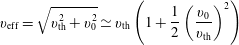 $$\begin{eqnarray}v_{\text{eff}}=\sqrt{v_{\text{th}}^{2}+v_{0}^{2}}\simeq v_{\text{th}}\left(1+\frac{1}{2}\left(\frac{v_{0}}{v_{\text{th}}}\right)^{2}\right)\end{eqnarray}$$
the approximate expression valid in the case in which $v_{0}/v_{\text{th}}\ll 1$
. For the simulations discussed in this paper, in which the velocity distributions are always very close to thermal, this ratio ranges from
$v_{0}/v_{\text{th}}\ll 1$
. For the simulations discussed in this paper, in which the velocity distributions are always very close to thermal, this ratio ranges from $v_{0}/v_{\text{th}}=0.00156$
(highest resolution runs) to
$v_{0}/v_{\text{th}}=0.00156$
(highest resolution runs) to $v_{0}/v_{\text{th}}=0.00795$
(Movie 1 and Movie 2); the effective thermal speed is always very close to the actual thermal speed. However, we do not expect in principle that quantities such as total energy or entropy, when computed using the filtered distribution
$v_{0}/v_{\text{th}}=0.00795$
(Movie 1 and Movie 2); the effective thermal speed is always very close to the actual thermal speed. However, we do not expect in principle that quantities such as total energy or entropy, when computed using the filtered distribution $\bar{f}$
, should be exactly conserved. Figure 2 provides indications of the degree to which these quantities are not conserved in the Case Study simulation discussed below; the results are typical of all of the simulations to be discussed. Both quantities have been normalized by their respective initial values. The simulation continues to
$\bar{f}$
, should be exactly conserved. Figure 2 provides indications of the degree to which these quantities are not conserved in the Case Study simulation discussed below; the results are typical of all of the simulations to be discussed. Both quantities have been normalized by their respective initial values. The simulation continues to $t=10\,000$
but the plots have been truncated in time to show the variations that occur during early times. The asymptotic values that the total energy and entropy take on in the figure remain unchanged, in fact, for the remainder of the simulation.
$t=10\,000$
but the plots have been truncated in time to show the variations that occur during early times. The asymptotic values that the total energy and entropy take on in the figure remain unchanged, in fact, for the remainder of the simulation.

Figure 2. From initial stages of Case Study simulation, evolution of normalized (a) total energy and (b) entropy.
Further details of the transformed simulation scheme can be found in Klimas & Farrell (Reference Klimas and Farrell1994). See appendix B for more information on the simulation set-up used to obtain the results discussed in this paper.
2.2 Initial state
On a spatial interval $(0\leqslant x\leqslant L)$
, Rupp et al. (Reference Rupp, Lopez and Araneda2015) simulated solutions of the unfiltered
$(0\leqslant x\leqslant L)$
, Rupp et al. (Reference Rupp, Lopez and Araneda2015) simulated solutions of the unfiltered $(v_{0}=0)$
system (2.1) with initial state (here, expressed in dimensional form)
$(v_{0}=0)$
system (2.1) with initial state (here, expressed in dimensional form)
 $$\begin{eqnarray}\left.\begin{array}{@{}c@{}}\displaystyle f(x,v,t=0)=f_{0}(v)[1+\unicode[STIX]{x1D700}\cos (k_{m}x)]\\ \displaystyle f_{0}(v)=\frac{1}{v_{\text{th}}\sqrt{2\unicode[STIX]{x03C0}}}\exp \left[-\frac{1}{2}\left(\frac{v}{v_{\text{th}}}\right)^{2}\right],\end{array}\right\}\end{eqnarray}$$
with $L=2\unicode[STIX]{x03C0}/k_{m}$
and
$L=2\unicode[STIX]{x03C0}/k_{m}$
and $ck_{m}/\unicode[STIX]{x1D714}_{pe}=1$
. Using
$ck_{m}/\unicode[STIX]{x1D714}_{pe}=1$
. Using $2L_{k}=L$
and the dimensionless set-up described above, (2.5) can be written
$2L_{k}=L$
and the dimensionless set-up described above, (2.5) can be written
 $$\begin{eqnarray}f(x,v,t=0)=\left(\unicode[STIX]{x03C0}\frac{c}{v_{\text{th}}}\right)\frac{1}{\sqrt{2\unicode[STIX]{x03C0}}}\text{e}^{-(1/2)(\unicode[STIX]{x03C0}(c/v_{\text{th}}))^{2}v^{2}}[1+\unicode[STIX]{x1D700}\cos \unicode[STIX]{x03C0}x].\end{eqnarray}$$
We reproduce the simulations of Rupp et al. (Reference Rupp, Lopez and Araneda2015) by setting $v_{\text{th}}/c=0.4$
, as they did. It should be noted that this choice leads to
$v_{\text{th}}/c=0.4$
, as they did. It should be noted that this choice leads to $\unicode[STIX]{x1D706}_{D}=0.127$
in these dimensionless units. The phase shift introduced by going from
$\unicode[STIX]{x1D706}_{D}=0.127$
in these dimensionless units. The phase shift introduced by going from $(0\leqslant x\leqslant L)$
to
$(0\leqslant x\leqslant L)$
to $(-L_{k}\leqslant x\leqslant L_{k})$
is irrelevant in these periodic solutions. Spatial Fourier modes will be denoted by the index
$(-L_{k}\leqslant x\leqslant L_{k})$
is irrelevant in these periodic solutions. Spatial Fourier modes will be denoted by the index $m$
. In these dimensionless units, the
$m$
. In these dimensionless units, the $m=1$
mode has wavelength
$m=1$
mode has wavelength $2$
; i.e. in dimensional units, the wavelength of the
$2$
; i.e. in dimensional units, the wavelength of the $m=1$
mode is
$m=1$
mode is $2L_{k}=L$
. The neighbourhood of the transition from persisting to arrested Landau damping is explored by varying the value of
$2L_{k}=L$
. The neighbourhood of the transition from persisting to arrested Landau damping is explored by varying the value of $\unicode[STIX]{x1D700}$
.
$\unicode[STIX]{x1D700}$
.
3 Case study
In § 4, we discuss three simulations that span the persisting to arrested critical transition, which we find is at $\unicode[STIX]{x1D700}\simeq 0.0085$
. In this section, we present a detailed discussion of the several phases of a single ‘Case Study’ simulation at
$\unicode[STIX]{x1D700}\simeq 0.0085$
. In this section, we present a detailed discussion of the several phases of a single ‘Case Study’ simulation at $\unicode[STIX]{x1D700}=0.0089$
, just above the transition region.
$\unicode[STIX]{x1D700}=0.0089$
, just above the transition region.
3.1 Overview
Figure 3 shows the time evolution of all field mode magnitudes for this simulation. The modes are ordered in the figure by amplitude. At any particular time, the strongest mode (green) is the $m=1$
mode with wavelength equal to 2
$m=1$
mode with wavelength equal to 2 $(2L_{k})$
. The next mode down (blue) is the
$(2L_{k})$
. The next mode down (blue) is the $m=2$
mode with wavelength 1, and so on. There are four phases of interest in the field evolution: (i) the damping phase, starting very near the beginning of the simulation and lasting until approximately
$m=2$
mode with wavelength 1, and so on. There are four phases of interest in the field evolution: (i) the damping phase, starting very near the beginning of the simulation and lasting until approximately $t=1000$
. (ii) The arrest phase at approximately
$t=1000$
. (ii) The arrest phase at approximately $t=1500$
. (iii) The growth phase from approximately
$t=1500$
. (iii) The growth phase from approximately $t=2000$
to
$t=2000$
to $t=5500$
. (iv) The saturation phase, starting at approximately
$t=5500$
. (iv) The saturation phase, starting at approximately $t=6000$
.
$t=6000$
.

Figure 3. Evolution in time of all field mode magnitudes in the Case Study $(\unicode[STIX]{x1D700}=0.0089)$
simulation.
$(\unicode[STIX]{x1D700}=0.0089)$
simulation.
Figure 4 shows the electric field at approximately $t=3000$
, during the growth phase, and at approximately
$t=3000$
, during the growth phase, and at approximately $t=6200$
, during the saturation phase. At the earlier time the
$t=6200$
, during the saturation phase. At the earlier time the $m=1$
mode is strongly dominant and, thus, the field is a simple sine wave. An excellent fit to the field evolution at this earlier time is given by
$m=1$
mode is strongly dominant and, thus, the field is a simple sine wave. An excellent fit to the field evolution at this earlier time is given by
 $$\begin{eqnarray}E(t)=E_{0}\text{e}^{\unicode[STIX]{x1D6FE}t}\sin \unicode[STIX]{x03C0}x\cos \unicode[STIX]{x1D6FA}t=E_{0}\text{e}^{\unicode[STIX]{x1D6FE}t}[\text{sin}\,\unicode[STIX]{x03C0}(x-v_{\text{res}}t)+\sin \unicode[STIX]{x03C0}(x+v_{\text{res}}t)],\end{eqnarray}$$
with $\log _{10}E_{0}=-7.61084$
,
$\log _{10}E_{0}=-7.61084$
, $\unicode[STIX]{x1D6FA}=1.2722$
in units of
$\unicode[STIX]{x1D6FA}=1.2722$
in units of $\unicode[STIX]{x1D714}_{pe}$
,
$\unicode[STIX]{x1D714}_{pe}$
, $\unicode[STIX]{x1D6FE}=0.0005$
and with the resonant speed
$\unicode[STIX]{x1D6FE}=0.0005$
and with the resonant speed $v_{\text{res}}=\unicode[STIX]{x1D6FA}/\unicode[STIX]{x03C0}=0.4050$
being the speed at which electrons must move to traverse the
$v_{\text{res}}=\unicode[STIX]{x1D6FA}/\unicode[STIX]{x03C0}=0.4050$
being the speed at which electrons must move to traverse the $m=1$
mode wavelength in one of its oscillation periods. Similar fits are available for the three transition study simulations that will be discussed in § 4, each with its own value for
$m=1$
mode wavelength in one of its oscillation periods. Similar fits are available for the three transition study simulations that will be discussed in § 4, each with its own value for $\unicode[STIX]{x1D6FE}$
.
$\unicode[STIX]{x1D6FE}$
.

Figure 4. Electric field at approximately $t=3000$
(red, left ordinate) during growth phase and at approximately
$t=3000$
(red, left ordinate) during growth phase and at approximately $t=6200$
(blue, right ordinate) during saturation phase from Case Study
$t=6200$
(blue, right ordinate) during saturation phase from Case Study $(\unicode[STIX]{x1D700}=0.0089)$
simulation.
$(\unicode[STIX]{x1D700}=0.0089)$
simulation.
For the purpose of understanding whether or not evidence of trapping is found in any of these simulations, it is important to note that we find the total electric field never propagates spatially, it simply oscillates temporally, as shown by the first term in (3.1). This is true for all simulations discussed in this paper, including the saturation phase of the Case Study ( $\unicode[STIX]{x1D700}=0.0089$
) under discussion in this section in which the simple sinusoidal shape can be somewhat distorted, as shown in figure 4, but the wave still does not propagate spatially. Nevertheless, as shown by the second term in (3.1) the total field can be written as the sum of two modes propagating at
$\unicode[STIX]{x1D700}=0.0089$
) under discussion in this section in which the simple sinusoidal shape can be somewhat distorted, as shown in figure 4, but the wave still does not propagate spatially. Nevertheless, as shown by the second term in (3.1) the total field can be written as the sum of two modes propagating at $\pm v_{\text{res}}$
. This form, with
$\pm v_{\text{res}}$
. This form, with $\unicode[STIX]{x1D6FE}=0$
, is in agreement with the two-wave asymptotic field example discussed by Lancellotti & Dorning (Reference Lancellotti and Dorning1998a
). One of the Transition Study simulations discussed in § 4 exhibits
$\unicode[STIX]{x1D6FE}=0$
, is in agreement with the two-wave asymptotic field example discussed by Lancellotti & Dorning (Reference Lancellotti and Dorning1998a
). One of the Transition Study simulations discussed in § 4 exhibits $\unicode[STIX]{x1D6FE}\simeq 0$
for large times and, thus, is a good example of the two-wave example of Lancellotti and Dorning.
$\unicode[STIX]{x1D6FE}\simeq 0$
for large times and, thus, is a good example of the two-wave example of Lancellotti and Dorning.
3.2 Phase-space distribution
Figures 5 and 6 provide alternate views of the $\unicode[STIX]{x1D700}=0.0089$
electron phase-space distribution at
$\unicode[STIX]{x1D700}=0.0089$
electron phase-space distribution at $t=3000$
with, in both figures, the space-averaged distribution removed. A very small filter width
$t=3000$
with, in both figures, the space-averaged distribution removed. A very small filter width $v_{0}=0.000637$
has been used to obtain this result. Figure 5 can be compared to figure 1(a), which was taken from the same simulation with the same filter width at a much earlier time. It can be seen that at the later time of figure 5 the filamentation velocity scale has evolved downward to below the filter width and the wave structure perturbing the space-averaged distribution has been revealed.
$v_{0}=0.000637$
has been used to obtain this result. Figure 5 can be compared to figure 1(a), which was taken from the same simulation with the same filter width at a much earlier time. It can be seen that at the later time of figure 5 the filamentation velocity scale has evolved downward to below the filter width and the wave structure perturbing the space-averaged distribution has been revealed.

Figure 5. Phase-space distribution with space-averaged distribution removed at $t=3000$
with
$t=3000$
with $v_{o}=0.000637$
.
$v_{o}=0.000637$
.

Figure 6. Phase-space distribution with space-averaged distribution removed at $t=3000$
with
$t=3000$
with $v_{o}=0.000637$
.
$v_{o}=0.000637$
.
The waveforms shown in figures 5 and 6 and figure 1(b) are actually the same waveform seen first in the damping phase of the simulation and later in the growth phase. It consists of narrow structures at the resonant velocities $v_{\text{res}}=\pm (\unicode[STIX]{x1D6FA}/\unicode[STIX]{x03C0})$
, in which
$v_{\text{res}}=\pm (\unicode[STIX]{x1D6FA}/\unicode[STIX]{x03C0})$
, in which $\unicode[STIX]{x1D6FA}$
is the oscillation frequency of the electric field, plus weaker waves between the resonant velocities. These weaker waves appear more prominent in figure 1 because they are shown relative to the peaked resonance waves, which have been smoothed and lowered by the broad filter used to obtain those early time results. Further, the weaker interior waves are coupled to the waves at the resonant velocities, which are propagating at the resonant velocities in opposite directions. Thus, the stretched out appearance of the interior waves in figure 5 arises at one time while the non-stretched-out appearance in figure 1 arises at another.
$\unicode[STIX]{x1D6FA}$
is the oscillation frequency of the electric field, plus weaker waves between the resonant velocities. These weaker waves appear more prominent in figure 1 because they are shown relative to the peaked resonance waves, which have been smoothed and lowered by the broad filter used to obtain those early time results. Further, the weaker interior waves are coupled to the waves at the resonant velocities, which are propagating at the resonant velocities in opposite directions. Thus, the stretched out appearance of the interior waves in figure 5 arises at one time while the non-stretched-out appearance in figure 1 arises at another.
In the following § 3.3, the structure of the narrow resonance waves at the resonant velocities will be examined in detail with emphasis on three selected times, $t=700$
during the damping phase,
$t=700$
during the damping phase, $t=1500$
at the arrest time and
$t=1500$
at the arrest time and $t=3000$
during the growth phase. Supplementary Movies 3, 4 and 5 are available at https://doi.org/10.1017/S002237781700054X and show the evolution in time of the global phase-space distributions minus space-averaged component, as shown in figures 5 and 6, at these selected times. An important conclusion that can be reached by comparing these movies is that there appears to be no discernible difference in the waveforms associated with the different phases of the simulation. In the following section we show that there are, in fact, significant differences but they lie within the narrow resonance wave structures and are not discernible in the global images. The waveforms shown in these movies pervade all phases of all of the simulations discussed in this paper except for the saturation phase of this Case Study simulation.
$t=3000$
during the growth phase. Supplementary Movies 3, 4 and 5 are available at https://doi.org/10.1017/S002237781700054X and show the evolution in time of the global phase-space distributions minus space-averaged component, as shown in figures 5 and 6, at these selected times. An important conclusion that can be reached by comparing these movies is that there appears to be no discernible difference in the waveforms associated with the different phases of the simulation. In the following section we show that there are, in fact, significant differences but they lie within the narrow resonance wave structures and are not discernible in the global images. The waveforms shown in these movies pervade all phases of all of the simulations discussed in this paper except for the saturation phase of this Case Study simulation.
3.3 Resonance wave structure
Figure 7 shows the details, at the high velocity resolution of figure 5, of one of the resonance wave structures, in this case at the negative velocity resonance $(v_{\text{res}}=-0.405)$
. We have observed this structure, with small but important variations that are discussed below, throughout all phases of this
$(v_{\text{res}}=-0.405)$
. We have observed this structure, with small but important variations that are discussed below, throughout all phases of this $\unicode[STIX]{x1D700}=0.0098$
simulation except the saturation phase, as well as throughout the simulations spanning the transition from damping to growth to be discussed below in § 4. At any fixed velocity, the structure amounts to a simple
$\unicode[STIX]{x1D700}=0.0098$
simulation except the saturation phase, as well as throughout the simulations spanning the transition from damping to growth to be discussed below in § 4. At any fixed velocity, the structure amounts to a simple $m=1$
wave. Crossing the resonant velocity generally leads to a sharp reversal in sign. The several components of the structure propagate together and remain in fixed relative positions. This structure is ubiquitous in these simulations.
$m=1$
wave. Crossing the resonant velocity generally leads to a sharp reversal in sign. The several components of the structure propagate together and remain in fixed relative positions. This structure is ubiquitous in these simulations.

Figure 7. Detail from figure 5 showing the negative velocity resonant wave structure perturbing the space-averaged phase-space distribution.
Figure 8 shows the resonance wave structure in somewhat lower velocity resolution $(v_{0}=0.00318)$
at three times; (a) at approximately
$(v_{0}=0.00318)$
at three times; (a) at approximately $t=700$
during the damping phase, (b) at arrest at approximately
$t=700$
during the damping phase, (b) at arrest at approximately $t=1500$
and (c) during the growth phase at approximately
$t=1500$
and (c) during the growth phase at approximately $t=3000$
. In each case, the time has been adjusted slightly to reach a maximum in the electric field strength at the oscillation phase shown in red in figure 4; i.e. with the force on the electrons due to the field outward from
$t=3000$
. In each case, the time has been adjusted slightly to reach a maximum in the electric field strength at the oscillation phase shown in red in figure 4; i.e. with the force on the electrons due to the field outward from $x=0$
, to the left on the left and to the right on the right. The forces peak at
$x=0$
, to the left on the left and to the right on the right. The forces peak at $x=\pm 0.5$
while the particle concentrations at
$x=\pm 0.5$
while the particle concentrations at $x=0$
and
$x=0$
and $x=\pm 1$
are at the minima in this force field. In each case, these patterns propagate from right to left at the relevant resonance speed while they persist over multiple oscillation periods in the electric field.
$x=\pm 1$
are at the minima in this force field. In each case, these patterns propagate from right to left at the relevant resonance speed while they persist over multiple oscillation periods in the electric field.

Figure 8. Resonant wave structure from the $\unicode[STIX]{x1D700}=0.0098$
simulation at three times. (a) Damping phase,
$\unicode[STIX]{x1D700}=0.0098$
simulation at three times. (a) Damping phase, $t=700$
. (b) At reversal,
$t=700$
. (b) At reversal, $t=1500$
. (c) Growth phase
$t=1500$
. (c) Growth phase $t=3000$
.
$t=3000$
.
In figure 8(a), we note the presence of a positive perturbation bridging the gap between the larger positive island in the centre of the figure at lower speed and the partially visible positive island at higher speed at the left side of the figure. This perturbation represents a stream of electrons at the position of an electric field strength maximum at this time; these electrons are being accelerated out of the lower speed island and into the higher speed island during the Landau damping phase. Similarly, in panel (c) we note the presence of a positive perturbation bridging the gap between the positive island at the right edge of the figure at higher speed and the central positive island at lower speed. (Figure 7 provides a higher resolution view of this perturbation at a different phase in the electric field oscillation.) This electron stream also lies at the position of an electric field strength maximum at this time; the electrons are being decelerated out of the higher speed island and into the lower speed island during the Landau growth phase. Notably, panel (b), obtained during the arrest phase when the transfer of energy between electrons and field has paused, contains no evidence of the electron streams seen in (a,b). We interpret these streams as evidence of the expected (Dawson Reference Dawson1961) transfers of energy between electrons and electric field during Landau damping or growth. During the Landau damping phase the electrons gain energy at the expense of the field and during the Landau growth phase the electrons lose energy to the field.
We emphasize that the patterns exhibited in figure 8 persist and propagate at the resonant velocity essentially unchanged over many electric field oscillation periods and, thus, through many $m=1$
wavelengths. There is no evidence of trapping during the damping, arrest, or growth phases in this simulation for the case of
$m=1$
wavelengths. There is no evidence of trapping during the damping, arrest, or growth phases in this simulation for the case of $\unicode[STIX]{x1D700}$
just above its transition value.
$\unicode[STIX]{x1D700}$
just above its transition value.
3.4 Saturation phase
As this simulation passes through the saturation phase, the resonance wave on the space-averaged phase-space distribution alters considerably for the first time. Figure 9 shows this alteration during a time interval covering just the first peak in electric field strength shown in figure 3; i.e. from $t=5000$
to
$t=5000$
to $6700$
. By fitting the total electric field evolution through the growth phase, we have determined that its oscillation frequency
$6700$
. By fitting the total electric field evolution through the growth phase, we have determined that its oscillation frequency $\unicode[STIX]{x1D6FA}=1.2722$
, leading to the resonant speed
$\unicode[STIX]{x1D6FA}=1.2722$
, leading to the resonant speed $v_{\text{res}}=0.405$
. Figure 9 shows the results seen by an observer moving with the negative resonant velocity so that at the several times shown the position of the wave structure appears relatively stationary.
$v_{\text{res}}=0.405$
. Figure 9 shows the results seen by an observer moving with the negative resonant velocity so that at the several times shown the position of the wave structure appears relatively stationary.

Figure 9. Resonance wave structure on the space-averaged phase-space distribution at negative velocity in the simulation saturation phase. (a) $t=5000$
. (b)
$t=5000$
. (b) $t=6200$
. (c)
$t=6200$
. (c) $t=6500$
. (d)
$t=6500$
. (d) $t=6700$
.
$t=6700$
.

Figure 10. Electric field mode magnitudes for (a) super-transition $(\unicode[STIX]{x1D700}=0.0086)$
, (b) transition
$(\unicode[STIX]{x1D700}=0.0086)$
, (b) transition $(\unicode[STIX]{x1D700}=0.0085)$
and (c) sub-transition
$(\unicode[STIX]{x1D700}=0.0085)$
and (c) sub-transition $(\unicode[STIX]{x1D700}=0.0084)$
simulations.
$(\unicode[STIX]{x1D700}=0.0084)$
simulations.
Panel (a), at $t=5000$
, shows the resonance wave as the simulation approaches the saturation phase. The wave structure shown in this panel can be compared to that shown in figure 7 at
$t=5000$
, shows the resonance wave as the simulation approaches the saturation phase. The wave structure shown in this panel can be compared to that shown in figure 7 at $t=3000$
to see that, as the saturation phase is approached, the electron stream from high to low speed is weakened; the transfer of energy from particles to field weakens as the saturation phase is approached. At
$t=3000$
to see that, as the saturation phase is approached, the electron stream from high to low speed is weakened; the transfer of energy from particles to field weakens as the saturation phase is approached. At $t=6200$
in panel (b), the stream has vanished and the electrons represented by the positive excess at approximately
$t=6200$
in panel (b), the stream has vanished and the electrons represented by the positive excess at approximately $x=0.1$
have bunched together. The magnitude of this positive excess has strengthened considerably, producing a relatively strong local density perturbation, leading with a positive contribution and trailing with a negative contribution. Shortly thereafter, at
$x=0.1$
have bunched together. The magnitude of this positive excess has strengthened considerably, producing a relatively strong local density perturbation, leading with a positive contribution and trailing with a negative contribution. Shortly thereafter, at $t=6500$
in panel (c), the local positive density perturbation has moved to a lower speed and is falling behind the higher speed negative perturbation. At this time, a new negative perturbation at the lower speed has formed. Finally, at
$t=6500$
in panel (c), the local positive density perturbation has moved to a lower speed and is falling behind the higher speed negative perturbation. At this time, a new negative perturbation at the lower speed has formed. Finally, at $t=6700$
in panel (d), the positive density perturbation has rotated about the negative perturbation and is about to join the positive region in back of it. This sequence occurs during the first peak in the electric field strength shown in figure 3. A similar but less well defined sequence takes place during the second field strength peak shown in that figure. Although not shown, this simulation has been extended to
$t=6700$
in panel (d), the positive density perturbation has rotated about the negative perturbation and is about to join the positive region in back of it. This sequence occurs during the first peak in the electric field strength shown in figure 3. A similar but less well defined sequence takes place during the second field strength peak shown in that figure. Although not shown, this simulation has been extended to $t=20\,000$
. We find the field strength fluctuating as in the saturation phase shown in figure 3 with no evident long-term trend.
$t=20\,000$
. We find the field strength fluctuating as in the saturation phase shown in figure 3 with no evident long-term trend.
While the rotation of positive excess about the negative perturbation region shown in figure 9 may give the impression of a trapping phenomenon, this is clearly not the correct interpretation. Approximately 340 electric field oscillation periods have elapsed during the sequence shown in the figure and, simultaneously, the waveform shown has propagated that number of $m=1$
wavelengths in the field; i.e. that number of simulation ‘boxes’. The perturbation waveform does not represent electrons trapped in an electric field potential. In addition, we note that the stability of the perturbation’s position in the panels of figure 9 is a strong confirmation of its
$m=1$
wavelengths in the field; i.e. that number of simulation ‘boxes’. The perturbation waveform does not represent electrons trapped in an electric field potential. In addition, we note that the stability of the perturbation’s position in the panels of figure 9 is a strong confirmation of its $v_{\text{res}}=\unicode[STIX]{x1D6FA}/\unicode[STIX]{x03C0}$
propagation speed.
$v_{\text{res}}=\unicode[STIX]{x1D6FA}/\unicode[STIX]{x03C0}$
propagation speed.
4 Transition study
In this section we focus on the properties of the waveform superposed on the space-averaged electron phase-space distribution as $\unicode[STIX]{x1D700}$
is varied from below to above its transition value. Three simulations are studied, corresponding to
$\unicode[STIX]{x1D700}$
is varied from below to above its transition value. Three simulations are studied, corresponding to $\unicode[STIX]{x1D700}=0.0084$
,
$\unicode[STIX]{x1D700}=0.0084$
, $0.0085$
and
$0.0085$
and $0.0086$
. For ease of discussion, we will call these the ‘Sub-Transition’, ‘Transition’ and ‘Super-Transition’ simulations, respectively.
$0.0086$
. For ease of discussion, we will call these the ‘Sub-Transition’, ‘Transition’ and ‘Super-Transition’ simulations, respectively.
4.1 Field magnitudes
Figure 10 shows the evolution with time of the electric field mode magnitudes for these three cases. Panel (a) shows for the Super-Transition simulation the familiar initial damping phase, the arrest phase, and then the growth phase, which continues at the end of the simulation. The Transition simulation, shown in panel (b), continues on with essentially no consequent growth or decay following the initial damping phase. The Sub-Transition simulation, shown in panel (c), exhibits a shift from the initial faster damping to the later slower damping, which continues at the end of the simulation. An extension of this simulation (not shown) to $t=20\,000$
shows continuing unchanged damping and an additional simulation (not shown) with
$t=20\,000$
shows continuing unchanged damping and an additional simulation (not shown) with $\unicode[STIX]{x1D700}=0.0042$
shows the expected faster damping down to the digital noise level at approximately
$\unicode[STIX]{x1D700}=0.0042$
shows the expected faster damping down to the digital noise level at approximately $10^{-18}$
with no further evolution after that. No evidence for other than persisting damping has been found in any sub-transition simulation.
$10^{-18}$
with no further evolution after that. No evidence for other than persisting damping has been found in any sub-transition simulation.
During the initial damping phase, all three simulations exhibit perturbations to their space-averaged phase-space distributions that are similar to that shown in figure 1(b). Because the $m=1$
electric field mode is very dominant in all three simulations, they all exhibit a simple sinusoidal electric field as shown in figure 4 for all times. For all three cases, the field does not propagate spatially but does oscillate sinusoidally with time. Figures 5 and 6 are representative of the global waveform found on the space-averaged phase-space distribution in all three simulations. It appears that this single waveform can be found superposed on the space-averaged phase-space distribution of any of the simulations discussed in this paper at any time except during the saturation phase, when it exists.
$m=1$
electric field mode is very dominant in all three simulations, they all exhibit a simple sinusoidal electric field as shown in figure 4 for all times. For all three cases, the field does not propagate spatially but does oscillate sinusoidally with time. Figures 5 and 6 are representative of the global waveform found on the space-averaged phase-space distribution in all three simulations. It appears that this single waveform can be found superposed on the space-averaged phase-space distribution of any of the simulations discussed in this paper at any time except during the saturation phase, when it exists.
4.2 Resonance wave structure
Figure 11 shows the negative velocity resonance waveforms superposed on the space-averaged phase-space distributions for the Super-Transition (a), Transition (b) and Sub-Transition (c) simulations at times very near the ends of the simulations at $t=10\,000$
. For such large times, it is possible to use a very narrow filamentation filter width
$t=10\,000$
. For such large times, it is possible to use a very narrow filamentation filter width $v_{0}=0.000637$
to obtain high velocity resolution. Even so, it is possible that the waveforms shown in the figure are not fully resolved.
$v_{0}=0.000637$
to obtain high velocity resolution. Even so, it is possible that the waveforms shown in the figure are not fully resolved.

Figure 11. Negative velocity resonance waveforms superposed on the space-averaged phase-space distributions of the (a) super-transition $(\unicode[STIX]{x1D700}=0.0086)$
, (b) transition
$(\unicode[STIX]{x1D700}=0.0086)$
, (b) transition $(\unicode[STIX]{x1D700}=0.0085)$
and (c) sub-transition
$(\unicode[STIX]{x1D700}=0.0085)$
and (c) sub-transition $(\unicode[STIX]{x1D700}=0.0084)$
simulations.
$(\unicode[STIX]{x1D700}=0.0084)$
simulations.
Figure 11(a) is from the Super-Transition simulation growth phase, which continues to the end of the simulation. The figure reveals an electron stream from high to low speed that, as discussed above, we suggest is a signature of the transfer of energy from the electrons to the electric field during this growth phase. Panel (c) is from the Sub-Transition simulation late damping phase near the end of the simulation. This figure reveals a stream from low to high speed that we suggest is a signature of the transfer of energy from the electric field to the electrons during this damping phase. Consistent with this interpretation, panel (b) from the Transition simulation shows no stream and, thus, no energy transfer while the electric field magnitude remains essentially stationary (see figure 10 b).
The similarity of the perturbation waveforms shown in figure 11 from the three Transition Study simulations to those shown in figure 8 (albeit at lower velocity resolution and with the order from top to bottom reversed) from the damping, arrest and growth phases of the Case Study simulation is striking. Each of the waveforms found in the individual Transition Study simulations can be found in the phases of the Case Study simulation. The waveforms of the Transition Study simulations are not unique to the individual simulations of that study.
5 Conclusions
We have discussed a filtered Vlasov–Poisson simulation study of the transition from persisting to arrested Landau damping that is produced by varying the parameter $\unicode[STIX]{x1D700}$
in the initial state (2.6). The objective of the study was to find evidence of a second-order phase transition in the electron phase-space distribution at the
$\unicode[STIX]{x1D700}$
in the initial state (2.6). The objective of the study was to find evidence of a second-order phase transition in the electron phase-space distribution at the $\unicode[STIX]{x1D700}$
transition value to complement the well-established evidence of such a phase transition found earlier in the electric field evolution (Ivanov et al.
Reference Ivanov, Cairns and Robinson2004; Ivanov, Vladimirov & Robinson Reference Ivanov, Vladimirov and Robinson2005; Rupp et al.
Reference Rupp, Lopez and Araneda2015). To that end, a single Case Study simulation with
$\unicode[STIX]{x1D700}$
transition value to complement the well-established evidence of such a phase transition found earlier in the electric field evolution (Ivanov et al.
Reference Ivanov, Cairns and Robinson2004; Ivanov, Vladimirov & Robinson Reference Ivanov, Vladimirov and Robinson2005; Rupp et al.
Reference Rupp, Lopez and Araneda2015). To that end, a single Case Study simulation with $\unicode[STIX]{x1D700}$
somewhat above the transition neighbourhood has been carried out to provide a reference point to help our further examination of three additional transition simulations that have been run with
$\unicode[STIX]{x1D700}$
somewhat above the transition neighbourhood has been carried out to provide a reference point to help our further examination of three additional transition simulations that have been run with $\unicode[STIX]{x1D700}$
bracketing and near to the transition value. The Case Study simulation exhibited four phases in its evolution, an initial damping phase, an arrest phase during which the electric field strength remained approximately constant for a large number of oscillation periods, then a growth phase and finally a saturation phase. The transition simulations also exhibited the initial damping phase but then evolved into either growth (Super-Transition simulation), approximate stationarity (Transition simulation) or damping (Sub-Transition simulation), where they all remained. An important feature of our study is our comparison of the final states of the transition simulations to the relevant phases of the Case Study simulation.
$\unicode[STIX]{x1D700}$
bracketing and near to the transition value. The Case Study simulation exhibited four phases in its evolution, an initial damping phase, an arrest phase during which the electric field strength remained approximately constant for a large number of oscillation periods, then a growth phase and finally a saturation phase. The transition simulations also exhibited the initial damping phase but then evolved into either growth (Super-Transition simulation), approximate stationarity (Transition simulation) or damping (Sub-Transition simulation), where they all remained. An important feature of our study is our comparison of the final states of the transition simulations to the relevant phases of the Case Study simulation.
Our use of the filtered Vlasov–Poisson system (2.1) allowed us to examine the phase-space probability distribution in a novel manner. Since the filamentation evolves to finer velocity scales as time increases, filters of different widths become effective in removing the filamentation at different times. We took advantage of this behaviour by running each simulation several times using different filter widths. Runs using a wide filter removed the filamentation earlier but revealed a velocity-broadened result, runs with a narrower filter removed the filamentation later with better velocity resolution, and runs with a very narrow filter removed the filamentation much later with excellent velocity resolution. In this way, we have found a universal underlying waveform that is normally hidden under the dominant filamentation; it perturbs the space-averaged phase-space distribution during all but the saturation phase, arising as early as $t=10$
(see Movie 2) during the Landau damping phase. This waveform is dominated by very narrow structures straddling the resonant velocities where the electrons traverse the dominant electric field wavelength in exactly its oscillation period. Using our higher resolution simulation results, we have been able to resolve these structures to provide images of the expected transfer of energy between electrons and electric field during the damping and growth phases and have shown that no such transfer occurs during an arrest or stationary phase.
$t=10$
(see Movie 2) during the Landau damping phase. This waveform is dominated by very narrow structures straddling the resonant velocities where the electrons traverse the dominant electric field wavelength in exactly its oscillation period. Using our higher resolution simulation results, we have been able to resolve these structures to provide images of the expected transfer of energy between electrons and electric field during the damping and growth phases and have shown that no such transfer occurs during an arrest or stationary phase.
A central point of this paper is that we see the ubiquitous phase-space waveform at almost any time in any of our simulations. We do have reasons for confidence in this result. The first is that the filtered code has been applied successfully many times to the standard tests of 1-D electrostatic Vlasov–Poisson codes that are in the literature (Klimas Reference Klimas1987; Klimas & Farrell Reference Klimas and Farrell1994) and it has also been applied successfully to explain space plasma physics observations (Klimas Reference Klimas1983b
; Fitzenreiter, Klimas & Scudder Reference Fitzenreiter, Klimas and Scudder1984; Klimas & Fitzenreiter Reference Klimas and Fitzenreiter1988; Fitzenreiter, Scudder & Klimas Reference Fitzenreiter, Scudder and Klimas1990; Klimas Reference Klimas1990; Fitzenreiter et al.
Reference Fitzenreiter, Vinas, Klimas, Lepping, Kaiser and Onsager1996). Further, the filtered simulations behave exactly as expected theoretically, with the field independent of $v_{0}$
and with the evolution of the phase-space distribution unchanged by the choice of
$v_{0}$
and with the evolution of the phase-space distribution unchanged by the choice of $v_{0}$
except for its velocity resolution. However, we cannot prove that our results are not a product of the particular filter function (2.3) that we have used; although other filters have been proposed (Klimas Reference Klimas1987), we have used only one. An independent study might confirm the appearance of the ubiquitous phase-space waveform but it is difficult to propose an alternate collisionless Vlasov–Poisson simulation technique that might succeed. While Pezzi et al. (Reference Pezzi, Camporeale and Valentini2016) were able to show that the approach due to Black et al. (Reference Black, Germaschewski, Bhattacharjee and Ng2013) is not viable for removing filamentation and, then recurrence, from the long-time evolution of linear Landau damping solutions, the work of Black et al. may still be of particular relevance here. One must wonder, what is the relationship of the phase-space waveform that we have found pervading almost all phases of our collisionless Landau damping simulations to the most slowly damped weakly collisional eigenmode that Black et al. have found emerges later in their linear Landau damping simulation? A comparison of figure 4 of Black et al. to figure 5 of this paper suggests a close relationship. The theoretical analyses of Ng et al. (Reference Ng, Bhattacharjee and Skiff1999, Reference Ng, Bhattacharjee and Skiff2004) suggests that there should be a close relationship. With further study, can the apparent close relationship between our ubiquitous waveform and the eigenmode shown by Black et al. in their figure 4 be developed into the independent study that we lack?
$v_{0}$
except for its velocity resolution. However, we cannot prove that our results are not a product of the particular filter function (2.3) that we have used; although other filters have been proposed (Klimas Reference Klimas1987), we have used only one. An independent study might confirm the appearance of the ubiquitous phase-space waveform but it is difficult to propose an alternate collisionless Vlasov–Poisson simulation technique that might succeed. While Pezzi et al. (Reference Pezzi, Camporeale and Valentini2016) were able to show that the approach due to Black et al. (Reference Black, Germaschewski, Bhattacharjee and Ng2013) is not viable for removing filamentation and, then recurrence, from the long-time evolution of linear Landau damping solutions, the work of Black et al. may still be of particular relevance here. One must wonder, what is the relationship of the phase-space waveform that we have found pervading almost all phases of our collisionless Landau damping simulations to the most slowly damped weakly collisional eigenmode that Black et al. have found emerges later in their linear Landau damping simulation? A comparison of figure 4 of Black et al. to figure 5 of this paper suggests a close relationship. The theoretical analyses of Ng et al. (Reference Ng, Bhattacharjee and Skiff1999, Reference Ng, Bhattacharjee and Skiff2004) suggests that there should be a close relationship. With further study, can the apparent close relationship between our ubiquitous waveform and the eigenmode shown by Black et al. in their figure 4 be developed into the independent study that we lack?
In the absence of the Case Study simulation, we might have argued that the change in structure of the peaked resonance waves from one exhibiting energy flow from field to electrons during the sub-transition simulation, to one showing no energy flow during the transition simulation, and finally to one showing energy flow from electrons to field during the super-transition simulation could represent a phase transition in the electron phase-space distribution. However, each of these forms of the peaked resonance waves occur in the single Case Study simulation during its damping, arrest or growth phases. We cannot argue that these structural changes are due solely to changes in $\unicode[STIX]{x1D700}$
in the transition simulations when we find the same changes in a single simulation at one
$\unicode[STIX]{x1D700}$
in the transition simulations when we find the same changes in a single simulation at one $\unicode[STIX]{x1D700}$
value. Accordingly, we conclude from our simulation study that there is no evidence in the electron phase-space distribution in support of a second-order phase transition in the plasma even though the evidence for the transition is strong in the electric field evolution. We have no explanation for this apparent contradiction at present.
$\unicode[STIX]{x1D700}$
value. Accordingly, we conclude from our simulation study that there is no evidence in the electron phase-space distribution in support of a second-order phase transition in the plasma even though the evidence for the transition is strong in the electric field evolution. We have no explanation for this apparent contradiction at present.
We have found that the saturation phase in the Case Study simulation is the only time in all of our simulations during which the underlying universal waveform is altered significantly. A trapping-like sequence occurs in which the phase-space density of the resonance structure is bunched, the bunched density peak rotates about a density minimum residing at the resonant velocity, and then it joins the higher density region just in back of the minimum. However, this sequence extends over hundreds of electric field oscillation periods while the modified resonance structure traverses the same number of wavelengths in the dominant electric field mode. This is a resonance process that does not involve trapping. In fact, we have found no evidence for trapping at any stage of any of the simulations under discussion here. It is interesting that the O’Neil trapping time (O’Neil Reference O’Neil1965) for the Case Study simulation is $t_{\text{trap}}=66.6$
and for the Super Transition simulation is
$t_{\text{trap}}=66.6$
and for the Super Transition simulation is $t_{\text{trap}}=68.1$
, both of which are far earlier than the arrest times for those simulations, which are at approximately
$t_{\text{trap}}=68.1$
, both of which are far earlier than the arrest times for those simulations, which are at approximately $t=1500$
and
$t=1500$
and $t=3500$
respectively. We note that Ivanov & Cairns (Reference Ivanov and Cairns2006), in their discussion of a simulation near but clearly above the transition (threshold) perturbation amplitude, have argued that trapping does not play a role in either the establishment of the arrest phase or of the saturation phase. However, they also report that saturation, in their simulation, is due to the generation of phase-space turbulence. No evidence of turbulence has been found at any stage of our simulations.
$t=3500$
respectively. We note that Ivanov & Cairns (Reference Ivanov and Cairns2006), in their discussion of a simulation near but clearly above the transition (threshold) perturbation amplitude, have argued that trapping does not play a role in either the establishment of the arrest phase or of the saturation phase. However, they also report that saturation, in their simulation, is due to the generation of phase-space turbulence. No evidence of turbulence has been found at any stage of our simulations.
From the results shown in the panels of figure 10, we can conclude that the transition value for the perturbation strength is $\unicode[STIX]{x1D700}^{\ast }\simeq 0.0085$
. At that value, the field evolution shown in figure 10(b) is compatible with the two-wave case of Lancellotti & Dorning (Reference Lancellotti and Dorning1998a
). As discussed in § 3.1, the field evolution can be expressed as the sum of two sin waves propagating at the opposing resonant velocities. Further, for as far as our simulation goes, the almost constant amplitude of the dominant field mode is consistent with the constant non-zero asymptotic field strength predicted by Lancellotti and Dorning. We note that our estimate for
$\unicode[STIX]{x1D700}^{\ast }\simeq 0.0085$
. At that value, the field evolution shown in figure 10(b) is compatible with the two-wave case of Lancellotti & Dorning (Reference Lancellotti and Dorning1998a
). As discussed in § 3.1, the field evolution can be expressed as the sum of two sin waves propagating at the opposing resonant velocities. Further, for as far as our simulation goes, the almost constant amplitude of the dominant field mode is consistent with the constant non-zero asymptotic field strength predicted by Lancellotti and Dorning. We note that our estimate for $\unicode[STIX]{x1D700}^{\ast }$
is quite consistent with the value
$\unicode[STIX]{x1D700}^{\ast }$
is quite consistent with the value $\unicode[STIX]{x1D700}^{\ast }=0.00845$
found by Ivanov et al. (Reference Ivanov, Cairns and Robinson2004). However, right at that initial perturbation strength their simulation showed the field strength decaying algebraically, in contradiction to Lancellotti and Dorning. We have not been able to reproduce that result.
$\unicode[STIX]{x1D700}^{\ast }=0.00845$
found by Ivanov et al. (Reference Ivanov, Cairns and Robinson2004). However, right at that initial perturbation strength their simulation showed the field strength decaying algebraically, in contradiction to Lancellotti and Dorning. We have not been able to reproduce that result.
A final caution: as noted in § 2.2, the Debye length for all of our simulations is $\unicode[STIX]{x1D706}_{D}=0.127$
, measured in the dimensionless units defined in that section. The panels of figure 9, exhibiting features of the negative velocity resonance wave during the saturation phase of the Case Study simulation, show spatial structures that are somewhat larger but still comparable in size to this length. In this situation, might unshielded two-particle correlations produce significant contributions to the right-hand side of the Vlasov equation (Krall & Trivelpiece Reference Krall, Trivelpiece and Harnwell1986) in these spatial structures? For the parameter set that has been used in this study (§ 2.2), is the evolution into the saturation phase actually a passage into a regime in which the Vlasov approximation is no longer valid? At present, we are attempting to answer these difficult questions. If we are successful, we will report our results in the future.
$\unicode[STIX]{x1D706}_{D}=0.127$
, measured in the dimensionless units defined in that section. The panels of figure 9, exhibiting features of the negative velocity resonance wave during the saturation phase of the Case Study simulation, show spatial structures that are somewhat larger but still comparable in size to this length. In this situation, might unshielded two-particle correlations produce significant contributions to the right-hand side of the Vlasov equation (Krall & Trivelpiece Reference Krall, Trivelpiece and Harnwell1986) in these spatial structures? For the parameter set that has been used in this study (§ 2.2), is the evolution into the saturation phase actually a passage into a regime in which the Vlasov approximation is no longer valid? At present, we are attempting to answer these difficult questions. If we are successful, we will report our results in the future.
Acknowledgements
Helpful discussions with V. M. Uritsky are gratefully acknowledged. A.F.V. and A.J.K. would like to thank the NASA/Wind-SWE project for their support. J.A.A. would like to thank Fondecyt grant no. 1161700 for his support during the development of this work.
Supplementary movies
Supplementary movies are available at https://doi.org/10.1017/S002237781700054X.
Appendix A
Since the simulations discussed in this paper extend to $t=10\,000$
, it is important to consider the effects that mobile protons might have on our conclusions. Using a version of the filtered Vlasov–Poisson simulation code in which the protons are mobile, we have integrated the system
$t=10\,000$
, it is important to consider the effects that mobile protons might have on our conclusions. Using a version of the filtered Vlasov–Poisson simulation code in which the protons are mobile, we have integrated the system
 $$\begin{eqnarray}\left.\begin{array}{@{}c@{}}\displaystyle \frac{\unicode[STIX]{x2202}\bar{f}_{e}}{\unicode[STIX]{x2202}t}+v\frac{\unicode[STIX]{x2202}\bar{f}_{e}}{\unicode[STIX]{x2202}x}-E(x,t)\frac{\unicode[STIX]{x2202}\bar{f}_{e}}{\unicode[STIX]{x2202}v}=-v_{0}^{2}\frac{\unicode[STIX]{x2202}^{2}\bar{f}_{e}}{\unicode[STIX]{x2202}x\unicode[STIX]{x2202}v}\\ \displaystyle \frac{\unicode[STIX]{x2202}\bar{f}_{p}}{\unicode[STIX]{x2202}t}+v\frac{\unicode[STIX]{x2202}\bar{f}_{p}}{\unicode[STIX]{x2202}x}+\unicode[STIX]{x1D6FC}E(x,t)\frac{\unicode[STIX]{x2202}\bar{f}_{p}}{\unicode[STIX]{x2202}v}=-v_{0}^{2}\frac{\unicode[STIX]{x2202}^{2}\bar{f}_{p}}{\unicode[STIX]{x2202}x\unicode[STIX]{x2202}v}\\ \displaystyle \frac{\unicode[STIX]{x2202}E}{\unicode[STIX]{x2202}x}=\int _{-\infty }^{\infty }\,\text{d}v\bar{f}_{p}(x,v,t)-\int _{-\infty }^{\infty }\,\text{d}v\,\bar{f}_{e}(x,v,t)\end{array}\right\}\end{eqnarray}$$
in which $\bar{f}_{e}$
is the filtered electron phase-space distribution,
$\bar{f}_{e}$
is the filtered electron phase-space distribution, $\bar{f}_{p}$
is the filtered proton phase-space distribution, and
$\bar{f}_{p}$
is the filtered proton phase-space distribution, and $\unicode[STIX]{x1D6FC}$
is the inverse of the true mass ratio.
$\unicode[STIX]{x1D6FC}$
is the inverse of the true mass ratio.
Figure 12 shows the evolution of the field mode amplitudes over the same time interval for a reproduction of the Case Study simulation, but with mobile protons (true mass ratio) in this case. This figure can be compared to figure 3, which shows the evolution for the original Case Study simulation. The ordering of the field modes is identical to that for figure 3. It can be seen that the initial damping phase is modified somewhat but following that phase the field mode magnitudes evolve almost identically to those of the original simulation. This conclusion holds even down to the very low amplitude, higher mode number modes. Examining the resonance waveforms at the very ends of the two simulations, we find almost identical results except for a phase shift in position of approximately $1/2\;(L_{k}/2)$
(not shown). We conclude that the stationary proton simulations are sufficiently accurate representations of the mobile proton plasma for the purposes of this study.
$1/2\;(L_{k}/2)$
(not shown). We conclude that the stationary proton simulations are sufficiently accurate representations of the mobile proton plasma for the purposes of this study.

Figure 12. Evolution in time of all field mode magnitudes in the Case Study $(\unicode[STIX]{x1D700}=0.0089)$
simulation with, in this case, mobile protons.
$(\unicode[STIX]{x1D700}=0.0089)$
simulation with, in this case, mobile protons.
Appendix B
We have integrated the system of equations given by (29a,b) in Klimas & Farrell (Reference Klimas and Farrell1994) to obtain the results presented in this paper. Our approach is based on the splitting scheme due to Cheng & Knorr (Reference Cheng and Knorr1976) which they showed is a second-order method. The general initial value solution of (29a) is given by (31) of the same paper, which is used to build the ‘ $x$
-shift’ portion of the splitting scheme code. As explained in Klimas and Farrell, the ‘
$x$
-shift’ portion of the splitting scheme code. As explained in Klimas and Farrell, the ‘ $v$
-shift’ is carried out by undoing the position Fourier transform, applying an electric field strength-dependent phase shift as shown by (32) and (33) of Klimas and Farrell, and then transforming back to the doubly Fourier transformed space. The dependent variables,
$v$
-shift’ is carried out by undoing the position Fourier transform, applying an electric field strength-dependent phase shift as shown by (32) and (33) of Klimas and Farrell, and then transforming back to the doubly Fourier transformed space. The dependent variables, $K_{m}(\unicode[STIX]{x1D707},t)$
and
$K_{m}(\unicode[STIX]{x1D707},t)$
and $\bar{K}_{m}(\unicode[STIX]{x1D707},t)$
(change of notation for clarity;
$\bar{K}_{m}(\unicode[STIX]{x1D707},t)$
(change of notation for clarity; $\unicode[STIX]{x1D708}\rightarrow \unicode[STIX]{x1D707}$
,
$\unicode[STIX]{x1D708}\rightarrow \unicode[STIX]{x1D707}$
, $\unicode[STIX]{x1D70F}\rightarrow t$
) are the position and velocity Fourier transforms of
$\unicode[STIX]{x1D70F}\rightarrow t$
) are the position and velocity Fourier transforms of $f(x,v,t)$
and
$f(x,v,t)$
and $\bar{f}(x,v,t)$
respectively. They are related through
$\bar{f}(x,v,t)$
respectively. They are related through
 $$\begin{eqnarray}\bar{K}_{m}(\unicode[STIX]{x1D707},t)=\unicode[STIX]{x1D6F7}(\unicode[STIX]{x1D707}/\unicode[STIX]{x1D707}_{0})K_{m}(\unicode[STIX]{x1D707},t)\end{eqnarray}$$
in which the transformed filter is given by
 $$\begin{eqnarray}\unicode[STIX]{x1D6F7}(\unicode[STIX]{x1D707}/\unicode[STIX]{x1D707}_{0})=\text{e}^{-(1/2)(\unicode[STIX]{x1D707}/\unicode[STIX]{x1D707}_{0})^{2}}.\end{eqnarray}$$
The variable $\unicode[STIX]{x1D707}$
is the Fourier variable conjugate to
$\unicode[STIX]{x1D707}$
is the Fourier variable conjugate to $v$
and
$v$
and $m$
is the spatial Fourier mode number. The filter width in this space is given by
$m$
is the spatial Fourier mode number. The filter width in this space is given by $\unicode[STIX]{x1D707}_{0}=1/\unicode[STIX]{x03C0}v_{0}$
. The integration is carried out on a discretized grid in
$\unicode[STIX]{x1D707}_{0}=1/\unicode[STIX]{x03C0}v_{0}$
. The integration is carried out on a discretized grid in $\unicode[STIX]{x1D707}\geqslant 0$
for a finite number of spatial modes. For all of the simulations presented in this paper,
$\unicode[STIX]{x1D707}\geqslant 0$
for a finite number of spatial modes. For all of the simulations presented in this paper, $\unicode[STIX]{x0394}t=\unicode[STIX]{x0394}\unicode[STIX]{x1D707}=0.1$
. Very few spatial modes were excited in any of the simulations; e.g. see the extreme example, figure 12 in appendix A. A fixed number of spatial modes,
$\unicode[STIX]{x0394}t=\unicode[STIX]{x0394}\unicode[STIX]{x1D707}=0.1$
. Very few spatial modes were excited in any of the simulations; e.g. see the extreme example, figure 12 in appendix A. A fixed number of spatial modes, $m_{\text{max}}=32$
(32 wavelengths), was used for all simulations. The only parameters that were changed from simulation to simulation were
$m_{\text{max}}=32$
(32 wavelengths), was used for all simulations. The only parameters that were changed from simulation to simulation were $v_{0}$
, as discussed in the text, and the size of the grid in
$v_{0}$
, as discussed in the text, and the size of the grid in $\unicode[STIX]{x1D707}$
. For each choice of
$\unicode[STIX]{x1D707}$
. For each choice of $v_{0}$
, and therefore
$v_{0}$
, and therefore $\unicode[STIX]{x1D707}_{0}$
, the grid in
$\unicode[STIX]{x1D707}_{0}$
, the grid in $\unicode[STIX]{x1D707}$
was truncated at a value
$\unicode[STIX]{x1D707}$
was truncated at a value $\unicode[STIX]{x1D707}_{\text{max}}$
such that the filter
$\unicode[STIX]{x1D707}_{\text{max}}$
such that the filter $\unicode[STIX]{x1D6F7}(\unicode[STIX]{x1D707}_{\text{max}}/\unicode[STIX]{x1D707}_{0})\approx 10^{-10}$
or smaller. This choice ensured that information did not spill off the grid at the boundary. No other changes were made.
$\unicode[STIX]{x1D6F7}(\unicode[STIX]{x1D707}_{\text{max}}/\unicode[STIX]{x1D707}_{0})\approx 10^{-10}$
or smaller. This choice ensured that information did not spill off the grid at the boundary. No other changes were made.


