


Facts do not cease to exist because they are ignored.
It is time to move on to the central issue of this book: how our experience affects our wellbeing. The starting point is the huge inequality that exists in wellbeing – both within countries and between them. This is the most fundamental inequality there is – the inequality in the overall quality of life as people experience it. So we begin with the key facts about the level and distribution of wellbeing in the world.
The Level and Inequality of Wellbeing in the World
The best evidence we have on the worldwide distribution of wellbeing comes from the Gallup World Poll. This remarkable survey happens every year and covers nearly every country in the world. Around a thousand adults are surveyed in each country each year. They are selected to be as representative as possible of the population in each country, and, when necessary, the results are re-weighted to be as representative as possible. The interviews are conducted face to face in the poorer countries (at least before COVID-19) and by telephone in the richer ones.
The main wellbeing question is what is known as the ‘Cantril ladder’ that we described in Chapter 1.Footnote 1 In the years when Gallup also asked about life satisfaction, the answers to both questions were very closely correlated.Footnote 2 So we can think of the Cantril ladder as a standard evaluative question about wellbeing.
In Chapter 1, we already showed the averages for the different countries. But more important than differences between countries are differences between people. So Figure 6.1 shows the worldwide distribution of individual adult wellbeing before COVID-19, each individual being given equal weight. The spread is very wide – over a sixth of the world’s population answer 3 or below, while over a sixth answer 8 or above. This must be one of the most basic facts about the human condition on earth today.
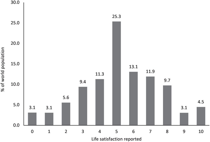
Figure 6.1 Percentage of people in the world at each level of life satisfaction
There is also another way of showing this huge spread of wellbeing – the same facts laid out differently. In Figure 6.2, we break the population down into ten groups of equal size, starting with those who are the least happy on the left of the graph and ending on the right with those who are happiest. As the graph shows, the least happy have an average wellbeing of 1.1 points and the happiest have a wellbeing of 9.2 points. It is a world with many lives that are limited and a few that are truly flourishing. The average wellbeing in the world before COVID-19 was 5.3 points (out of 10) but the spread, as measured by the standard deviation, was 2.3 points.Footnote 3
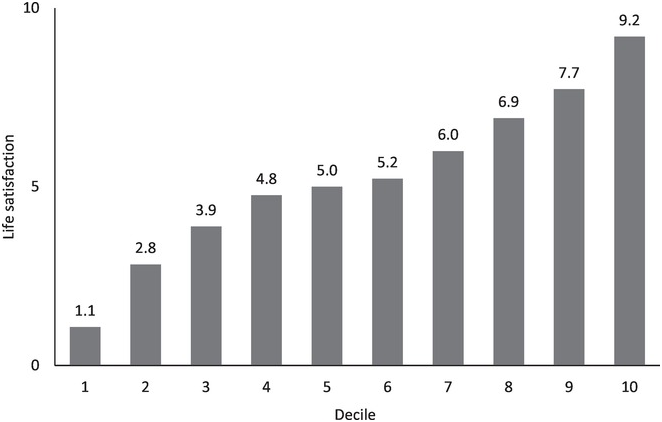
Figure 6.2 Life satisfaction (0–10) of people at each decile of life satisfaction
But how much of this huge spread of wellbeing in the world is due to the spread between countries, and how much of it occurs within countries? The neatest way to answer this question is by taking the square of the standard deviation, known as the variance. We can then partition the variance of individual wellbeing worldwide into two elements:
differences within countries and
differences between countries.
It turns out that the difference between countries contributes only 22% of the overall variance and the main variation (78%) is within countries.Footnote 4 Thus the standard deviation of average wellbeing across countries is about 1.1, while the average of the standard deviation inside a country is about 2.3.
Changes Over Time
It is easy to think that we live in a peculiarly dreadful time. But this is not so, judged by the criterion of wellbeing. There are indeed some countries in which wellbeing declined between 2005–2008 and 2016–2018.Footnote 5 These include the United States, India, Egypt, Brazil, Mexico, Venezuela, South Africa and those affected by civil war. But there are as many countries where wellbeing has risen since 2005–2008 as where it has fallen. Countries where wellbeing rose include both China and most of the countries that were once Communist. Earlier on, between 1980 and 2007, wellbeing rose in more countries than not.Footnote 6 On balance, therefore, the world as a whole is probably as happy as it has ever been.Footnote 7
But progress in wellbeing is by no means automatic, and it is noteworthy that in some important countries, wellbeing is now no higher than it was when records began. In the United States, that means in the 1950s; in West Germany, it means in the 1970s; and in China, it means 1990. We shall discuss this issue more fully in Chapter 13.
By contrast, if we look at short-term changes in wellbeing over the business cycle, wellbeing generally fluctuates up and down around its trend – higher in the boom and lower in the slump. We shall also discuss this issue at length in Chapter 13.
Meanwhile, how has the inequality of wellbeing been changing over time? In most countries, it rose between 2006 and 2018 with especially sharp rises in North America and Sub-Saharan Africa, which now have the highest levels of regional inequality (see Figure 6.3). However, wellbeing inequality fell in Europe, which now has the lowest levels of wellbeing inequality in the world.

Figure 6.3 Trends in the inequality of life satisfaction (0–10) (Standard deviations)
Hedonic Measures of Wellbeing
The analysis so far is based on the Cantril ladder. The Gallup World Poll also asks questions about people’s emotions – the hedonic measures of wellbeing that we discussed in Chapter 1. These questions give useful information about changes over time. At the world level, one can construct an index of positive and negative emotion, based on the question ‘Did you experience X during a lot of the day yesterday?’ For positive emotions, X includes separate questions about happiness, enjoyment, and smiling or laughing. These can be combined into a single index by taking the average proportion of people who said Yes to each question. Similarly for negative emotions – where the questions relate to worry, sadness and anger. Figure 6.4 shows trends at the world level for both positive emotion and negative emotion. As the figure shows, positive affect and the Cantril ladder have been trending down slightly. But negative affect has increased greatly – especially worry. This is confirmed by an additional question on stress where we reproduce the answers for the United States, Western Europe and the world as a whole in Figure 6.5. These findings are deeply troubling. But for the rest of this chapter, we shall revert to measures based on the Cantril ladder.
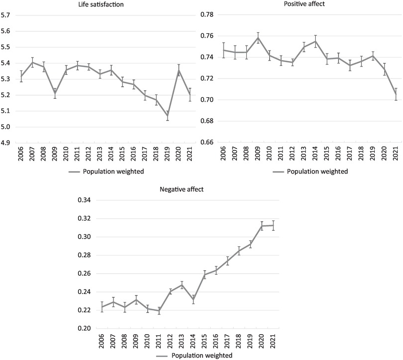
Figure 6.4 Trends in average wellbeing in the world
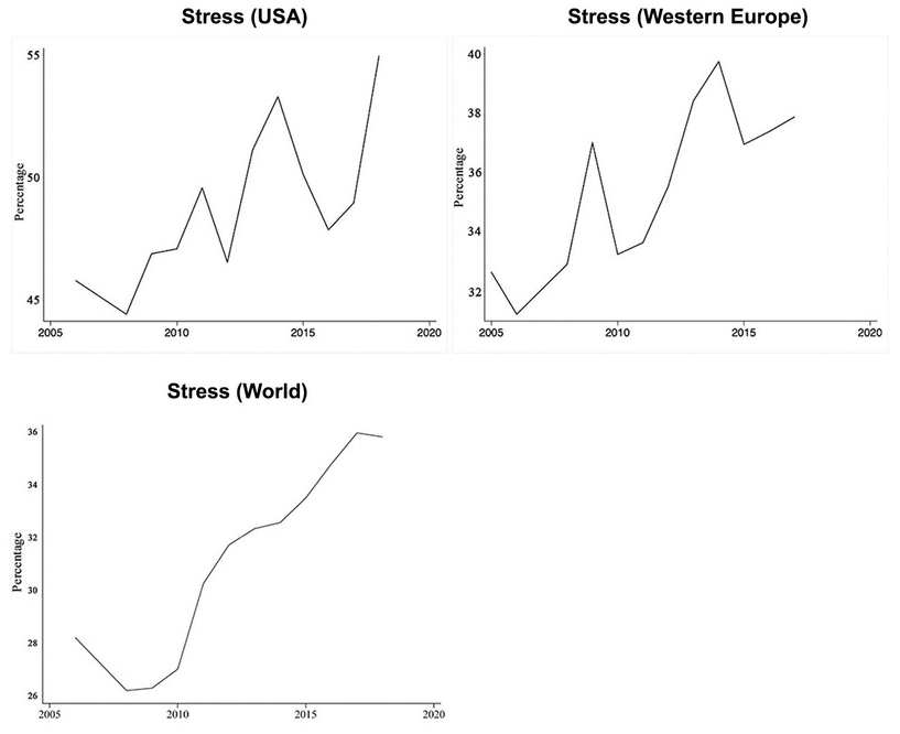
Figure 6.5 Trends in stress (Percentage saying ‘I experienced a lot of stress yesterday’)
Differences Between Groups
So how does average wellbeing differ between groups?
Men and women
Remarkably, the distribution of wellbeing in the world is almost identical for men and women. Women are on average slightly happier than men but the difference is only 0.09 points (out of 10) – one fiftieth of the difference between the happiest and least happy country. Moreover, in almost every country the average wellbeing of men and women is nearly the same, even though wellbeing differs so hugely between countries (see Figure 6.6).Footnote 8
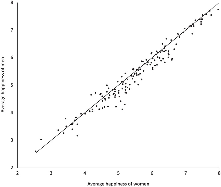
Figure 6.6 Average wellbeing of men and women: By country (the line represents equality)
But what about trends in the relative happiness of men and women? Over the last 50 years, women’s rights in the workplace have been transformed in many countries by legislation requiring equal pay and equal job opportunities. At the same time, women have made huge educational advances relative to men, and through the contraceptive pill have achieved unprecedented control over their fertility. So one might expect that women’s wellbeing would have risen relative to men’s. But has it?Footnote 9
In the United States since the 1970s, both men and women have become less happy, and this has been especially true of white women. In Europe, the situation has been different. Both women and men have become on average more satisfied with their lives, but European women’s happiness has fallen relative to men’s – and this has happened in all 12 countries for which the time series go back as far as the 1970s.
Why is this?Footnote 10 Empirical work has so far failed to produce an explanation. The most likely one (so basic to humans) is social comparisons. As more and more women work, they may increasingly compare themselves with their male colleagues (rather than with other women). And at work women are still frequently at a disadvantage. Another possibility is that women now experience a greater conflict of roles (as compared with men). The US evidence suggests that (up to 2005 at least) there was no change in women’s total work relative to men’s (total time spent in paid work, housework and childcare).Footnote 11 But that is not the same as the sense of responsibility. Women still do more work at home than men, and to that has been added much greater responsibilities at work. Another possibility is family conflict. In the United States, both men and women have become less satisfied with their marriages – and to an equal extent. But satisfaction with marriage affects women’s happiness more than men’s, and increased dissatisfaction with marriage therefore helps to explain the increased gender gap in US happiness.Footnote 12 Finally, there is the enduring fact of male chauvinism. Though this may have diminished over time, the experience of it may have become more intolerable – as the #MeToo movement testifies.
Age
The next issue is Do we become happier as we get older? The effects of aging involve many factors but social factors are among them. As we move into adult life, we take on more responsibility, both in family life and at work. But after some time, we become more established, and any children we had leave home. We relax more. But eventually our health declines. So what is the overall effect of our journey through life?Footnote 13
In most countries, people on average become progressively less happy from their late teens up to their 40s. But then in some countries (including the United States and the UK), they become happier again up to their 70s (before a final decline). Figure 6.7 shows how wellbeing changes over life in each of the world’s regions. Everywhere happiness declines up to around age 40. It then recovers in North America and to a lesser extent in East Asia; in Western Europe, it remains stable; but elsewhere, there are some further declines. (In the former Soviet Union and Warsaw Pact countries the old are markedly less happy, but this is the legacy of the transition and may not continue in future decades).

Figure 6.7 Average life satisfaction: by age, gender and region
Note: NA & ANZ = North America, Australia and New Zealand. CEE & CIS = Central and Eastern Europe and former Soviet Union. LAC = Latin America and Caribbean. MENA = Middle East and North Africa. SSA = Sub-Saharan Africa
So what explains these patterns of wellbeing over the life-course? If age affects wellbeing, it must be through some mediating variables.Footnote 14 But what are they? The first step is to look at the standard variables explaining wellbeing, which we shall consider in Chapter 8. From 20 to 40 years old, most of these variables are moving in the direction that would produce higher wellbeing. So they provide little insight into variation across the life-course.Footnote 15
More light can be found by looking at the Gallup World Poll’s evidence on affect. As we have mentioned, this provides data on negative and positive affect. Beginning with negative emotions (Figure 6.8), stress rises sharply up to middle age and then declines. So does anger, though less markedly. These declines after middle age are especially marked in North America and Western Europe. By contrast, worry, sadness, depression and pain rise steadily through life, but as time passes they become balanced by declining stress and anger. Turning to positive emotions (Figure 6.9), happiness, enjoyment, smiling and interest fall steadily throughout life. In addition, as people age, they are less likely to report that they have someone they can rely on in times of need. People do however feel more rested.

Figure 6.8 Negative Experiences: By age and gender (World)

Figure 6.9 Positive Experiences: By age and gender (World)
Ethnic differences
What about the differences between ethnic groups? In every society, most minority ethnic groups have lower average wellbeing than the majority group. But these differences can be reduced or even eliminated by policy action, such as
reducing gaps in education and income,
banning discrimination in employment and housing,
punishing severely both racially motivated crime and incitement to racial hatred and
improving the respect shown to all (by citizens, by the police, and by the law).
With such action, things can change. For example, the United States has seen substantial improvement in the wellbeing of ethnic minorities, while at the same time the average wellbeing of whites has declined.Footnote 16 This is shown in Figure 6.10, which is based on the General Social Survey. (The happiness scores used are very happy – 3; pretty happy – 2; not too happy – 1.) As Figure 6.10 shows, the gap in happiness between white and black citizens has fallen sharply.Footnote 17

Figure 6.10 Average wellbeing (1–3) of different racial groups in the United States
However, America still has serious ethnic problems, as the Black Lives Matter movement testifies. And so have most other countries, though the groups involved differ widely. In some countries, ethnic tensions lead to civil war.
The Wellbeing of Children
So much for adults; but what about children? In both 2015 and 2018, the OECD surveyed the wellbeing of 15-year-olds in their regular Programme for International Student Assessment (PISA). The question asked was on life satisfaction (0–10) and the survey covered most OECD countries and a number of others. The results by country are in Table 6.1.
Table 6.1 Average life satisfaction of 15-year-olds (0–10)
| OECD Countries | Other countries | |||
|---|---|---|---|---|
| Mexico | 8.11 | Kazakhstan | 8.76 | |
| Colombia | 7.62 | Albania | 8.61 | |
| Finland | 7.61 | Kosovo | 8.30 | |
| Lithuania | 7.61 | North Macedonia | 8.16 | |
| Netherlands | 7.50 | Belarus | 8.10 | |
| Switzerland | 7.38 | Dominican Republic | 8.09 | |
| Spain | 7.35 | Ukraine | 8.03 | |
| Iceland | 7.34 | Costa Rica | 7.96 | |
| Slovak Republic | 7.22 | Saudi Arabia | 7.95 | |
| Estonia | 7.19 | Panama | 7.92 | |
| France | 7.19 | Romania | 7.87 | |
| Latvia | 7.16 | Bosnia and Herzegovina | 7.84 | |
| Austria | 7.14 | Croatia | 7.69 | |
| Portugal | 7.13 | Montenegro | 7.69 | |
| Hungary | 7.12 | Moldova | 7.68 | |
| Luxembourg | 7.04 | Thailand | 7.64 | |
| Chile | 7.03 | Serbia | 7.61 | |
| Germany | 7.02 | Georgia | 7.60 | |
| Sweden | 7.01 | Uruguay | 7.54 | |
| Greece | 6.99 | Indonesia | 7.47 | |
| Czech Republic | 6.91 | Vietnam | 7.47 | |
| Italy | 6.91 | Russia | 7.32 | |
| Slovenia | 6.86 | Peru | 7.31 | |
| United States | 6.75 | Argentina | 7.26 | |
| Ireland | 6.74 | Baku (Azerbaijan) | 7.24 | |
| Poland | 6.74 | Philippines | 7.21 | |
| Korea | 6.52 | Bulgaria | 7.15 | |
| Japan | 6.18 | Brazil | 7.05 | |
| United Kingdom | 6.16 | Malaysia | 7.04 | |
| Turkey | 5.62 | Morocco | 6.95 | |
| Jordan | 6.88 | |||
| United Arab Emirates | 6.88 | |||
| Qatar | 6.84 | |||
| Lebanon | 6.67 | |||
| China | 6.64 | |||
| Malta | 6.56 | |||
| Chinese Taipei | 6.52 | |||
| Hong Kong (China) | 6.27 | |||
| Macao (China) | 6.07 | |||
| Brunei Darussalam | 5.80 |
As can be seen, among the OECD countries the lowest levels of satisfaction were in Turkey, the UK and Japan. The United States was also near the bottom of the list. As so often found, Finland was near the top. Among non-OECD countries, satisfaction was noticeably high in Latin America and post-Communist countries. In most countries, 15-year-old boys were on average happier than 15-year-old girls, with 72% reporting scores of 7 or above compared with only 61% for girls. In most countries, satisfaction was higher among young people from advantaged backgrounds and slightly higher for people from non-immigrant households.
Over time, between 2015 and 2018, young people became less satisfied in every country surveyed (except South Korea). This is a remarkable fact. The average fell by 0.3 points (from 7.3 to 7.0). But the fall was particularly striking in the UK (0.8 points) and in the United States, Japan and Ireland (0.6 points).
Life Expectancy and WELLBYs
Finally, we need to bring into play a completely different dimension – the length of life. As we argued in Chapter 2, the ultimate test of a society’s success is not only the wellbeing that people experience but also the number of years for which they experience it. In other words, what we care about is the number of Wellbeing-Years (or WELLBYs) per person born.Footnote 18
There is, of course, no direct and meaningful way of measuring, at a point in time, the length of people’s lives. But statisticians measure life-expectancy at a point of time as the years a person born now would live if age-specific mortality rates remained as they are now. So a natural measure of the current success of a society is given by

This is not, of course, an appropriate maximand for policy, which should also involve the future wellbeing of those alive and those not yet born. But it is an interesting measure of where we are now.
Table 6.2 provides this assessment for each region of the world for 2017/19 (before COVID-19) and also for 2006/8 (the first available date). As the table shows, average current wellbeing fell slightly between the two periods, especially in South Asia, the Middle East/North Africa and North America. But life-expectancy rose everywhere, above all in Sub-Saharan Africa where it rose by an astonishing seven years. Thus the average WELLBYs per citizen born in the world rose from 369 (5.4 × 68.7) to 373 (5.2 × 72.4). The increase was especially large in the post-Communist regions. But in South Asia, the Middle East/North Africa and in North America there was a fall in current social welfare.
Table 6.2 Trends in wellbeing, life expectancy and social welfare
| Average wellbeing per year | Life expectancy (in years) | Social welfare (WELLBYs per person) | |||||
|---|---|---|---|---|---|---|---|
| 2006/8 | 2017/19 | 2006/8 | 2017/19 | 2006/8 | 2017/19 | Change | |
| World | 5.4 | 5.2 | 68.7 | 72.4 | 369 | 373 | 4 |
| N America | 7.3 | 7.0 | 78.6 | 79.5 | 576 | 556 | −21 |
| S America | 6.2 | 6.1 | 73.4 | 75.3 | 455 | 463 | 8 |
| W Europe | 6.9 | 6.8 | 80.3 | 82.2 | 550 | 561 | 11 |
| C+E Europe | 5.4 | 6.1 | 74.6 | 77.4 | 402 | 488 | 66 |
| Former Soviet Union | 5.2 | 5.4 | 67.5 | 72.2 | 352 | 393 | 41 |
| S E Asia | 5.1 | 5.4 | 69.4 | 72.5 | 354 | 391 | 37 |
| E Asia | 4.9 | 5.2 | 74.8 | 77.8 | 369 | 408 | 39 |
| S Asia | 5.1 | 4.0 | 65.7 | 69.5 | 334 | 278 | −56 |
| M E + N Africa | 5.3 | 4.9 | 71.9 | 74.6 | 380 | 364 | −16 |
| Sub-Saharan Africa | 4.5 | 4.5 | 53.6 | 60.7 | 240 | 271 | 31 |
Conclusions
(1) Wellbeing varies hugely in the human population. Over a sixth of the world’s population has wellbeing of 3 or below (out of 10) – a condition of serious misery. And another sixth has wellbeing of 8 or above.
(2) About 80% of this variance of wellbeing worldwide is within countries and about 20% is between countries.
(3) Between 1980 and 2007, average wellbeing rose in more countries than where it fell. But since 2008, wellbeing has fallen in roughly the same number of countries as where it has risen. Notable falls in wellbeing have been in India, the United States and the Middle East/North Africa. In the US average wellbeing is no higher than it was in the 1950s and the inequality of wellbeing is one of the highest in the OECD.
(4) In most countries, the inequality of wellbeing has increased since 2008, except in Europe, which now has lower inequality than any other region.
(5) Since 2006/8 there has been a large increase in negative affect and in stress.
(6) Average wellbeing is very similar for men and women in almost every country. It declines with age in most parts of the world but in North America and Europe it improves after mid-life. Average wellbeing is below average for most ethnic minorities in most countries.
(7) Children’s wellbeing fell substantially between 2015 and 2018 especially in the UK, the United States and Japan, countries where the wellbeing of 15-year-olds is lower than in most other OECD countries.
(8) Meanwhile, adult life-expectancy has risen in all regions of the world, especially in Sub-Saharan Africa. So the Wellbeing-Years (WELLBYs) that a person now born can expect have increased since 2006–2008 in all regions of the world except South Asia, the Middle East/North Africa and North America.
The rest of Part III of this book attempts to explain some of these facts – both the level of wellbeing and its inequality in the human population. But first we have to sort out the tools we need for this purpose.
Questions for discussion
(1) Do you believe the patterns of wellbeing portrayed in this chapter?
(2) You may want to develop hypotheses about what causes these facts.

There are three kinds of lies: lies, damned lies, and statistics.
To explain the level and inequality of wellbeing, we use the standard tools of quantitative social science. These are mainly the techniques of multiple regression. In this chapter, we shall show how multiple regression can address the following issues.Footnote 1
(1) What is the effect of different factors on the level of wellbeing (using survey data)?
(2) What problems arise in estimating this and how can they be handled?
(3) How far do different factors contribute to the observed inequality of wellbeing?
(4) How can experiments and quasi-experiments show us the effect of interventions to improve wellbeing?
So suppose that a person’s wellbeing (W) is determined by a range of explanatory variables
(X1, …, XN) in an additive fashion. But in addition there is an unexplained residual (e), which is randomly distributed around an average value of zero. Then the wellbeing of the ith individual (Wi) is given by

which we can also write as
 (1)
(1)In this equation, wellbeing is being explained by the Xjs. So wellbeing is the ‘dependent’ variable (or left-hand variable) and the Xjs are the ‘independent’ or (right-hand) variables. These right-hand variables can be of many forms. They can be continuous like income or the logarithm of income or like age or age squared. Or they can be binary variables like unemployment: you are either unemployed or not unemployed. These binary variables are often called dummy variables and they take the value of 1 when you are in that state (e.g., unemployed) and the value of 0 when you are not in that state (e.g., not unemployed).
If we want to explain wellbeing, we have to discover the size of the effect of each thing that affects wellbeing. In other words, we have to discover the size of the ajs. For example, suppose
 (2)
(2)From Chapter 8, you will find as benchmark numbers that a1 = 0.3 and a2 = −0.7. This means that when a person’s log Income increases by one point, her wellbeing increases by 0.3 points (out of 10). Similarly, when a person ceases to be unemployed, her wellbeing increases by 0.7 points (ignoring any effect of a simultaneous change in income). And, if both things happen together, wellbeing increases by a whole point (0.3 + 0.7).
Estimating the Effect of a Variable
But how are we to estimate, as best we can, the true values of these aj coefficients? The best unbiased way of doing this is to find the set of ajs that leaves the smallest sum of squared residuals ei2, across the whole sample of people being studied.Footnote 2 This is known as the method of Ordinary Least Squares (OLS). Standard programmes like STATA will do it for you automatically. However, there are 4 possible problems with such estimates when obtained from a cross-section of the population.
Omitted variables
Suppose that equation (2) is not the correct model but that another X variable should also be in the equation. Suppose, for example, that the right model is
 (3)
(3)where Education means years of education. Clearly education and income are positively correlated. So if a1 and a3 are positive, people with higher income will be getting higher wellbeing for 2 reasons:
the direct effect of income (a1) and
the effect of education in so far as it is correlated with income.
Thus, equation (2) will give an exaggerated estimate of the direct effect (a1) of income on wellbeing.Footnote 3 To leave out education is to leave out a confounding variable. And any such confounding variable must have two properties:
it is causally related to the dependent (LHS) variable and
it is correlated with an independent (RHS) variable.
If we lack data on the confounding variable, the classic way to overcome this problem is to use time-series panel data on the same people. Provided the omitted variable is constant over time, it can cause no problem, since we can now estimate how changes in income within the same person affect changes in her wellbeing. Thus, if we use time-series data, we cease to compare different individuals at the same point of time and we compare the same individual at different periods of time. Algebraically, we do this by expanding equation (2) to include multiple time periods (t) and adding a fixed effect dummy variable (fi) for each individual. This picks up the effect of all the fixed characteristic of the individual (which for most adults will include education). Thus, we now explain the wellbeing of the ith person in the tth time period by
 (4)
(4)There are standard programmes for including fixed-effects. A similar method to this is used for analysing the effect of experiments, but we shall come to this later.
Reverse causality
However, there is another problem. Suppose we are interested in the effect of income on wellbeing. But suppose that there is also the reverse effect – of wellbeing on income.Footnote 4 How can we be sure that, when we estimate equation (2), we are really estimating the effect of income on wellbeing rather than the reverse relationship or a mixture of the two? In other words is equation (2) in principle ‘identifiable’?
For an equation to be identifiable, it must exclude at least one of the variables that appears in the second relationship (the one that determines income).Footnote 5 But, even if it is identifiable, there is still the problem of getting a causal estimate of the effects of the endogenous variable.
The aim has to be to isolate that part of the endogenous variable that is due to something exogenous to the system. A variable that can isolate that part of the endogenous variable is called an instrumental variable. For example, if tax rates or minimum wages changed over time, these would be good instruments. Instrumental variables can also be used to handle the problem of omitted variables. In every case a good instrument
(i) is well related in a causal way to the variable it instruments and
(ii) should not itself appear in the equation, (i.e., it is not correlated with the error term in the equation).
There are programmes for the use of instrumental variables (IVs).
Another way to isolate causal relationships is through the timing of effects. For example, income affects wellbeing in the next period rather than the current period. We can then identify its effect by regressing current wellbeing on income in the previous period. Similarly with unemployment. This gives us
 (5)
(5)Measurement error
Another source of biased estimates is measurement error. If the left-hand variable has high measurement error, this will not bias the estimated coefficients aj. But, if an explanatory variable Xj is measured with error, this will bias aj towards zero. If the measurement error is known, this can be used to correct for the bias. But, if not, an instrumental variable can again come to the rescue, provided it is uncorrelated with the measurement error in the variable it is instrumenting.
Mediating variables
A final issue is this. A multiple regression equation such as (3) shows us the effect of each variable upon wellbeing holding other things constant. But suppose we are interested in the total effect of changing one variable upon wellbeing. For example, we might ask What is the total effect of unemployment upon wellbeing?
The total effect is clearly
a2, plus
a1 times the effect of unemployment upon log income.
That is one way you could estimate it. An alternative way is to take equation (2) and leave income out of the equation, so that the estimated coefficient on unemployment includes any effect that unemployment has on wellbeing via its effect on income.
In a case like this, income is a mediating variable. If we are only interested in the total effect of unemployment, we can simply leave the mediating variable out of the equation. Or we can estimate a system of structural equations consisting of (2) and the equation that determines income. This discussion brings out one crucial point in wellbeing research. We should always be very clear what question we are trying to answer. We should choose our equation or equations accordingly.
Standard errors and significance
All coefficients are estimated with a margin of uncertainty. Each estimated coefficient has a ‘standard error’ (se) around the estimated value. The true value will lie within 2 ‘standard errors’ on either side of the estimated coefficients in 95% of samples. Thus the ‘95% confidence interval’ for the αj coefficient runs from  , where
  means the estimated value of αj. If this confidence interval does not include the value zero, the estimated coefficient is said to be ‘significantly different from zero at the 95% level’.
For many psychologists, this issue of significance is considered crucial. It answers the question ‘Does X affect W at all?’ But for policy purposes the more important question is ‘How much does X affect W?’ So the coefficient itself is more interesting than its significance level. For any sample size, the estimated coefficient is the best available answer to the question of how much X changes W. And, if you increase the size of the sample, the expected value of the estimated aj does not change but its standard error automatically falls (it is inversely proportional to the square root of the sample size). So in this book we focus more heavily on the size of coefficients than on their significance (though we sometimes show standard errors in brackets in the tables).
The question we have been asking thus far in this chapter is How does wellbeing change when an independent variable changes? In algebraic terms, we have been studying dW/dXj? This is the type of number we need in order to evaluate a policy change. For example, suppose we increased the income of poor people by 20%, how much would their wellbeing change (on a scale of 0–10)? If aj = 0.3, it would increase by 0.06 points (0.3 × 0.2). A quite different question is In which areas of life should we look hardest in the search for better policies?
The Explanatory Power of a Variable
If our main aim is to help the people with the lowest wellbeing (as we discussed in Chapter 2), then our focus should be on what explains the inequality of wellbeing. To see why, suppose first that wellbeing depends only on one variable X1, with W = α0 + α1X1. Then the distribution of W depends only on the distribution of X1. If W is unequal, it is because X1 is unequal and α1 is high. The higher the standard deviation (σ1) of X1 and the higher α1, the greater the inequality of W. This is illustrated in Figure 7.1. For high variance of W, the numbers in misery correspond to the areas A and B. But for the low variance of W the numbers in misery correspond only to the area B.

Figure 7.1 How the numbers in misery are affected by a1σ1
A next natural step is to compare the standard deviation of a1σ1 with the standard deviation of wellbeing itself. Obviously, if they were equal in size, the spread of X1 would be ‘explaining’ the whole spread of wellbeing σw – in other words, the two variables would be perfectly correlated. The correlation coefficient (r) between W and X1 is therefore a1σ1/σw:

However, this can be either positive or negative depending on the sign of a1. So a natural measure of the explanatory power of a right-hand variable is the squared value of r (which is also often written as R2):

Since the denominator is the variance of wellbeing, this shows what proportion of the variance in wellbeing is explained by the variance of X1.
In the real world, wellbeing depends on more than one variable (see equation [1]). The policy-maker may then ask Which of these variables is producing the largest amount of misery?Footnote 6 For this purpose, we need to compare the explanatory power of the different variable. This is done by computing for each variable its partial correlation coefficient with wellbeing. This partial correlation coefficient is normally described as βj where

This β-coefficient will appear frequently throughout this book.Footnote 7
These β-coefficients are hugely interesting, as we shall see via two steps. First, starting from equation (1) we can readily derive the following equation.Footnote 8
 (6)
(6)Here we have standardised each variable by measuring it from its mean and dividing it by its standard deviation. These standardised equations appear many times in this book.Footnote 9
But, to see the importance of these βs, we move on to a second equation, which is derived from (6).Footnote 10 This says
 (7)
(7)r2 is the proportion of the variance of W that is explained by the right-hand variables. And rgk is the correlation coefficient between Xg and Xk.
Thus, the left-hand side is the share of the variance of wellbeing that is explained. The right-hand side consists of Σβj2, which includes all the effects of the independent variation of the Xjs, plus the effects of all their covariances. Thus βj (or the partial correlation coefficient) measures the explanatory power of a variable (just as the correlation coefficient does in a simple bivariate relationship).
But some readers may wonder if this approach can handle independent variables that are binary. It can, because the standard deviation of a binary variable is simply  , where p is the proportion of people answering Yes to the binary question. For example, the standard deviation of Unemployed is
  where u is the unemployed rate. Thus, if Xj is Unemployed, its β coefficient is
 .
.
Binary dependent variables
The matter is more complicated when it is the dependent variable that is binary. For example, suppose we divide the population into those who are in misery (with wellbeing below say 6) and the rest. How can we handle this? The most natural approach is, as normal, to regress the binary variable on all the other variables. This is what we often do in this book and, since it provides statistics of the standard kind, it is easy to understand.Footnote 11
Box 7.1 Odds ratios
In analysing the effect of one binary variable on another binary variable, psychologists and sociologists often use the concept of an ‘odds ratio’ rather than the values of aj and βj we have been discussing. Suppose, for example, we ask: How much more likely are unemployed people to be in misery, compared with people who are not unemployed? Imagine 100 people were distributed as follows (Table 7.1):
Table 7.1 Distribution of 100 people by unemployment status and misery status
| In misery | Not in misery | Total | |
|---|---|---|---|
| Unemployed | 2 | 8 | 10 |
| Not unemployed | 9 | 81 | 90 |
| Total | 11 | 89 | 100 |
In this situation, the chance of an unemployed person being in misery is much higher than the chance of a non-unemployed person being in misery. The odds-ratio is

But odds ratios do not answer either of the main questions we are addressing in this chapter. First, if we are interested in the effect on wellbeing of reducing unemployment, the proper measure of this effect is not the odds ratio but the absolute difference in the probabilities of misery between unemployed and non-unemployed people, that is, 0.2−0.1 = 0.1. Second, if we are interested in the power of unemployment to explain the prevalence of misery, the correct statistic is the correlation coefficient between the two. So we shall not be showing odds ratios in this book, though the reader is able to compute them, given the necessary information.
Effect size of a binary independent variable
We have so far considered two ways in which to report regression results. One is to report the absolute effect of say unemployment on wellbeing in units of wellbeing. The other is to look at the relationship when both variables are standardised. However, there is the third approach that is often useful. This is to measure only the dependent variable in a standardised fashion. For example, we might ask ‘When a person becomes unemployed, by how many standard deviations does his wellbeing go down?’ This is a measure known as the effect size of the independent variable (sometimes knows as Cohen’s d):

This is particularly useful when reporting the effect of an experiment.Footnote 12
Experiments
So far, we have been discussing the use of naturalistic data – mainly obtained by surveys of the population. As we have mentioned, it is often difficult to establish the causal effect of one variable on another from this type of data. The simplest way to establish a causal relationship is through a properly controlled experiment. Moreover, if you want to examine the effect of a policy that has never been tried before, it is the best way to get convincing evidence of its effects.
So how do we estimate the effects of being ‘treated’ in an experiment? Let’s begin with a simple example. Suppose we want to try introducing a wellbeing curriculum into a school. Our aim is to see whether it makes any difference to those who receive it. So we would select two groups of pupils who were as similar to each other as possible. Then we would give the wellbeing curriculum to the treatment group (T) but not the control group (c). We would also measure the wellbeing of both groups before and after the treatment. So we would have the following values of wellbeing for each of four situations (Table 7.2).
Table 7.2 Average wellbeing of each group before and after the experiment
| Before | After | |
|---|---|---|
| Treatment group (T) | WT0 | WT1 |
| Control group (C) | WC0 | WC1 |
To find the average effect of the treatment, we would compare the change in wellbeing experienced by the treatment group (T) with that experienced by the control group (C). Thus, the ‘average treatment effect on the treated’ (ATT) would be estimated as
 (8)
(8)In other words, the ATT is the ‘difference in differences’, or for short the ‘diff in diff’.
There may of course be many ways in which both groups changed between periods 0 and 1 – they will become older, they may experience a flu epidemic or whatever. But those changes should be similar for both groups. Thus the only observable thing that can produce a different change in wellbeing is the fact that Group T took the course and Group C did not.
Of course, there may also be some unobservable difference in experience, which means that the ATT is always estimated with a standard error. So, to put things into a more general form, let’s imagine we have observations over a number of years. We then estimate
 (9)
(9)Here Tit is a variable which takes the value 1 in all periods after someone has taken the course, vt is a year dummy, fi is a person fixed effect and eit is random noise.
So far, we have assumed that in our experiment we can easily arrange for the treatment group and the control group to be reasonably similar. This is never in fact completely possible. But the method that gets us closest to it is ‘random assignment’.Footnote 13 In this case, we select an overall group for the experiment and then randomly assign people to either Group T or Group C (e.g., by tossing a coin for each individual). In this way, the groups are more likely to be similar than in any other way. Of course we can then check whether they differ in observable characteristics (X) and we can then allow in our equation for the possibility that these variables affect the measured ATT. Our equation then becomes
 (10)
(10)Estimating equations like this are quite common.
However, randomisation between individuals is often not practicable. For example, suppose you wanted to test whether higher income transfers raised wellbeing enough to justify the cost. You could not randomly allocate money within a given population – it would be considered unfair since the transfer clearly benefits the recipient. You might, however, choose to transfer money to all eligible people in some areas and not in others, with the allocation between areas being random. This might not be considered unfair. Similarly, suppose you wanted to test the effects of improved teaching of life-skills in schools. Within a school it might be organisationally impossible to give improved teaching to some children and not others – or even to some classes. But you could use random assignment across schools. Or you could even argue that it is ‘quasi-random’ whether a child is born in Year t or Year t − 1; in this case, you could use children born in year t as a control group in the trial of a treatment applied to those born in year t + 1 (see Chapter 9). So all experiments should, if at all possible, use randomisation to reduce the unobservable differences between the treatment and control groups.
Selection bias
But suppose an innovation is made without an experiment and we then want to know its effects. For example, an exercise programme has been established, which some people have decided to adopt. Has it done them any good?
The only information that we have is for the period after the innovation. But we do also have information on people who did not opt in to the programme. So, can we answer our question by comparing the wellbeing of those who took the programme with those who didn’t? Probably not, because the people who opted into the programme may have differed from those who didn’t: they may well have started with higher wellbeing in the first place. So, if we just compared their final wellbeing with those of non-participants, the difference could be largely due to ‘selection bias’.
One method to deal with this is called Propensity Score Matching. In it we first take the whole sample of participants and non-participants and do a logit (or probit) analysis to identify that equation that best predicts whether they participate or not. From this analysis, we can say for every participant what was the probability they participated. We then find, for each participant, a non-participant with the same (or nearly the same) probability of participating. It is those non-participants who become the control group and we now compare their wellbeing with that of the treatment group. This gives us our estimate of the average treatment effect on the treated:
 (11)
(11)Summary
(1) If W = a0 + ∑aj Xj +e, then the best unbiased way to estimate the values of the ajs is by Ordinary Last Squares (choosing the ajs to minimise the sum of squared residuals e2).
(2) Omitted variables are confounders that can lead to biased estimates of the effect of the variables which are included.
(3) Time series estimation can eliminate any problem caused by omitted variables which are constant over time. Time series can also help to identify a causal effect if this takes place with a lag, so that for example Xt-1 is affecting Wt.
(4) If a right-hand variable is endogenous, it should if possible be instrumented by an instrumental variable that is independent of the error in the equation. Instrumental variables can also help with omitted variables and measurement error.
(5) If an explanatory variable is measured with error, its estimated coefficient will be biased towards zero. This problem can again be solved by using an instrumental variable uncorrelated with the original measurement error.
(6) All regression estimates are estimated with ‘standard errors’ (se). The 95% confidence interval is the coefficient ± 2 se. Provided this interval does not include zero, the coefficient is ‘significantly different from zero at the 95% level’. But the coefficient estimate is more interesting that its significance.
(7) To find the explanatory power of the different variables, we run the equation using standardised variables, that is, the original variables minus their mean and divided by their standard deviation. The resulting coefficients (βj) – or partial correlation coefficients – reflect the explanatory power of the independent variation of each variable Xj. They are equal to ajσj/σw where w is the dependent variable.
(8) The surest way to determine a causal effect is by experiment. The best form of experiment is by random assignment. We then measure the wellbeing of the treatment and the control group before and after the experiment. This difference-in-difference measures the average treatment effect on the treated.
(9) Where random assignment is impossible, naturalistic data can be used and the outcome for the treatment group compared with a similar untreated group chosen by Propensity Score Matching.
(10) If the measured effect of a treatment is a (in units of the outcome variable W), the ‘effect size’ is a/σw.
We can now put these tools to work.

Happy the man who has learned the cause of things …
We can now put these tools to use in explaining the huge inequalities that exist in wellbeing. These inequalities are interesting in themselves. And they also provide naturalistic evidence that helps us to predict how policies of different kinds would change people’s wellbeing.Footnote 1 So this chapter applies the tools presented in Chapter 7 to explain and learn from the differences in Chapter 6.
We proceed as follows:
First, we outline a framework for how adult wellbeing is determined within a country.
Next, we take adult wellbeing differences within a country and see how these are explained by differences in adult characteristics.
Then we go back to childhood and see how well the child predicts the adult.
Finally, we look at the role of social norms and institutions and study their effects by looking at differences between countries.
This chapter is very important in setting the framework for the rest of Part III of the book – which looks at each influence in much more detail.
Wellbeing and the Life Cycle
Our adult wellbeing is the product of our whole life to date (see Figure 8.1). Our early development is affected first by our parents (including their genes) and then by our schooling. These are the main factors that determine our outcomes up to the end of childhood. These outcomes then help to predict our adult outcomes, which in turn determine our adult life satisfaction. In what follows, we shall work backwards, looking first at the role of adult outcomes, then at the role of child outcomes and finally (in Chapter 9) at the role of family and schooling.

Figure 8.1 How adult wellbeing is determined
Note: Earlier factors also influence later outcomes directly
Personal Determinants of Adult Wellbeing
There have been thousands of studies of the personal causes of adult wellbeing. But they are difficult to compare because they use different measures of wellbeing and they study the effect of different sets of determinants. We shall therefore focus in this chapter on one study that used a single measure of wellbeing (life satisfaction) and looked at all the main influences simultaneously.Footnote 2 The main influences included were:
Physical health (number of illnesses)
Mental health (has ever been diagnosed with depression or an anxiety disorder)
Is unemployed (versus employed)
Quality of work (index)
Family
Has partner (versus single)
Is separated (versus single)
Is widowed (versus single)
Education (years)
Many studies of wellbeing do not include mental health as an explanatory factor, since it is itself a feeling. But this is why we do not include self-reported feelings as measures of mental health – instead, we include an objective diagnosis by a third party. The question used is ‘Have you ever been told by a doctor, nurse of other health professional that you had an anxiety disorder and/or depressive disorder?’ Since most such experiences are prior to being surveyed, they are essentially measuring something exogenous. Besides, it would be quite wrong not to include mental illness as an explanation for wellbeing, when this is such an important issue for so many people, independently of the other right-hand variables. As the equations that follow show, low wellbeing is not the same as mental illness and can be caused by many other factors besides mental illness.
So the task is to estimate equation (1) in Chapter 7, with current life satisfaction as the dependent variable and the variables listed above as the independent variables. The equation estimated is cross-sectional – a point to which we shall return. The study covered Britain, Germany, Australia and the United States, with broadly similar results from all four countries. The results we report in Table 8.1 come mainly from a British survey (Understanding Society). But the mental health coefficient is from the United States and Australia (where the measure of mental health is more exogenous and the results are very similar). And the quality of work result comes from a different study using the European Social Survey.Footnote 3
Table 8.1 How different factors affect life satisfaction (0–10) of adults over 25 (Britain) (Pooled cross section) (R2 = 0.19)
| Effect on life satisfaction (0–10) | |
|---|---|
| Physical health problems (No. of illnesses) | −0.22 (0.01) |
| Mental health problems (0,1) | −0.72 (0.05) |
| Unemployed (versus employed; 0,1) | −0.70 (0.04) |
| Quality of work (effect of 1SD) | +0.40 (0.04) |
| Partnered (versus single; 0,1) | +0.59 (0.03) |
| Separated (versus single; 0,1) | −0.15 (0.04) |
| Widowed (versus single; 0,1) | +0.11 (0.08) |
| Income (log) | +0.17 (0.01) |
| Education (years) | +0.03 (0.00) |
Notes: Control variables include comparators’ income, education, unemployment and partnership, as well as gender, age and age squared and year fixed effects. Standard errors in brackets.
Table 8.1 shows, for example, that people ever diagnosed with mental illness are currently (other things equal) less satisfied with their life by 0.72 points.Footnote 4 Unemployment has a similar effect, as does not having a partner. A unit increase in log income increases wellbeing by 0.17 points, which means that the doubling of income raises wellbeing by 0.12 points.Footnote 5 Note that the standard error (in brackets) of these coefficients are small relative to the coefficients themselves, so the estimates are fairly well defined and significantly different from zero at the 95% level.
From Table 8.1, we learn the effect of each variable upon wellbeing. But this does not tell us how far the inequality of that variable explains the inequality of wellbeing. For that purpose, we have to multiply the effect of each explanatory variable by its own standard deviation – and then divide it by the standard deviation of wellbeing. This gives us the βj measure discussed in Chapter 7 – recall that βj = ajσj/σw.
In Figure 8.2, we give these β values in graphical form. To simplify the display, we have treated every variable as if it had a positive β – by, for example, relabelling Unemployed as Not unemployed.

Figure 8.2 What explains the variation of life satisfaction among adults over 25? (Britain) Partial correlation coefficients (β) (R2 = 0.19).
Notes: For quality of work see their chapter 4. Standard errors in brackets
Notice first that the whole equation has an R2 of 0.19 – we are only explaining 19% of the total variance. It is very important not to over-claim explanatory power.Footnote 6 And it is also quite wrong to label the unexplained residual as ‘luck’. It is quite simply the variation in wellbeing that we have not been able to explain or is due to measurement error. Nevertheless, what we do know is that health is extremely important (especially mental health). Work is also important – having it (if you want it) and its quality. Family life also matters.
So does income, but its explanatory power is no higher than many other variables. In Figure 8.2 it explains under 1% of the variance of life satisfaction, since its β2 value is under 0.12. But as we shall see in Chapter 13, the figure can rise to 3% in some countries – but still no higher than some other influences.
Before we accept this conclusion, we have to ask some of the questions we discussed in Chapter 7. First, is there a problem of measurement error? This is unlikely to affect the ranking of income in Figure 8.2 since income is measured more accurately than many of the other variables. Second, are there important omitted variables or problems of endogeneity? To investigate these problems, we can use the panel data to perform a fixed-effects analysis as in Equation (7.4). In panel regressions, all the coefficients are reduced, partly because the problem of measurement error becomes more acute. The coefficients on income fall more than most, though this may be partly because the exact timings are not well caught by the data. For this chapter, we stick to cross-sectional results; but in Chapter 13 we also give the results of fixed effects regressions.
It is important to stress that for all the variables in Table 8.1 and Figure 8.2, the coefficients reflect the effect of the variable, other things constant. If we wanted to investigate the total effect of income on wellbeing, we would also have to include its effects through other ‘mediating’ variables like having a partner. This is quite difficult to compute. But it is easy to compute a maximum value for the total coefficient on income (or any other variable). It is the simple bivariate coefficient, which in this case is about double the coefficient holding other things constant.
Another obvious question is this: Doesn’t income explain more of the prevalence of low wellbeing than is implied by Figure 8.2? To investigate this, we construct a new variable. This is a simple binary variable for misery (M), which is constructed as follows:Footnote 7
M equals 1 if wellbeing is 5 or below
M equals 0 if wellbeing is above 5
Misery (thus defined) affects the bottom 10% or so of the British population – so it is a good measure of deprivation. We can then run the following simple equation:

If we take averages across all individuals, this equation predicts the proportion of people in misery, which is given by

In an analysis for Britain, Australia and the United States, mental health problems accounted for more of the misery than any other factor.Footnote 8 In Britain and Australia, this was followed by physical illness, and in the United States by low income. Unemployment, though devastating to those affected, came in lower than health and poverty, because of the smaller numbers affected.
A slightly different question is What best explains who is in misery and who is not? In other words, what are the most important elements in the following relationship:

In Figure 8.3, we show the values of the β coefficients where this time Misery is the dependent variable. As can be seen, these coefficients are slightly smaller than when we are explaining the full continuous range of Life–Satisfaction (in Figure 8.2). This is to be expected. But, strikingly, the relative importance of the different factors is the same whether we are explaining low wellbeing or the whole spread across the spectrum.

Figure 8.3 What explains the variation of misery among adults over 25? (Britain) Partial correlation coefficients (β) (R2 = 0.14)
Note: See Figure 8.2
Childhood Predictors of Individual Wellbeing
So much for the adult causes of adult wellbeing. But aren’t many of the adult influences we have looked at caused by how we were in childhood? They are indeed. There are three main dimensions of child development: intellectual, emotional and behavioural. A big question for schools is ‘Which of these is the best predictor of whether a child will have a satisfying adult life?’
The following analysis is based on a follow-up of all British children born in a week in 1970 (the British Cohort Study 1970). The measures of child development that we use are these:
Intellectual: highest qualification ever obtained
Behavioural: behaviour measured at age 16 (by 17 questions asked to the mother)
Emotional: emotional health measured at age 16 (by 22 questions asked to the young person and 8 to the mother).
As Figure 8.4 shows, the best predictor of a satisfying adult life is not your qualifications but a simple measure of your emotional health at 16. This is an important finding for educational policy since, as Chapter 9 shows, schools have such a huge influence on the wellbeing of their children. Qualifications also matter of course and are by far the best predictor of an adult’s income. But, as we have seen, income is less important for adults than their mental health, which is best predicted by their emotional health in childhood.

Figure 8.4 How adult life satisfaction is predicted by child outcomes (Britain) Partial correlation coefficients (β) (R2 = 0.035)
Note: Adult life satisfaction is average at ages 34 and 42. Controls include family variables. Standard errors in brackets
As we argue in Chapter 9, child wellbeing is important in itself – childhood is a substantial part of our whole life experience. But wellbeing as a child is also the foundation for wellbeing as an adult.
The Effects of Social Norms and Institutions
We have focused so far on what explains the differences in wellbeing between people within the same country. But what explains the differences between countries? There are important social norms and institutions that everyone in a country shares. While we cannot identify these effects by studying people in one country only, we can do it by comparing one country with another. The Gallup World Poll data enable us to do just that – to study the effect of
ethical standards (trustworthiness and generosity),
networks of social support and
personal freedom.
We measure these by the answers in each country to the following questions:
| Trust | Proportion who say Yes to the first half of ‘In general, do you think that most people can be trusted, or alternatively that you can’t be too careful in dealing with people?’ |
| Generosity | Proportion who say Yes to ‘Have you donated money to a charity in the present month?’ |
| Social Support | Proportion who say Yes to ‘If you were in trouble, do you have relatives or friends you can count on to help you whenever you need them?’ |
| Freedom | Proportion who say Yes to ‘Are you satisfied or dissatisfied with your freedom to choose what you do with your life?’. |
We also include the effect of average GDP per head and healthy life expectancy (measured in years).
In the cross-sectional analysis in Table 8.2, we show for each of these variables how average life-evaluation changes when the percentage who say Yes rises from 0 to 100. All four factors have substantial effect. So does healthy life-expectancy – for example, an increase of 10 years raises life evaluation by 0.3 points. And the effect of income across countries is similar to its effect within many countries – a doubling of income raises average life-evaluation by 0.23 points (out of 10).
Table 8.2 How national life satisfaction (0–10) is affected by country-level variables (R2 = 0.77)
| Change | Effect on average life satisfaction (0–10) | |
|---|---|---|
| Trust | 100% v. 0% | 1.08 (.45) |
| Generosity | 100% v. 0% | 0.54 (.41) |
| Social support | 100% v. 0% | 2.03 (.61) |
| Freedom | 100% v. 0% | 1.41 (.49) |
| Income | Doubling | 0.23 (.06) |
| Health | Years of healthy life | 0.03 (.01) |
It is also interesting to see how far the different factors contribute to the actual dispersion of life satisfaction across countries. Here income plays a more conspicuous role due to the huge income differences between countries. Health differences also come through as very important. This can be seen in Figure 8.5, which gives the βj coefficients corresponding to the aj coefficients in Table 8.2. The social norms are also very important. For example, what distinguishes the eight countries with the highest life satisfaction in the world is not their income but their high levels of trust, social support, freedom and generosity.Footnote 9 These are the five Nordic countries as well as the Netherlands, Switzerland and New Zealand (see Table 13.1). The countries at the bottom are mainly the war-torn countries of sub-Saharan Africa and the Middle East (Afghanistan, Syria and Yemen), which not only have poor income and healthcare but are low on the social features that wellbeing requires.Footnote 10

Figure 8.5 How differences in national life satisfaction are explained by country-level variables – partial correlation coefficients (β) (R2 = 0.77)
Conclusions
This concludes our brief initial overview of the main causes of high and low wellbeing – and of the huge variation in wellbeing in the world. All the findings are cross-sectional, with time series and experiments left to later chapters. The findings of this chapter provide the framework for the rest of Part III of the book – starting with personal factors and working outwards to those relating to whole communities.
Within a country (if it is advanced), the main factors explaining the variance of wellbeing (and the prevalence of misery) are in rough order of importance:
mental illness,
physical illness,
having work and the quality of that work,
having a partner,
family income and
education
The variation of wellbeing across countries is largely explained (in rough order of importance) by:
income,
health,
social support,
personal freedom,
trusting social relations and
generosity
Predicting whether a child will become a happy adult is not easy. But the child’s wellbeing is a better predictor of satisfaction in adult life than the child’s academic success is. And as Chapter 9 shows, both schools and parents have big effects on children’s wellbeing.
Questions for discussion
(1) Are the findings about income in Figure 8.2 credible? Could problems of measurement error have produced incorrect rankings?
(2) Is Figure 8.5 informative?

Don’t be too hard on parents. You may find yourself in their place.
We begin our lives in families. After a while we go to school. And eventually most of us form families of our own. How do these experiences affect us?
The Effect of Parents
How our parents treat us makes a huge difference. For humans, we cannot prove this experimentally, but we can for animals – by allocating them randomly to be brought up by different parents. A classic study of rats by Michael Meaney took the offspring of mother rats who were bad at licking their offspring and allocated some of them to foster mothers who were good at licking.Footnote 1 These offspring grew up to be much less stressed, and they also became much better at licking their own offspring. Similarly, a classic study of rhesus monkeys by Stephen Suomi took the offspring of overactive mothers and randomly allocated some of them to calmer foster mothers.Footnote 2 These offspring became much calmer than those who stayed with their biological mothers.
However, we cannot do such experiments on humans. So we have to rely on data thrown up by people’s actual experiences of life. Fortunately, there are now a number of longitudinal studies, which follow the same person from the cradle into adult life, and most of our understanding of the impact of families and schooling comes from these surveys. In each of them, the wellbeing of the children is measured initially by questions to their parents and teachers and then (after about 10) to the children themselves as well. Here are some key findings.
Every child needs unconditional love. The basic need is for a secure emotional tie to at least one specific person. This experience of ‘attachment’ is the basis for an inner security that can last throughout life.Footnote 3 Sixty years ago, the importance of attachment was identified by John Bowlby;Footnote 4 and his idea has stood the test of time quite well. In meta-analyses, early attachment is correlated with later social competence (r = .18), pro-social behaviour (r = .15) and inner wellbeing (r = .08),Footnote 5 and these correlations are undoubtedly underestimates because attachment is so difficult to measure precisely.
A striking illustration of the importance of caring relationships comes from a tragic ‘natural experiment’. After the end of Communism, some Romanian orphans were randomly assigned to foster-care in Western families; the unlucky ones remained in the orphanage. On average, the children were 21 months old when they were assigned one way or the other, and they were assessed again at 4 ½ years of age. If they had been assigned for foster-care, the children’s mental and cognitive wellbeing at 4 ½ was over one half of a standard deviation higher than if they had stayed in the orphanage.Footnote 6 And the younger the age at which the fostering began the better the outcome.
So the love of caregivers is essential. But so too is firmness – the ability to set boundaries. If combined with warmth, this is known as ‘authoritative’ parenting, and it is the most widely recommended approach. In this approach, compliance with rules does not come from fear, but children learn to internalise the parent’s response and thereafter act to please their own ‘better selves’.Footnote 7
Abusive parents can change their children for life, and abuse includes psychological neglect as well as sexual or physical abuse. Though most abused children develop normally, a minority experience long-lasting damage. On average, there are marked brain differences between people who have and who have not been maltreated as children.Footnote 8 Maltreatment also affects behaviour,Footnote 9 but the long-term effects on internal wellbeing are even stronger.Footnote 10
So for a child the relationship to her parents is crucial. But so is the relationship between the parents themselves. At present, 50% of 16-year-olds are in separated families in the United States, and in Britain it is over 40%. How much does this matter?
The literature on child development is large.Footnote 11 However, most of the main findings can be illustrated from within one study, which makes the findings on different influences easier to compare. This is the famous ALSPAC survey of all the children born in or around Bristol, England in 1991/2. Table 9.1 shows how their parents affected the wellbeing of their children – and also their behaviour and their academic performance (all measured at age 16).
Table 9.1 How child outcomes at age 16 are affected by family and schooling – partial correlation coefficients (β)
| Wellbeing at 16 | Behaviour at 16 | Academic score at 16 | |
|---|---|---|---|
| Conflict between parents | −0.04 | −0.14 | −0.02 |
| Mother’s mental health | 0.16 | 0.17 | 0.03 |
| Father’s mental health | 0.04 | – | – |
| Family income (log) | 0.07 | 0.08 | 0.14 |
| Mother’s involvement with child | 0.04 | 0.05 | 0.02 |
| Mother worked (% of 1st year) | – | – | −0.02 |
| Mother worked (% of other years) | – | −0.05 | 0.04 |
| Father unemployed (% of years) | – | – | −0.03 |
| Parents’ education (years) | – | 0.04 | 0.17 |
| Mother’s aggression to child | −0.03 | −0.12 | – |
| All parental variables | 0.27 | 0.31 | 0.35 |
Note: Wellbeing is the average of mother’s and child’s replies to the Short Mood and Feelings Questionnaire. Behaviour is mother’s replies to Strength and Difficulties Questionnaire. Academic score is the General Certificate of Secondary Education (GCSE). Control variables include gender, ethnicity and the name of the primary and secondary school. For questionnaires see Annex 9.1.
As the table shows, family conflict is bad for all three of these outcomes. And, incidentally, for any given level of family conflict, a break-up of the family causes no additional damage, except to academic performance. But ongoing conflict between the parents after they break up increases the risk that the children will become depressed or aggressive. By contrast, seeing more of the absent parent reduces that risk.Footnote 12
Closely related to family conflict is the mental health of the parents. In the Bristol study, the single most important family variable predicting a child’s wellbeing at 16 was the mental health of the mother.Footnote 13 The father’s mental health also mattered but less so – probably because the mother is still, generally, the primary care giver. Clearly poor mental health can lead to family conflict, and vice-versa, but what emerges clearly is that both matter, holding the other constant.
There are three other causal factors that are much discussed. The first is family income. This is much less important for child wellbeing than it is for exam performance. The Bristol study showed that a 10% rise in family income would increase a child’s wellbeing by only 0.007 standard deviations. Similar findings emerge from other studies.Footnote 14 A second important influence is parental involvement in the life of the child. This is important in early life, but in the Bristol study it had few lasting effects. And the third issue is whether the mother works and for how long. In the majority of studies, this has no negative effect on child wellbeing, once the positive effect of the mother’s earnings is taken into account.Footnote 15
As the last row of Table 9.1 shows, the overall effect of all the observed parental characteristics upon the wellbeing of the child is a β-coefficient equal to 0.27.Footnote 16 It is time to compare this with the contribution of schooling.
The Effect of Schools
The Bristol study covered all the children who were born in that area over a 2-year period. As a result, each school in the area taught many children who were in the study. This enables us to see how much difference it made which school a child went to. The results showed that it made a very great difference – the schools really did affect the wellbeing of the children, as well as their behaviour and their exam performance.
The study estimated the following equation for wellbeing (W), as well as similar equations for behaviour and academic score:
 (1)
(1)Here  is the wellbeing of the ith child, and the Xijs are the characteristics of the parents. There is also a 1/0 dummy variable
  for each school (which takes the value 1 when the school is the one the individual attended and otherwise zero). So the coefficient as tells us what difference it made that a pupil went to school s.Footnote 17
We can now ask: How far did these different effects of the different schools contribute to the overall spread of wellbeing in the child population? The answer can be found by looking at the standard deviation of the as coefficients (weighted by pupil numbers) relative to the standard deviation of W. The answers are in Table 9.2. In the first row, the table examines how much difference secondary schools make to children at age 16, holding constant not only all the measured family variables but also the child’s measurement on the same outcome when she entered the school at age 11. The second row does the same for primary schools, showing their effects at age 11 holding constant the measurement of the same outcome at age 8. And the third row shows their effects at age 8 holding constant the measurement of the same outcome at age 7. As Table 9.2 shows, schools make a remarkably huge difference to the wellbeing of their pupils – almost as much a difference as they make to their academic performance. And, looking back at Table 9.1, schools are making as much difference to child wellbeing as parents do (in so far as we can measure parents’ characteristics).
Table 9.2 Standard deviation of school dummy coefficients for different standardised outcomes
| Wellbeing | Behaviour | Academic performance | ||
|---|---|---|---|---|
| Secondary school | Age 16 | 0.26 | 0.21 | 0.29 |
| Primary schools | Age 11 | 0.24 | 0.19 | 0.27 |
| Age 8 | 0.19 | 0.20 | 0.30 |
Note: Academic performance was measured at 16 by GCSE score; at 11 by KS2 Maths, English and Science; and at other ages by local data on Maths, Reading and Writing.
For primary schools, we can go a lot further and isolate the effect of individual teachers. This is possible because each child has only one main teacher in any one year. So we use the same methodology as shown in equation (1), but we replace individual schools by individual teachers. Table 9.3 shows the average results for the children aged 11 and aged 8 (averaged). Strikingly, the teachers have a more differential effect on the wellbeing of their children than they have on their maths score. It is also possible to follow the long-term effects that primary school teachers have on their pupils right into their 20s. It turns out that a teacher who is good at raising children’s wellbeing also makes her children nearly 4 percentage points more likely to go to university.Footnote 18 And a good teacher reduces their likelihood of becoming depressed, anti-social or alcoholic in their early twenties.This type of analysis shows clearly that schools and teachers make a big difference to the wellbeing of their children. But exactly how do they make that difference? This is a much more difficult question to answer. Some negative findings are fairly well established:
Smaller class sizes have no well-established advantages, in terms of their impact on wellbeing (or on intellectual development).Footnote 19
Larger schools have no well-established advantages in terms of wellbeing.
But we have little naturalistic evidence on what things do make a difference. There is, however, one way to discover: by experiment. There have been many outstanding experiments that tell us a lot about how we can produce happier children.
Table 9.3 Standard deviation of primary school teacher impacts on different standardized outcomes over the year
| Ages | Wellbeing | Behaviour | Maths score |
|---|---|---|---|
| 11 and 8 (pooled) | 0.22 | 0.09 | 0.14 |
Can we teach happiness?
In the earliest (and most famous) experiments, the wellbeing of the children was not measured as such, but many other important outcomes were. Most of these early experiments were conducted with young pre-school children (though there is no convincing evidence that early intervention is more cost-effective than later intervention).Footnote 20 Two well-known pre-school interventions are the Perry Pre-School project and the Abecedarian Project.Footnote 21 Perry Pre-School was a randomised trial on high-risk African-American children aged three and four. They spent two years in school for half the day, and their mothers were also visited at home each week. The children in the programme behaved better in subsequent life and were half as likely to be arrested than those in the control group. They also studied better, and a calculation of the project’s real rate of return to society was 7–10% per annum – better than the real return on equities.Footnote 22 The Abecedarian Project provided all-day play-based care for deprived children from birth to the age of 5. By age 21, the treatment group were less criminal and also earned more than the control group.Footnote 23
A less expensive project for children of school age was the Good Behaviour Game, played in schools in a deprived area of Baltimore. In the treatment group, each first-year primary class is divided into three teams, and each team is scored according to the number of times a member of the team breaks a rule. If the team has fewer than five infringements, a reward goes to all members of the team. Children who played (or did not play) the game were followed up to ages 19–21, and those in the treatment group used fewer drugs, less alcohol and less tobacco, and fewer had anti-social personality disorder.Footnote 24
However, one should be careful about generalising from individual experiments, since once in a while an intervention will, by chance, appear effective even if it is really not so. To see what can be achieved we really need a meta-analysis that summarises the results of a large number of experiments on children of school age.
CASEL (the Collaboration for Academic, Social and Emotional Learning) has provided just such a meta-analysis (see Table 9.4). It has analysed 200 programmes aimed at the whole range of children in a school and covering the basic topics in social and emotional learning (SEL), namely
understanding and managing your own emotions and
understanding and responding well to other people.
The overall findings were encouraging and some key lessons emerge.
Programmes that improve wellbeing also improve academic performance. These objectives do not conflict with each other. This is a vital and quite general point.Footnote 25
Most programmes improve wellbeing more for the children whose wellbeing was initially low. But this does not argue for targeting because the programme works partly through changing the overall ethos of the class, and it is also important to avoid stigma.
Programmes work better if they are ‘manualised’ (i.e., use detailed manuals and related materials for each lesson) and if the teachers using them have been trained in how to use them.Footnote 26
Programmes are more likely to succeed if they focus on what is worth doing, rather than on what not to do. Most programmes fail if they are focused exclusively on the dangers of sex, drugs, alcohol, tobacco, gambling or crime.Footnote 27 In general, children and adolescents respond better to the prospect of a positive reward rather than the threat of a negative outcome.Footnote 28
The effects of most programmes fade over time. This is largely because they are too short – typically less than 20 hours in total.
The conclusion is therefore that, if we want to improve the wellbeing of our children, we need a more ambitious approach.Footnote 29 This could include the following:
The school makes wellbeing an explicit goal of the school and measures the wellbeing of pupils each year to see how they are improving or falling behind. Good tests exist.Footnote 30 In the Dutch secondary schools, this is required to be done by law and the government provides the logistics for the measurement and also processes the results.Footnote 31 In Southern Australia, the system is similar, but participation by the school is voluntary.Footnote 32
This goal of wellbeing is reflected in all aspects of school life including how teachers, parents and pupils behave to each other.Footnote 33
There is specific weekly teaching of life-skills. This does not depend on inspired teachers. It is normally manualised. The race is therefore on to produce a curriculum that can cover the whole age-range in schools. One major trial was recently completed in Britain of a 4-year curriculum for ages 11–15 called Healthy Minds, which raised life satisfaction at 15 by 0.25 standard deviations (or 10 percentile points) – see Box 9.1.
Box 9.1 The Healthy Minds ExperimentFootnote 34
This provided the curriculum for a weekly lesson over four years, with detailed materials for the teacher and pupils for each lesson and professional training for teachers. The topics covered were emotional resilience, self-management, relationships with others (including sex), healthy living, managing social media, handling mental illness, becoming a parent and the practice of mindfulness. Teachers received 19 days of training over the 4 years for the experiment.
Thirty-four schools were involved, randomly divided into Groups A and Group B. Group A schools taught the curriculum to the cohort of children aged 11 in 2013 and measured their wellbeing at age 11, at age 13 and at age 16. Group B schools did the same for the cohort of children aged 11 in 2014; but they also measured the wellbeing of the cohort of children aged 11 in 2013. Thus the older group B cohort acted as the control group both for the Group A cohort and the later Group B cohort. The overall effect of the course was estimated by the following equation (analogous to equation (9) in Chapter 7):

where Wist is the wellbeing of student i in school s in year t and Tist means ‘Have completed the course’.
The findings showed that at the end of the final year ‘global health’ (the primary outcome designated before the trial) was raised by 0.25 standard deviations, and life satisfaction by a similar amount.
The teacher training and teaching materials are available through Bounce Forward, https://bounceforward.com/healthy-minds-research-project/.
Table 9.4 Effects of programmes of social and emotional learning (SEL)
| Average gain (in standard deviations) | (Number of programmes) | |
|---|---|---|
| Effect of programme on | ||
| Emotional wellbeing | 0.23 | (106) |
| Behaviour | 0.23 | (112) |
| Academic performance | 0.28 | (35) |
Bullying and school discipline
We can end this review of schooling with two specific topics: bullying, and school discipline. Being bullied is a major problem for many children. Bullying means repeated aggressive behaviour by a child or a group of children against a victim who cannot easily defend him/herself. Bullying can mean physical violence (pushing or hitting), name-calling and taunting, rumour spreading, public exclusion or obscene gestures. It can also be done online (cyber-bullying). On average across OECD countries 23% of 15-year-olds report being bullied at least a few times a month.Footnote 35 The correlation between life satisfaction and being bullied is substantially negative (r = 0.26).Footnote 36 There is also clear evidence that children who are bullied experience subsequent falls in mental health.Footnote 37 The more extreme the victimisation, the more extreme the deterioration. And many of these effects persist into adulthood.Footnote 38
Most schools have a policy about bullying. But perhaps the most successful has been the KiVa programme, which is now virtually universal in Finland.Footnote 39 The basic idea is to train pupils how to behave when they see someone being bullied: they are trained to support the person being bullied, not the bully. When this approach was first trialled, it reduced the rate of bullying (reported by victims) by 30%. In the national roll-out the effect was around 15%.
In almost every country, school discipline is a problem, at least in some classrooms. In a British survey of 11- and 14-year-olds in large cities, 29% said that every day other pupils disrupt their lessons.Footnote 40 Teachers’ reports corroborate this. Yet the skill of keeping order can be trained. For example, the Incredible Years course for teachers takes 3–5 days in college with occasional follow-up. Teachers are taught how to (1) keep calm, (2) give as much praise as possible and (3) give small immediate punishments. In a large trial, the programme improved children’s mental health in the first year (especially that of the least happy children) but in the following years the effect had disappeared.Footnote 41
Social Media
Another huge influence on young people’s lives (and those of adults) is social media. Clearly, this brings huge possibilities for disseminating information and reducing isolation. But social media also has one major disadvantage: it exacerbates the problem of social comparisons. People put the best of their life on social media, and others feel inferior or left out. It is notable that at the same time as social media has soared, adolescent depression has too (compare the changes since 2010 in Figures 9.1 and 9.2). And so has the number of people who say ‘I often feel left out of things’ or ‘A lot of times I feel lonely’.Footnote 42

Figure 9.1 Percentage of 18-year-olds spending 10 or more hours per week on the internet and percentage undertaking 4 face-to-face social activities in a week (United States)

Figure 9.2 Percentage of 13–18-year-olds experiencing various negative thoughts in last 12 months (United States)
However, correlation does not prove causality. Experiments are the clearest method of establishing causality. There have been about a dozen controlled experiments where participants abstain from using Facebook. The majority of these show positive effects of abstention on subjective wellbeing.Footnote 43 In the most elaborate of them, a sample of US citizens were asked how much they would have to be paid to stop using Facebook for a month.Footnote 44 The researchers then selected those 1,700 or so with the lowest values and randomly assigned them to the treatment group (paid $102) and the control group. The treatment group did not use Facebook for a month. In consequence, the subjective wellbeing of the treatment group was higher during the month by 0.12 points (out of 7) than it would otherwise have been. Three months after the end of the experiment the treatment group were using Facebook 22% less than the control group – a partial vote of no confidence.
However, clearly Facebook has positive uses as well as negative. In some discussions, a distinction is made between active use (posting things on to Facebook), which is considered positive for the actor, and passive use (just reading other people’s posts), which is considered negative – because it often induces unfavourable comparisons of oneself with others and sometimes involves cyberbullying.Footnote 45 Passive use takes up ¾ of the time so the combined effect of active and passive is negative. But people will always use social media and the central issue is how to promote the positive use while reducing the negative.
Family Conflict
Sometime after adolescence, most people start forming families of their own. As we have seen, having a partner is on average very beneficial to one’s wellbeing. In the British Household Panel Survey, people with partners are on average happier than others by a large amount (other things equal). Compared with people without a partner, they are on average happier by 0.6 points (out of 10). Similar results are found in other countries though they are reduced by about 0.2 points in fixed-effects regressions.Footnote 46
We have already seen how family conflict and separation can damage children. But it can also be terrible for the adults. Roughly 12% of all partnered men and women in the United States engage in physical aggression, with more violence usually coming from the men.Footnote 47 There can also be psychological violence – denigration, dominance or extreme withdrawal.
These behaviours often reflect chauvinistic attitudes, which society needs to change, and the law needs to be enforced. But there are also services that can help to stop conflict developing in the first place. A key moment is when the first child is born. From that point couples become, on average, less satisfied with their relationship. But this can be averted if both parents take ante-natal classes that cover not just the physical and emotional care of children but also the sustaining of love between the parents.Footnote 48 There are many courses of this kind. One of the most successful is Family Foundations, which involves eight group meetings with the parents. Compared with a control group, parents who take the course were less stressed and more cooperative by 6 percentile points.Footnote 49
But even with these courses, many couples will still fight. They need help and, as Chapter 10 shows, there are good treatments that can be provided.
Conclusions
The way our parents behave affects our wellbeing.Footnote 50 Warm love and firm boundaries are good for wellbeing. However, many children survive severe abuse without major changes. The mental health of parents (and especially mothers) is important for the wellbeing of their children.
Schools have more effect on children’s wellbeing than is usually appreciated, and so do individual teachers.
If they wish to improve child wellbeing, schools will make that a major goal of the school and will measure it regularly.
Life skills will also be taught at least weekly using evidence-based materials.
In adulthood, family life is on average beneficial to wellbeing. But the quality of relationships often deteriorates after the birth of the first child. This problem can be reduced if both parents take ante-natal classes covering not just childcare but the impact of the child on their relationship.
If, despite this, the mental health of the children or their parents deteriorates, it is vital that professional mental health support is available.
So let us turn now to the issue of health – of mind and of body.
Questions for discussion
(1) How big is the true influence of parents on children’s wellbeing at age 16, compared with the effect of school experience? Given the scale of measurement error is it possible to answer this question?
(2) Can life-skills be taught effectively in schools?
(3) Is social media making children happier or less happy? Is it improving the quality of communication or reducing it?

The vast majority of people in the world (92%) view mental health as being equally important to overall wellbeing as physical health is, if not more so.
We all get sick at one time or another in our lives. All of us get physically sick, and at some point at least a third of us experience diagnosable mental illness.Footnote 2 Both types of illness cause us pain, disrupt our lives and can shorten them. As we mentioned in Chapter 5, both mental and physical pain are experienced in the same brain areas (the anterior cingulate cortex and the anterior insula). And mental illness can cause physical illness and vice versa.
Yet the healthcare system responds quite differently when our illness is mental rather than physical. If we are sick in body, we normally get treated. If we are sick in mind, we most commonly do not – even in the richest countries. This is a major cause of unnecessary suffering.
So in this chapter we shall begin with mental illness and consider:
how prevalent it is,
why we should take it more seriously and
what cost-effective treatments exist and how they can be deployed.
Then, after looking at physical pain, we consider the length of life. The remarkable increase in this shows the power of medical science to improve the human lot.
How Much Mental Illness?
There is a difference between low wellbeing and diagnosed mental illness. Low wellbeing can be due either to current external circumstances (poverty, unemployment, recent bereavement and so on) or it can be due to something more internal, something that is partly or wholly psychological in origin.Footnote 3 Of course, nearly everyone has some psychological hang-up or other. But to be defined as mental illness, the problem has to be severe enough to cause major distress and impaired ability to function.Footnote 4
So to know the scale of the problem there has to be first a clear diagnostic definition and then a survey to see how many people it applies to. There are two main systems for diagnosing mental illness. One is the US Diagnostic and Statistical Manual (DSM5) and the other, broadly similar, is the WHO’s International Classification of Disease (ICD-11). Diagnosis is vital to ensure that people get the treatment that is most effective for their problem.
But to know the scale of the problem, we cannot rely on people coming for treatment. We have to have a household survey, ask people the diagnostic questions and then apply DSM or ICD to determine whether they count as mentally ill – in England, for example, there is a regular official survey of this kind.Footnote 5
The most common mental disorders are either depression or they are anxiety disorders (like Post-Traumatic Stress Disorder (PTSD), Obsessive-Compulsive Disorder (OCD), panic attacks, phobias and generalised anxiety). In England, 17% of all adults are suffering from at least one of these so-called common mental disorders – with depression and anxiety disorders being equally common. In addition, 0.7% of people are suffering from the more serious ‘psychotic’ mental illnesses like schizophrenia. There are also other serious mental health problems like bipolar disorder, addiction and Attention Deficit Hyperactivity Disorder (ADHD), but these to a large extent overlap with the other disorders we have already described. Thus, in broad terms, some 20% of the adult British population suffer from diagnosable mental illness (excluding dementia). The same is true in the United States.Footnote 6 And in poorer countries, rates of mental illness are similar to those in richer ones.Footnote 7
These are the numbers of people who are ill at a moment in time. But many more people experience mental illness at some point in their lives – at least a third of us do so. Much mental illness begins in childhood. At any one time at least 10% of children aged 5–16 have a diagnosable mental health problem – mainly anxiety disorders or conduct disorder (both of which can begin quite early in life).Footnote 8 Depression does not generally begin till the teens, and schizophrenia begins in the late teens or later. By the early 20s, rates of mental illness are higher than at any other age, and then they decline steadily as people age. The majority of people who experience mental health problems in childhood also experience them as adults, unless the problems are tackled early.Footnote 9
There is some evidence that mental health problems have become increasingly common, especially among young women (adolescents and young adults).Footnote 10 But mental illness has always been a serious issue.
There are at least four reasons why mental health should be taken more seriously than it often is:
its impact on wellbeing
its impact on physical health
its impact on the economy
the existence of cost-effective treatments.
The Effects of Mental Illness
On wellbeing and suicide
As we saw in Chapter 8, diagnosed depression or anxiety disorder is one of the biggest factors explaining the dispersion of happiness in advanced countries – and the biggest single cause of misery. Mental illness also has huge implications for other members of society, especially the person’s family.Footnote 11
It is a major factor in most suicides. Some 1.3% of all deaths in the world are from suicideFootnote 12 – and so are roughly 1% of deaths in the advanced world (see Figure 10.1). And about 90% of people who kill themselves are mentally ill when they do it.Footnote 13 Though a half of those who kill themselves are also physically ill, it is generally the mental pain that drives them to suicide: suicide is rare among physically ill people who are not also mentally ill.Footnote 14 Successful suicide is more common among men than women, but attempted suicide is the other way around. Almost every suicide is a tragedy – a life lost and a terrible blow to family and friends. And so are the other ‘deaths from despair’ that are now so common in the United States – the deaths from drug overdose or alcoholic liver disease.Footnote 15 There are many resources available to people in despair which they are encouraged to contact.

Figure 10.1 Suicide as a percentage of all deaths
On physical illness
Mental stress and illness can also shorten life in other ways than suicide. Mental illness makes you more likely to contract all the main physical diseases.Footnote 16 And people who are already physically ill are more likely to get worse, if they are also mentally ill.Footnote 17 Why is this? There are some obvious channels. Mentally ill people are more likely to smoke and drink, take drugs, overeat and under-exercise. But a huge effect still remains on top of these factors. And the reason for this is that chronic stress changes the body in so many ways, as we saw in Chapter 5.
On the economy
Mental illness also imposes significant economic costs. This is because mental illness is mainly a disease of working age, while physical illness mainly occurs in old age. Figure 10.2 shows the percentage reduction in the average quality of life at each age due to mental and physical illness in advanced countries. As the figure shows, among people under 60, one half of all morbidity is due to mental illness.

Figure 10.2 Rate of morbidity in different age groups
These facts have huge economic implications.Footnote 18 First, disability. In OECD countries, nearly half of all the disabled people who are not working are suffering from mental rather than physical illness. Second, absenteeism. Among people who do have jobs, between a third and a half of all days off sick are due to mental illness. Third, ‘presenteeism’. Even if they turn up at work, many mentally ill people are not fully ‘there’, and this is estimated to cost their employers at least as much as absenteeism. So the economic loss due to mental illness is, according to the OECD, at least 4% of GDP, of which one half is borne by the taxpayer. It follows that, if we treat more mental illness and more people return to work, we can save much money both for taxpayers, businesses and the workers themselves.
The Treatment of Mental Illness
But can we really treat these conditions and help people to recover? The answer is Yes. We now have appropriate treatments for every type of mental health condition, based on the evidence of thousands of randomised controlled trials. The recommended treatments can be found in the Cochrane Reviews or in the official guidance produced by England’s National Institute for Health and Care Excellence, otherwise known as NICE.Footnote 19
Recommended treatments include drugs (for some conditions) and psychological therapy (for all conditions). Drugs are recommended for
severe depression (e.g., Prozac)
alcoholism (a benzodiazepine to facilitate withdrawal, and naltrexone to reduce craving)
heroin addiction (e.g., methadone replacement therapy and naltrexone)
But psychological therapy is also recommended to be offered for every condition, Table 10.1 shows the most effective treatments for anxiety disorders and depression. Mental health problems are at the root of many other problems in society – for example, family conflict is often a mental health problem and effective psychological treatments exist, such as Cognitive Behavioural Couple Therapy (CBCT).
Table 10.1 English government’s recommendations for the psychological treatment of depression, anxiety and eating disorders
| Condition | Treatment | |
|---|---|---|
| Depression: moderate to severe | CBT or Interpersonal psychotherapy, each with antidepressants | |
| Depression: mild to moderate | CBT (individual or group) Interpersonal psychotherapy Behavioural activation Behavioural couples therapy Counselling for depression Short-term psychodynamic therapy | |
| Panic disorder | CBT | |
| Social anxiety disorder | CBT or Short-term psychodynamic therapy | |
| Generalised anxiety disorder | CBT | |
| Obsessive-compulsive disorder | CBT | |
| Post-traumatic stress disorder | CBT, EMDR* | |
| Bulimia | CBT Interpersonal psychotherapy | |
| Anorexia | In-patient weight-gain programme CBT Interpersonal psychotherapy Cognitive analytic therapy |
*EMDR= eye movement desensitisation reprocessing therapy (considered by many to be a form of CBT).
Some people argue that it does not matter much which form of therapy is provided – what matters is the skill and character of the therapist. But the evidence given in support of this view is not based on randomised trials – it is based on cases selected by therapists.Footnote 20 By contrast, when a given therapy is given by a range of different therapists with different characters but all using the same methods and trained to a high standard, the success rates of different therapists are remarkably similar.Footnote 21 What makes a large difference is how well the therapists are trained and whether they use the right therapy for each condition.Footnote 22 If this is done, at least 50% of patients will recover from most anxiety disorders or depression, after an average of some 10 sessions. For depression, this is the same recovery rate as with drugs, but the relapse rate after psychological therapy is one half that after drugs, unless the drugs continue to be taken.
Economic benefits of treatment
So what are the economic costs and benefits of making psychological therapy more widely available? The average cost of therapy per patient is around a half of the average monthly wage in a country. To set against this, the benefits come from two sources. The first is the effect of the therapy on peoples’ ability to work. The evidence suggests that in a typical group of patients there are at least 4% who would not otherwise have worked but who will now work for at least an extra 25 months.Footnote 23 Thus, for the average patient who is treated, the result will be an extra month of work (4% times 25 months). Even if the patient earns only half the average national wage, this is enough to repay the initial cost of the treatment – since, as we have seen, that was also half the average monthly wage. So the overall economic balance is impressive (but the balance for different groups in society, like taxpayers, will be different – depending on how healthcare is financed).
There is also a second major economic benefit – the savings on physical healthcare. As we have already seen, mental health affects physical health. And it also affects the amount of physical healthcare a person actually receives. On average, people with given physical symptoms get 50% more physical healthcare if they are also mentally ill.Footnote 24 This applies equally to people with breathing problems, heart problems and diabetes. So, if their mental health improves, there are huge savings on their physical healthcare. In all these cases, psychological interventions have been shown to pay for themselves, through the large savings in physical healthcare costs.Footnote 25
The shortfall in mental healthcare
Since treatment produces such large economic savings, one might expect that most people with mental health problems would receive treatment. This is of course what happens when people are physically ill – most of them get treated, at least in rich countries (over 90% of people with diabetes are in treatment). But most people with mental illness are not treated. In England, only 40% of adults with clinical levels of depression or anxiety disorder are in treatment,Footnote 26 and in most advanced countries it is less than this.Footnote 27 In low- and middle-income countries the treatment gap is even worse, with under 10% in treatment. The situation is worse for children: in England only 30% of diagnosable children get specialist treatment,Footnote 28 and in poor countries hardly any do so.
Moreover, for adults, the main form of treatment is medication – drugs of one sort or another. Few get evidence-based psychological therapy. For example, in England in 2014 only 12% of adults with depression or anxiety were receiving any. Yet psychological therapy is what the majority of them would prefer.Footnote 29
Many celebrities, including sports stars and the British royal family have drawn attention to the low rate of treatment for mental illness. So what accounts for it? There are three main reasons. The first is stigma and the nature of the illness itself. People are often ashamed of having mental health problems, and so are their family. They frequently feel is it their fault. By contrast, most people feel that physical illness is something that just happens to you. So, there is much more public pressure for better cancer care than for better mental health care.
Second, most people do not realise what effective treatments we now have for most mental health problems. This is a case of technological lag. This lag is also one reason for the stigma – if you cannot be cured, many people will avoid you. But as people come to realise that effective treatments exist, the stigma will be reduced.
And there is a third reason for under-treatment – the slothful response of healthcare providers and insurers. Insurance companies often offer to pay for only 6 sessions of treatment – like paying for half a surgical operation. There is a simple principle that should apply to both mental and physical illness, which is ‘parity of esteem’. This means that a person who is mentally ill should be as likely to receive state-of-the-art treatment as someone who is physically ill.
Effective mental health services
How to achieve this ambition will depend on each country’s system of providing healthcare. But in any system, there are four essential ingredients:
(1) clear decisions about which treatments are to be offered for which conditions,
(2) a system of training therapists to deliver these treatments,
(3) a network of services where the treatments are provided and
(4) monitoring of each patient’s progress in order to guide treatment and to know what the service is achieving.
Good examples of such systems exist around the world. For example, in England, the Improving Access to Psychological Therapies (IAPT) programme began in 2008.Footnote 30 By 2021, it employed some 9,000 psychological therapists, mostly trained within the system, and it treated over 640,000 people a year for depression or anxiety disorders.Footnote 31 Over half of them recovered after an average of 7–8 sessions of treatment. Its system is now being copied in at least six other countries.
Another model bases most of the treatment in primary care – closer to the family doctor. A good example of this is Chile’s National Depression Detection and Treatment Program. Here treatment is organised by the family doctor and includes medication as well as psychological therapy. In poorer countries, the most feasible approach is to train general healthcare staff in the rudiments of diagnosing and treating mental health problems.Footnote 32 Trials show that such an approach can deliver good results, and this is the approach pursued in six poorer countries belonging to the EMERALD consortium.Footnote 33
Clearly similar principles should apply to the treatment of children as of adults. There are good evidence-based treatments for all the main conditions in childhood, and it makes no sense if people with mental health problems have to wait until adulthood to get their treatment. For example, social phobia generally starts in childhood. But in the United States, half the people with it never get treated, and those who do get treated have already lived with the problem for, on average, 25 years.Footnote 34
Up to now, most psychological treatment has been delivered face to face. But this is changing rapidly, due to the digital revolution and the experience of COVID-19. One change is the use of online video platforms like Zoom to conduct one-on-one therapy. This is often more convenientFootnote 35 but it leaves the economics of the therapy unchanged. A more revolutionary innovation is computerised treatment – supported by brief telephone or Zoom contacts with a live therapist. For example, there is a face-to-face treatment for social phobia with an 80% recovery rate. But it has also now been put into an audio-visual form online (supported by much less time of telephone assistance from a live therapist). The recovery rate is not significantly lower.Footnote 36 As more and more therapies are put online, the prospects for mentally ill people worldwide will be transformed – especially if the programmes are free.
Physical Illness – Pain and Shortened Lives
Let us turn to physical illness. This reduces wellbeing by causing pain and restricting activity. And it shortens life.
A quarter of the world’s population report (in the Gallup World Poll) that they experienced a lot of physical pain yesterday.Footnote 37 And the importance of pain is illustrated in a pioneering US time-use study.Footnote 38 A representative sample of American adults were asked to reconstruct the previous day into episodes, and then in each episode they were asked to say to what extent they experienced pain of any kind, on a scale of 0–6 (0 not at all, 6 very strong). This made it possible to compile for each person what percentage of time in the previous day they had spent in any sort of pain (and separately what percentage they had spent in serious pain at levels 4–6).
As Table 10.2 shows, people with high life satisfaction spent less time in pain, and vice versa. There is probably causation in both directions. But the table is important in showing the strong connection between high life satisfaction and the absence of pain.Footnote 39
Table 10.2 The experience of pain: By people with different levels of life satisfaction (United States)
| Satisfaction with life | Average % of time in any pain | Average % of time in extreme pain |
|---|---|---|
| Very satisfied | 22 | 8 |
| Satisfied | 29 | 12 |
| Not satisfied | 41 | 24 |
| Not at all satisfied | 54 | 36 |
| All | 29 | 11 |
| Under 20 | 21 | 7 |
| Age 80–89 | 35 | 15 |
Note: Extreme pain is levels 4–6 (on a scale of 0–6).
Physical health also affects how long you live. One of the greatest inequalities is the inequality in the length of life. The standard deviation of the age of death in England is now 14 years. But this compares with 29 years a century earlier. So the coefficient of variation (SD/mean) of length of life is about 0.17, which compares with the coefficient of variation of life satisfaction which is about 0.27.
Health Policy-Making
Clearly, to judge a situation we need to take into account the length of people’s lives as well as the quality of their life. And when we evaluate a policy (such as a healthcare plan) we need to take into account both the length and quality of life. How?
This dilemma faces policy-makers on a daily basis. Suppose, for example, that a healthcare provider has enough money to treat either
(A) 100 cancer patients with a drug that will extend their lives by 1 year at a wellbeing level of 6 or
(B) 100 depressed patients with a therapy that will raise their wellbeing for 20 years from an average of 6 to an average of 6.5.
Which should she do?
The wellbeing approach says that what matters is the total effect on wellbeing. As we put it in Chapter 2 (and ignoring discounting), social welfare looking forward is
 (1)
(1)and the test of a policy is the size of its impact on social welfare, given by
 (2)
(2)In our example, the impacts on social welfare from the two alternative policies are
A : 100 × 1 × 6 = 600
B : 100 × 20 × 0.5 = 1000.
The first policy produces 600 more Wellbeing-Years or WELLBYs. The second produces 1,000 more. It is therefore more desirable.
A similar approach to this has been used by health planners in many countries for many years. It is known as the ‘QALY’ approach. So the aim of the healthcare system is to produce the largest number of ‘Quality-Adjusted Life-Years’ (QALYs). This is very similar to the approach advocated in Chapter 2 where the aim of all public policy is to produce the largest number of Wellbeing-Years. But QALYs are generally limited to the so-called health-related quality of life.
The guidelines from England’s NICE then recommend treatments for which the cost per QALY is less than about $40,000. In this analysis, the quality-of-life is measured on a scale of 0–1, with 1 corresponding to normal healthy life, whereas in our analysis, wellbeing is measured on a scale of 0–10, with 7.5 corresponding to a normal healthy life. But the basic approach is the same: once a person is dead, their score is 0. They contribute nothing to social welfare. The World Health Organisation has a similar approach. They talk in terms of ‘Disability-Adjusted Life Years’ (DALYs), but that means almost the same as Quality-Adjusted Life Years.
But how, you might ask, do NICE or the WHO actually measure the quality of life associated with each illness? WHO uses panels of doctors to determine the point between 0 and 1 corresponding to each illness. NICE asks members of the public the following ‘time trade-off’ question, ‘Suppose you faced 10 years of life with this illness. How many years of healthy life would be of equal value to you as those 10 years of illness?’ If the answer is 8 years, the QALY value for that condition (on the scale 0–1) is 0.8. Neither the WHO nor the NICE method is completely satisfying. Wellbeing science can provide a more direct approach by just asking people with each illness how satisfied they are with their lives.Footnote 40 This research has yet to be done but in this view health policy should ultimately be based on WELLBYs including impacts on the family.
Finally, let’s return to the big picture of human progress. As we showed in Chapter 6, there has been little progress in average wellbeing worldwide since 2006/8. But there have been huge advances in life expectancy – from 68.7 back then to 72.4 in 2017/19. These gains in life expectancy have been particularly high in sub-Saharan Africa (7 years), the former Soviet Union (5 years) and Asia (3 years). Much of this is due to improved public health and physical healthcare.
Conclusions
Mental and physical illness are intimately related. Both cause pain in the same area of the brain and reduce our ability to function normally.
Some 20% of the population would be diagnosed as having a mental illness. But in most advanced countries under a third of them are in treatment (mostly medication).
Though severe conditions require medication, evidence-based psychological treatment is recommended for all conditions. With recovery rates of at least 50%, these treatments are highly cost-effective, because they enable many more people to work productively and they also reduce the demand for costly physical healthcare.
Physical pain is an important determinant of life satisfaction. Physical health also prolongs life.
To evaluate any healthcare-intervention, its benefits should be measured in WELLBYs. These need to be high enough relative to the cost.
Questions for discussion
(1) Does the concept of mental illness make sense? How does it differ from low mood due to objective external circumstances?
(2) How important is the correct diagnosis of mental illness?
(3) Are online treatments likely to be of much use for mental illness or is the quality of the therapist crucial?
(4) Why is so much mental illness untreated?
(5) In this chapter, is it claimed that in a group of depressed or anxious people treated with psychological therapy, there will be 4% who would not otherwise work who will now work for at least an extra 25 months – or equivalently there will be an average increase in work of 1 month per person treated. Does the evidence cited in note 23 convince you of that?
(6) Do you agree with the WELLBY measure of social welfare as a good basis for policy evaluation?
(7) How important is it to keep people alive at very high cost if this will only provide a very low quality of life? Should it be legal to assist a terminally ill person in pain to end their own life?

The insupportable labour of doing nothing.
Introduction
In the next two chapters, we turn to the issue of work: do people have it and do they like it? Unemployment is another major cause of low wellbeing (see Chapter 8). It damages the individual and it often damages their family. And a high unemployment rate causes anxiety throughout the population. It also reduces the aggregate income of the community. So in this chapter, we ask four main questions:
How does unemployment affect the unemployed individual?
Why is unemployment so painful?
How does high unemployment affect the rest of the community?
What policies can reduce equilibrium unemployment?
How Important Is Work?
To begin answering this question, we can look at average differences in wellbeing between people according to their employment status. In Figure 11.1, these differences are plotted for six large countries using data from the Gallup World Poll. Here, we consider differences in life satisfaction between adults employed full-time, part-time, self-employed, underemployed, unemployed, and out of the labour force. In this case, ‘underemployed’ means working part-time but wanting to work full-time, and ‘out of the labour force’ means not having a job and not actively looking for one. This last category is mainly composed of homemakers, early retirees, students and those unable to work due to disability.

Figure 11.1 Average life satisfaction (0–10) by employment status
Note: 95% confidence intervals displayed.
As Figure 11.1, shows, unemployed people are less happy on average than employed people in every country. The crude difference is over 1 point (out of 10) in the United States and the UK and rather less in poorer countries. This is partly because employment classifications become less meaningful in lower-income countries. In Africa, 85% of all employment is informal. In Asia, this figure is roughly 70%.Footnote 1 In countries without welfare states or labour protections, the concept of unemployment itself becomes much harder to define. Yet even in these regions, wellbeing differences between working and non-working adults tend to remain statistically significant.
However, looking at raw differences alone can be misleading. Averages can tell us about the distribution of happiness in a population but much less about its underlying causes. There may be any number of confounding variables that complicate the story. Relative to those who work full-time, the unemployed are, for example, more likely to be young, female and without a college education.Footnote 2 All of these other differences can independently affect wellbeing. If we fail to account for them, we risk misattributing differences in happiness to differences in employment status rather than to other personal characteristics.
In the first wave of empirical wellbeing research, many researchers attempted to address this problem using cross-sectional regressions. These models typically take the form:
 (1)
(1)Here, wellbeing is treated as a continuous variable and modelled as a function of employment status and a vector of controls. The coefficients α2 represent average differences in wellbeing attributable to varying demographic characteristics including income, education, marital status, age and so on. The coefficient α1 then estimates the extent to which any remaining variation in wellbeing can be explained by differences in employment status. In other words, α1 measures the psychic impact of unemployment.
Using this approach, Helliwell analysed global data from the World Values Survey. In this case, jobless adults were found to be 0.6 points less satisfied with their lives than full-time employees on a 10-point scale, other things equal.Footnote 3 By contrast, a halving of income (which unemployed people might also experience) would have a smaller effect (see Chapter 13).
But cross-sectional estimates produced by OLS are still only capable of telling us about average between-person differences. Even with the addition of control variables, there are still two important potential sources of bias to consider:
Omitted variables: For example, happiness can be influenced by unmeasured genetic or personality traits:Footnote 4 those who become unemployed may simply be predisposed to be unhappy.
Reverse causality: Happiness itself affects labour market outcomes.Footnote 5 If unhappiness precedes unemployment, it would be a mistake to conclude that the latter causes the former.
To counter these biases, researchers look at changes in happiness experienced by workers before, during and after becoming unemployed using fixed-effects regressions. Instead of comparing adults with jobs to adults without them, fixed-effects regressions estimate the effect of unemployment by comparing people who become unemployed to their former selves. Running these types of analyses requires panel data in which the same people are surveyed multiple times over a given period of time. These models typically take the form:
 (2)
(2)Here, the wellbeing of an individual i at time t is modelled as a function of employment status and control variables. However, in this case,  is introduced to capture unobserved time-invariant individual effects, like genetic or personality traits. As a result, we are no longer considering between-person differences but rather within-person changes. The coefficients for all variables included on the right-hand side of the equation then represent the effect of transitioning from one state to another – for example, employed to unemployed, childless to parent, single to married. In this way, we can estimate the wellbeing impact of changes in life circumstances from one period to the next.
Early versions of this approach were presented by the economists Liliana and Rainer Winkelmann, using large-scale representative data from the German Socio-Economic Panel (SOEP).Footnote 6 The authors found that unemployment lowered life satisfaction by roughly 1-point on a scale from 0 to 10. To put this effect into context, it is roughly analogous to the drop in happiness associated with becoming widowed.Footnote 7
To see how this works over time, the effect of unemployment on life satisfaction is plotted for German workers using SOEP data in Figure 11.2.Footnote 8 These effects are estimated using fixed-effects regressions controlling for age, nationality, level of education, income, number of children, health and marital status. Measures of life satisfaction are then normalised relative to a baseline level recorded five years prior to workers losing their jobs. For both men and women, unemployment substantially reduces life satisfaction on top of the effect through lost income. The negative effect of unemployment is roughly 30% larger for men than women, a trend generally reflected in the literature.Footnote 9 Importantly, workers who remain unemployed for longer periods of time struggle to improve their happiness. Even after four years, men and women who lose their jobs are still as unhappy as when they first became unemployed.

Figure 11.2 Effect of unemployment on life satisfaction (0–10) over time (Germany)
Note: Estimated using fixed-effects (within-person) regressions. Controls included for age, nationality, education, income, number of children, health and marital status. Levels are normalised relative to the baseline happiness level recorded five years before becoming unemployed; 95% confidence intervals displayed.
Broadly similar results have been found in Britain, the United States and AustraliaFootnote 10 – as well as Russia,Footnote 11 South KoreaFootnote 12 and Switzerland.Footnote 13 The psychic effect of unemployment is large and there is little adaptation. Given the high degree of adaptation observed in response to many other life events, the lack of adaptation to losing a job is notable.Footnote 14 In fact, when the passage of time is taken into account, the cumulative negative effect of long-term unemployment is greater than the long-term impact of becoming married, divorced, widowed or having children.Footnote 15
But does the impact of unemployment differ between workers who choose to leave their jobs and those who become unemployed for reasons outside their control? While quitting is an endogenous driver of unemployment, redundancy is exogenous. So it is interesting to look at the two groups separately. An analysis of this type in Germany found that workers who lost their jobs due to company closures experienced declines in wellbeing (0.8 points) that were larger than those who resigned from their jobs (0.6 points), although the effect for both groups was statistically significant.Footnote 16 At the same time, self-employed workers who had to shut down their business experienced the largest declines overall (1.5 points).
Given this weight of evidence, the substantial negative impact of unemployment on wellbeing is widely regarded to be one of the largest and most robust findings to emerge from empirical happiness research.
Scarring
But is that all, or do unemployed people continue to have reduced wellbeing even after finding new jobs? In some studies, unemployment has been shown to have lingering effects on wellbeing after returning to work. In a seminal analysis, a team of researchers examined the effect of the fraction of the previous five years that had been spent in unemployment. For every year that a person had been unemployed in the previous five years, people were on average 0.1 points (out of 10) less happy.Footnote 17 Taking a longer-term perspective, two studies of British workers in the United Kingdom find that spells of youth unemployment predict lower levels of life satisfaction well into adulthood.Footnote 18 These results again remain significant after controlling for a host of personal, parental and childhood characteristics. Along similar lines, young people who come of age during a recession (rather than a boom) care more highly in later life about their financial security.Footnote 19
What are we to make of these effects? One possible interpretation is that workers who spend longer periods of time unemployed become more insecure about losing their jobs in the future. By this account, it would be job insecurity itself that drives down wellbeing. Some authors have noted that once feelings of job insecurity are accounted for, the effect of past unemployment on wellbeing does become much weaker.Footnote 20 However, in a more recent test, a team of researchers have studied retired people, for whom job insecurity is not an issue. They found that people who retired from a position of involuntary unemployment are more dissatisfied with their lives than those who retired straight from work.Footnote 21 This effect goes beyond what may be expected from losses in retirement income and looks like a direct effect on mood and outlook.
Why Is It So Painful To Be Unemployed?
But why is unemployment so painful? One obvious answer might be the loss of income. But we have already taken this into account. And in fact we can easily compare the size of the non-pecuniary effects with those of the pecuniary effects.Footnote 22 These comparisons have been done by a number of authors, all of whom found the non-pecuniary effects to be more than the pecuniary effects. For example, one widely cited analysis found them to be twice as large, and this is a typical estimate.Footnote 23 So the costs of unemployment go far beyond the income loss.
The seeds of this realisation were planted in the academic literature as far back as 1933. That year, a team of sociologists led by the husband-and-wife team of Paul Felix Lazarsfeld and Marie Jahoda published the findings of an extensive field experiment in the Austrian town of Marienthal, following a plant closure that left most of town unemployed. At the time, Austria offered generous unemployment insurance, providing workers who lost their jobs with considerable financial benefits. Yet rather than experiencing gains in wellbeing as a result of more leisure time, affected workers became increasingly despondent. Social and community life in the town quickly disintegrated. The researchers concluded that employment is not simply a pathway to income but rather something that ‘imposes a time structure on the waking day, implies regularly shared experiences and contacts with people outside the nuclear family, links individuals to goals and purposes that transcend their own, enforces activity, and defines aspects of personal status and identity’.Footnote 24
Many decades later, modern theoretical understandings of employment continue to focus on three related channels through which work relates to wellbeing: (1) identity, (2) social network and (3) routine.Footnote 25 We will dive into the empirical evidence for these channels in greater detail later in Chapter 12.
Spillovers on the Community
The family
If unemployment changes the unemployed individual, it also damages the rest of the family and the wider community. Partners of workers who lose their jobs suffer declines in wellbeing. One early study observed significant declines in female partner’s life satisfaction following their spouse’s job loss – of the order of 0.5 points (out of 10) – although similar effects were not observed for male partners.Footnote 26 More recently, a study looking at unemployment following plant closures in Germany again found that cohabitating partners of unemployed workers experienced significant declines in wellbeing. On average, the spillover effect of unemployment for partners was roughly one fourth of the direct effect on the worker. These negative impacts were largely similar for men and women – roughly 0.3 points on a 0 to 10-point scale.Footnote 27 Related studies in the United Kingdom,Footnote 28 AustraliaFootnote 29 and GermanyFootnote 30 have found analogous declines in the mental health of spouses following partners’ entry into unemployment
Spells of parental unemployment can also have negative effects on the children’s wellbeing. These effects are generally small but tend to be particularly significant when parental unemployment is experienced when you are in your teens. In one of the first studies conducted along these lines in the United Kingdom, the authors found mostly insignificant effects of parental unemployment on happiness for children under 12 years of age. But the effects turn significant for older children – among 15-year-olds, father’s unemployment produces a decline in happiness of 0.4 points (out of 7), while mother’s unemployment produces a decline of 1 point.Footnote 31
What about the longer-term effects of parental unemployment? Only a few studies have investigated this. One noted that 18- to 31-year-olds who experienced spells of parental employment as a result of plant closures as young children (0–5) or in adolescence (11–15) reported lower levels of life satisfaction than counterparts whose parents remained employed, controlling for other factors. The magnitude of this effect was about 0.6 points (out of 10).Footnote 32 Similarly, another study found that adult wellbeing is lower for people whose parents were unemployed, especially if those parents were from more privileged backgrounds (where the shock is greater).Footnote 33
The community
The final – and most important spillover from unemployment – is on the population at large. High unemployment makes everyone feel less secure, even if they have a job. For, if unemployment is high and you lose your job, you will find it more difficult to get another one. Table 11.1 reports the results of a cross-sectional analysis of data from four countries. Life satisfaction of person i is regressed on:
first, whether the individual person i is unemployed, and
second, the regional unemployment rate (expressed as a proportion).
As can be seen, the coefficient on own employment is less than the coefficient on the regional unemployment rate.
So how does average wellbeing in a region change when average unemployment in the region changes? The wellbeing of individual i in region r is given by
 (3)
(3)and the average wellbeing in region r is therefore given by
 (4)
(4)In all our countries α1 < α2. This means that, when unemployment rises, the total loss of wellbeing is higher among employed people than among those who are newly unemployed.Footnote 34
Table 11.1 How life satisfaction (0–10) is affected by your own unemployment and by the regional unemployment rate (Household data, cross-section)
| Own unemployment rate (1 or 0) | Regional unemployment rate (0–1) | |
|---|---|---|
| Britain | −0.71 (.09) | −1.38 (.56) |
| Germany | −0.96 (.07) | −1.58 (.36) |
| Australia | −0.35 (.11) | −0.37 (.42) |
| USA | −0.45 (.06) | −1.44 (.47) |
Policy Implications
Clearly, we would like to reduce unemployment to the lowest level compatible with stable inflation.Footnote 35 There are two main practical issues.
The approach to redundancy.
Active labour market policy to stimulate employment.
Redundancy
As we have seen, a high unemployment rate reduces the wellbeing of the unemployed and of workers.Footnote 36 Moreover, worker wellbeing (and hence productivity) is increased by a sense of job security. This creates a presumption in favour of adjusting to shocks through reduced hours or furlough (where workers do not lose their jobs) rather than through redundancy. A test case of this choice arose in the COVID-19 pandemic.
Broadly speaking, high-income countries opted for one of two approaches to the downturn – either job retention or income replacement. Job retention policies aim to maintain employment contracts by subsidising firms to keep workers on the staff, while income replacement policies generally focus on providing financial relief for workers who lost their jobs.Footnote 37 Taking a wellbeing perspective, we may expect the former approach to be preferable to the latter. Unlike income replacement schemes, policies aimed at keeping workers in their jobs are better poised to keep the non-pecuniary benefits of work intact. While empirical research on the topic is still emerging, countries favouring job retention policies did in fact see both lower levels of unemployment and less severe declines in wellbeing in the first year of the crisis.Footnote 38
A parallel issue arises even in terms of economic stability. Some countries have stricter laws to discourage redundancy than others. Clearly, such laws reduce the number of workers who get fired, but they also reduce the number of new hires that employers are willing to take on. On balance these effects probably cancel out, and employment protection has little effect on aggregate unemployment.Footnote 39
Active labour market policies
But some people inevitably lose their jobs. What then becomes crucial is whether or not they drift into long-term unemployment, where their chances of re-employment deteriorate sharply. For a key issue of equity and efficiency is how to prevent long-term unemployment. It may thus be important to shorten spells of unemployment. To this end, active labour market policies (ALMPs) have shown effective macroeconomic results.Footnote 40 ALMPs include (a) subsidised hiring of unemployed workers, (b) training programmes (on and off the job) and (c) job-search assistance for the unemployed. Many of these interventions have now been evaluated using properly controlled methods. A meta-analysis of these studies found that on average they raised the probability of being in employment after the end of the programme by 2 percentage points in the short-term, rising to 9 points in the long-run.Footnote 41 Subsidised employment was the most effective policy and those who benefitted most from this were those who were already long-term unemployed. But within each type of programme, there was a wide spread of results, depending on the effectiveness of the design. There is also the issue of whether helping unemployed people disadvantages other workers, through displacement or substitution effects. This has been little studied, with mixed results.Footnote 42
In many cases, unemployed people who are offered subsidised employment are told that they can no longer continue to receive unemployment benefits if they refuse to accept the offer of employment. An alternative is ‘workfare’, which means working for your benefits (whereas most workers on ALMPs receive at least the minimum wage). Under both schemes there is an element of compulsion. So the question naturally arises ‘Are workers on these schemes happier than they would have been if they had remained unemployed?’ Only a handful of studies have addressed this issue. They find that, though workers on these schemes are less happy than workers in normal employment, they are more satisfied than those who remain unemployed.Footnote 43 This is because work provides important psychological and social benefits as well as income. But we should also remember the importance of not letting people become ‘locked-in’ to subsidised activity, rather than moving on as quickly as possible to regular employment.Footnote 44
Conclusions
The unemployed are generally significantly and substantially less satisfied with their lives than the employed. This relationship tends to be stronger in high-income countries where there are sharper differences between employment and unemployment.
In studies that look at within-person changes over time, unemployment typically reduces wellbeing by at least 0.6 points (out of 10).
Studying plant closures allows researchers to distinguish between endogenous and exogenous effects of unemployment. Workers who lose their jobs due to reasons outside of their control are generally more dissatisfied, although the effect of job loss remains negative and statistically significant for both groups.
Longer periods of unemployment can have scarring effects with long-lasting negative implications for wellbeing even after those affected have returned to work.
Aggregate unemployment also affects the wellbeing of people in work. This causes greater total losses of wellbeing than the loss of wellbeing on the part of the unemployed.
The psychosocial effects of unemployment on wellbeing are greater than the effect of lost income. Policy approaches targeting unemployment are therefore likely to be most conducive to wellbeing if they are able to protect and provide for the psychological and social benefits of work, as opposed to simply providing income support.
Questions for discussion
(1) What are two benefits of using fixed-effects regressions to model the effect of unemployment relative to cross-sectional OLS regressions?
(2) What do you think explains the lack of adaptation to unemployment?
(3) Several countries around the world have begun debating proposals to provide citizens with an unconditional basic income. What do the results of this chapter suggest about the potential wellbeing impacts of these policies?
(4) Some programmes require welfare recipients to accept work in order to receive support. Do you think this is reasonable?

The best careers advice to give the young is ‘Find what you like doing best and get someone to pay you for doing it’.
Introduction
The author Annie Dillard once wrote, ‘How we spend our days is, of course, how we spend our lives’. Well, for many of us, most of our days are spent at work. Today, the average working adult spends roughly 30% of her waking hours at work, in some countries almost 50%.Footnote 1 Understanding wellbeing at work is therefore essential to understanding how most people experience their lives.
Despite the overwhelming importance of employment documented in Chapter 11, and the relatively high levels of job satisfaction reported around the world, work turns out to be one of the least enjoyable activities we engage in on a day-to-day basis. The extent to which employees enjoy their work also proves to be highly dependent on social and eudaimonic drivers, in some cases even more than income. After discussing each of these issues in detail, we will conclude by looking at the links between wellbeing and productivity/company performance.
Are We Satisfied With Our Jobs?
To better understand the relationship between work and wellbeing, we can begin by surveying job satisfaction around the world. Similar to the evaluative dimension of wellbeing, job satisfaction captures an individual’s overall satisfaction with their work. It belongs in the basket of so-called domain satisfaction indicators including marital satisfaction, family satisfaction, satisfaction with residential area and others.Footnote 2 While life and domain satisfaction measures are often highly interrelated, the latter can be useful in eliciting more precise estimates of the effects of some aspects of life. For example, even if life satisfaction is itself driven by job satisfaction, task variety at work may be more important to the latter than the former.Footnote 3 Without considering job satisfaction, we may only therefore arrive at a somewhat vague or incomplete picture of what really drives worker wellbeing.
One of the largest and most representative datasets on job satisfaction to date is provided by the Gallup World Poll. In Figure 12.1, we show job satisfaction broken down by ten world regions and five different job types. Individual country rankings are also provided in Annex 12.1. There are several key points worth noting. The first is that overall job satisfaction levels differ considerably by region. Regardless of job type, workers in North America, New Zealand, Australia and Western Europe are generally more satisfied with their jobs than those in other regions. Nevertheless, job satisfaction levels do also differ significantly within regions. Managers, business owners and professionals tend to be more satisfied with their jobs than other groups. Forest, fishery and farm workers are among the least satisfied. At the same time, there are also large differences in the range of job satisfaction levels across countries. In richer countries, the gap between the most and least satisfied groups is substantially smaller than the gap in poorer regions. In sub-Saharan Africa, this gap is roughly 28 percentage points, while the analogous divide in North America is only about 4 percentage points.

Figure 12.1 Job satisfaction by region and job type
Note: ‘Would you say you are -- completely satisfied, somewhat satisfied, somewhat dissatisfied or completely dissatisfied with your job?’ The first two responses are coded as satisfied, while the latter two are coded as dissatisfied. Levels averaged from 2006 to 2013; 95% confidence intervals displayed. See Annex 12.1 for individual country rankings.
At this stage, it may be tempting to conclude that the global distribution in job satisfaction can be attributed to differences in income. After all, workers in higher-income countries as well as those in higher-income professions do seem to be more satisfied with their jobs on average. However, while pay is certainly an important driver of wellbeing at work, it is by no means the only one. Upon closer analysis, other job characteristics including social support and job security prove to be just as, if not even more, important than income. We will explore these relationships in much more detail later on in the chapter.
Nevertheless, perhaps the most important takeaway from the analysis thus far is that, regardless of job type, the vast majority of workers around the world report feeling relatively satisfied with their jobs. At first glance, this may seem unsurprising given the close link between wellbeing and employment status documented in Chapter 11. In fact, being satisfied with one’s job overall may even be considered somewhat of a low bar to clear, especially if workers compare themselves to those who are unemployed. Simply having a stable job that provides a reliable source of income may for many people provide enough reason to be sufficiently satisfied with it. However, as we will see in the next section, it would be a mistake to conclude that being satisfied with a job implies actually enjoying it. In fact, work turns out to be one of the least enjoyable activities we engage in on a daily basis.
Are We Happy While We Work?
Thus far in this book, we have primarily been concerned with evaluative measures of wellbeing. Most researchers generally place life satisfaction and job satisfaction in this category. Evaluative indicators are considered particularly useful for policy-making, as they remain relatively stable over time and tend to reflect objective conditions that can be targeted by policy.Footnote 4 However, in this section, as we turn our focus to happiness at work, we will be paying more attention to affective measures of wellbeing. Indicators of affect – including joy, stress, boredom, interest, etc. – are designed to be more reflective of day-to-day moods and emotions. Unlike life satisfaction, affect varies considerably depending on the day of the week,Footnote 5 time of the dayFootnote 6 and the activity we are engaging in.Footnote 7 For this reason, it can provide a useful lens by which to assess real-time effects of work on wellbeing. Here we will largely rely on the results of experience sampling studies (ESM), which allow for reliable and contemporaneous measurements of affect.
In the largest study of its kind, Alex Bryson and George MacKerron employed an ESM design using the Mappiness app, compiling over a million datapoints on the emotional wellbeing of tens of thousands of adults in the United Kingdom from 2010 to 2011.Footnote 8 The main results of this analysis are presented in Figure 12.2. Because the impact of each activity on momentary happiness is assessed using fixed-effect regressions, estimated effects are taken to represent causal effects of engaging in each activity on happiness. In other words, because the study surveys the same people over multiple points in time, the researchers were able to isolate the change in happiness from engaging in any one particular activity compared to another. In doing so, individual time-invariant fixed effects are controlled for and the potential for reverse causation is limited.

Figure 12.2 Effect of different activities on momentary happiness (0–10)
Note: Coefficient on each activity estimated using fixed-effects regressions. Happiness measured on a scale from 0 to 10 using the experience sampling method (ESM).
The most important result for our purposes is the considerable consequence of work for emotional wellbeing. Out of 40 activities, paid work proves to be the worst activity for happiness, with the exception of being sick in bed. This effect held controlling for time of day, day of the week, month, year, number of prior survey responses, simultaneous activities and individual time-invariant fixed effects. This negative impact of work on emotional wellbeing has also been replicated in a series of related studies.Footnote 9 In one analysis conducted during COVID-19, time spent at work was again found to be the second worst activity for positive affect, the worst being reading news about COVID-19.Footnote 10
Yet at this point we seem to have something of a paradox on our hands. How can work be so crucially important for how we evaluate our lives as a whole and yet so apparently unenjoyable on a day-to-day basis? It is worth noting that as surprising as this result is, it is not conceptually impossible. Evaluative judgements may be more likely to reflect personal narratives and social comparisons than affective reports.Footnote 11 When prompted to evaluate how satisfied we are with life, we may compare ourselves to a reference group or perhaps evaluate ourselves against social and cultural expectations. In many societies around the world, and particularly those in Europe and North America, having a job is of paramount financial, social and cultural importance. Viewed from this perspective, it may not be surprising that employed adults would judge their lives more favourably than the unemployed. Day-to-day emotions need not factor strongly in the equation.
Another potential explanation has to do with the context by which we ought to understand our emotional experience at work. Physical exercise may be a useful analogy in this respect. If most runners were stopped and asked how happy they felt in the middle of a marathon, it seems hard to imagine they would report anything other than extreme distress. Yet it would obviously be a mistake to conclude that running is detrimental for wellbeing. Even if moments of physical exertion are particularly unpleasant, the overall experience of exercise can still be judged to be positive, especially in retrospect.Footnote 12 In the same way, even if the actual experience of work is often demanding and stressful, we may still evaluate the overall experience to be positive inasmuch as it contributes to our sense of achievement, purpose or belonging.Footnote 13
Despite the intuitive appeal of both explanations, the existing evidence does not easily lend itself to conclusively accept or reject either one. The reason why employment should be so crucial for evaluative wellbeing and yet so apparently destructive for affective wellbeing is still very much an open question. Whatever the underlying reason, the apparent unpleasantness of work demands attention. As a matter of principle, and (as we shall see in the last section of this chapter) as a matter of good business, private and public institutions alike would be wise to improve the quality of the workday. How should they go about it? To help answer this question, in the next section we will present and evaluate the most important drivers of wellbeing at work.
What Drives Employee Wellbeing?
So far, we have found that the relationship between work and wellbeing is complicated. Having a job is both important for evaluative wellbeing, yet often unenjoyable. Need it be so? Despite the overall average negative relationship between work and emotional wellbeing revealed in the last section, there are of course some workers who do enjoy their work. While this group may be a minority, examining the features of work that are conducive to wellbeing can reveal important insights about how to raise employee happiness and engagement in other workplaces. At the same time, looking at workplace characteristics that are most likely to undermine wellbeing can be instructive for the same reason. In this section, we will consider both perspectives to better understand the most important drivers and threats to employee wellbeing around the world. While we will focus mostly on what may be considered ‘individual’ drivers of workplace wellbeing, including pay and personal relationships, at the end of this section we will also consider the effect of ‘collective’ drivers including union membership and other forms of organised representation.
To help frame our discussion, in Figure 12.3 we present associations between 13 workplace characteristics and job satisfaction using international data from the International Social Survey Program (ISSP).

Figure 12.3 Effect of workplace characteristics on job satisfaction – partial correlation coefficients (β)
Note: Partial correlation coefficients obtained from regressing job satisfaction on different domains of workplace quality using an OLS linear regression. All variables are standardised with mean zero and standard deviation one. Sample is restricted to all working adults. Control variables included for age, gender, marital status, education, number of children, and household size. Additional controls included for occupation, industry, and country fixed effects. Data from 37 countries across multiple geographic regions;Footnote 14 95% confidence intervals displayed.
Pay
Pay seems like a good place to start. Some have even hastened to suggest that income itself ought to be considered a proxy for wellbeing. Throughout the history of economics, the idea that wellbeing is rooted in the ability of individuals to freely satisfy their desires has been profoundly influential. Because higher levels of income presumably increase one’s ability to satisfy desires, it has often been assumed that maximising income is the surest way to maximise wellbeing. If so, this section should be rather short. Want to increase workplace wellbeing? Pay people more. However, on closer inspection, the reality is a bit more complicated.
The relationship between income and happiness is one of the oldest and most well-researched topics in empirical wellbeing research. Chapter 13 will be entirely devoted to it. For the time being, it is worth making a few brief observations. The first is that when compared to other drivers of workplace wellbeing, income usually does score quite highly but rarely tops the list. In Figure 12.3, it ranks third. In online Annex 12.2 we present the results of a similar analysis of job satisfaction and workplace characteristics using data from the European Social Survey (ESS). In this case, wages rank 9th of out 20 drivers of job satisfaction.Footnote 15 In yet another analysis of the American labour market using data from the international jobs site called Indeed, fair pay ranked fifth out of eleven drivers of workplace happiness.Footnote 16 All in all, while income is certainly important, it does not stand alone as the only or even most important driver of workplace wellbeing.
At the same time, there is evidence to suggest that it is not just what we are paid but also how we are paid that matters. One standard approach is to compensate workers individually according to their personal performance. This so-called individual performance pay can be entirely appropriate in jobs with highly individualised work and minimal team collaboration – for example, mechanics, plumbers and drivers. Most studies generally show that tying pay to performance in these contexts has positive effects on productivityFootnote 17 and no negative effects on life satisfaction.Footnote 18 However, an increasing share of the modern labour force works in jobs that require considerable amounts of teamwork. In this case, attempting to rate employees by their individual contributions to team projects can have deeply concerning implications for wellbeing.Footnote 19 In one study, researchers observed significant upticks in anti-depressant use in the months following the introduction of individual performance pay schemes in a Danish study of 300,000 workers.Footnote 20 In another experiment, researchers randomly assigned workers to receive flat daily wages or unequal wages depending on their individual productivity at an Indian manufacturing plant.Footnote 21 Those in the latter group became less productive and less likely to show up to work. However, these effects were minimised if the workers were more easily able to observe the productivity differences.
Other organisations have begun to experiment with alternative pay schemes in which workers get compensated depending on group or company performance in addition to a fixed wage. This approach – broadly defined as ‘share capitalism’ or more specifically as ‘group-based performance pay’ – has shown promising results for wellbeing. In an analysis using three large datasets in Europe, the United Kingdom and a multinational private company, group-based performance pay was found to significantly increase job satisfaction for workers, after controlling for the level of wages.Footnote 22 In Europe and the United Kingdom, participating in schemes in which company profits are shared with employees predicted increases in job satisfaction of 0.07 points. A related study of the ‘100 Best Companies to Work For in America’ from 2005 to 2007 found that employees in companies offering more extensive group-based incentive compensation schemes report more positive work experiences and higher levels of organizational trust.Footnote 23 The authors of both papers suggested that these sorts of pay schemes endow workers with a greater sense of ownership and agency within their companies, with positive downstream effects for motivation and wellbeing.
Working relationships
At this point, readers may not be surprised to learn that the quality of social relationships at work is generally the most important single predictor of workplace wellbeing. In Figure 12.3, interpersonal relationships tops the list out of eleven drivers of job satisfaction. In fact, the extent to which employees feel supported by colleagues is the most important driver of both job satisfaction and life satisfaction in Europe out of 20 workplace characteristics considered.Footnote 24 Even more important than what we do at work is often who we do it with.
In a number of studies, social relationships with colleagues have been found to be predictive of both individual and organisational outcomes. In one widely cited analysis, workers who reported having friends at work were found to be more productive, less likely to leave their jobs, more satisfied with their work and more engaged at work during the day than those without close friends at the office.Footnote 25 Other research has shown that friendships at work increase employee energy and vigour.Footnote 26 More recently, one of the largest studies on employee wellbeing during COVID-19 found that feeling a sense of belonging and inclusion at work was the most important driver of workplace happiness in the United States.Footnote 27 On the other hand, one study found that close relationships at work can also increase the propensity for distractions through the day.Footnote 28 Nevertheless, the authors still noted that the positive effects of strong working relationships on work outcomes far outweighed the downsides.
Relationships with managers are especially consequential. In Figure 12.3, the quality of interpersonal relationships is considered in terms of three dimensions: contact with others, relationships with managers and relationships with other co-workers. When each of these dimensions is considered separately, the effect of relationships with managers proves to be more than twice as important in predicting variation in job satisfaction as relationships with co-workers. These disaggregated effects are presented in Figure 12.4. Here, the quality of relationships with managers proves to be more than twice as important for job satisfaction as relationships with co-workers. Partial correlation coefficients for each domain are 0.22 and 0.09, respectively. Related research from Gallup has found that managers account for 70% of the variation in employee engagement.Footnote 30 In a recent review of their largest study on quality of work to date, researchers from Gallup also reported that managers were the single greatest predictor of long-term organisational success and employee wellbeing.Footnote 31 These effects can be acutely felt even within the same organisational context. In two studies of healthcare workers in the United Kingdom, having supportive and competent managers significantly increased job satisfaction relative to those with bad managers working in the same hospitals.Footnote 32

Figure 12.4 Disaggregated effect of relationships with managers and co-workers – partial correlation coefficients (β)
Note: Partial correlation coefficients obtained from regressing job satisfaction on different domains of workplace quality using an OLS linear regression. All variables are standardised with mean zero and standard deviation one. Sample is restricted to all working adults. Control variables included for age, gender, marital status, education, number of children, and household size. Additional controls included for occupation, industry, and country fixed effects. Data from 37 countries across multiple geographic regions;Footnote 29 95% confidence intervals displayed.
These types of dynamics can have crucial downstream consequences. Employees working under good managers are found to be both more productive and less likely to leave their jobs. In a five-year study of 23,878 workers and 1,940 bosses in a large service company, the best bosses (as judged by employee ratings) were found to increase team productivity by about 22% per hour.Footnote 33 Employees working under highly rated managers were also 12% less likely to leave the company. Another large-scale survey in the United States found that roughly one in two American workers had left a job at some point in their career to escape a bad manager.Footnote 34 As it turns out, the old adage that ‘workers don’t leave their jobs, they leave their managers’ may not be so far from the truth.
Part of the reason managers are so important is the considerable influence they wield over employees’ schedules, routines and relationships. A bad relationship with a manager can bleed over into almost every aspect of our working lives. The results of this section are particularly striking, given that good managers are also exceedingly hard to come by. Research from Gallup suggests that only one in ten eligible candidates actually possess the skills for successful management, and companies fail to pick the best possible candidate for managerial positions 82% of the time.Footnote 35 This can have worrying implications for employee wellbeing and company performance.
Hours and flexible working
Let’s move on to working hours. Given the results of the first two sections, it would be logical to imagine that one way to raise wellbeing would be to minimise time spent working while still remaining employed. By this account, part-time workers should be the happiest of all. Some evidence does support this hypothesis. In Figure 12.1, we saw that part-time workers in the United States and United Kingdom were in fact slightly more satisfied with their lives than full-time workers. In another more detailed analysis using British panel data, the positive effects of work on wellbeing became significant after only 8 hours worked per week, after which point additional gains in wellbeing delivered by working more hours become insignificant.Footnote 36
Several studies have also considered the relationship of wellbeing and working hours by exploiting the impact of natural experiments following changes in national labour market policy. After reforms were introduced in Japan and Korea reducing the workweek from 48 to 40 and 44 to 40 hours, respectively, the life satisfaction of affected workers and their spouses appeared to improve.Footnote 37 Other studies looking at similar policy changes in France and Portugal found positive effects of shorter workweeks on both job satisfaction and leisure satisfaction,Footnote 38 as well as subjective health.Footnote 39 Several experiments conducted within organisations have also revealed positive wellbeing effects of shortening the workweek, with mostly negligible or even positive effects on aggregate productivity.Footnote 40
So perhaps less work means more happiness after all. Unfortunately, other evidence complicates the story. In China and India, part-time workers actually have lower life satisfaction than full-time workers, while no significant differences are observable in Brazil and Nigeria (Figure 12.1). The effect of raw working hours on job satisfaction is also found to be insignificant in both global (Figure 12.3) and European data (online Figure A12.1). In other studies of Germany and the United Kingdom, longer working hours have even been associated with improvements in wellbeing.Footnote 41
In fact, the relationship between working hours and wellbeing seems to be much more dependent on the extent to which employees are able to work the hours they want to be working. Both underemployment and overemployment can damage wellbeing.Footnote 42 In Figure 12.1, we saw that ‘underemployed’ workers who work part-time but want to work full-time are significantly less satisfied with their lives than voluntary part-time workers. In Figure 12.3, it is in fact working hours mismatch and work-life imbalance in particular that represent the biggest threats to job satisfaction. In online Figure A12.1, being too tired to enjoy activities outside of work damages both life satisfaction and job satisfaction in Europe more than any other workplace characteristic. And inability to dedicate enough time to family is found to be the second biggest threat to job satisfaction and third biggest threat to life satisfaction.
Giving workers more control over their schedules can therefore have substantial positive effects. In three related studies, introducing collaborative scheduling procedures – allowing employees to decide in coordination with each other when they work and for how long – significantly improved job satisfaction,Footnote 43 perceived work-life balanceFootnote 44 and even sleep.Footnote 45 In another study, a large-scale randomised trial of 867 information technology (IT) workers in a Fortune 500 company was conducted to evaluate the effects of STAR – an 8-hour program designed to promote greater employee control over scheduling and support from managers for workers’ personal lives. The program included supervisory training sessions for managers to better recognise and support employees’ personal lives and job performance, and interactive sessions to identify and implement new practices for employees to exert greater control over their work-life balance. A careful analysis of its effects found significant reductions in stress and burnout and increases in job satisfaction and work-life balance.Footnote 46 Follow-up analyses revealed that treated workers were significantly less likely to leave their jobs. Affording workers opportunities to work from home has also shown promising results. In a large Chinese travel agency, one study documented the effects of randomising workers to work from home.Footnote 47 Those selected to work from home reported higher job satisfaction and were more productive than controls who stayed at the office. They were also less likely to leave the firm later on.
These results are reflected in a related literature suggesting that workers are willing to sacrifice portions of their salary for alternative working arrangements. In a large online field experiment, one study found that while most job seekers preferred an 8-hour standard workday, the average worker was willing to give up 20% of their income to avoid a schedule set by an employer on a week’s notice.Footnote 48 Women, in particular, and especially those with young children, were also willing to give up 8% of their salaries to have the option of working from home. Along similar lines, another study using data for hourly service sector workers in the United States found that exposure to employer-driven schedule instability predicted higher levels of psychological distress, poor sleep and unhappiness.Footnote 49 These effects were largely explained by work-life conflicts.
Both of these studies were conducted before the COVID-19 pandemic began in 2020. At the time of writing in 2022, the most recent data suggests that more than 557 million adults worked from home during the second quarter of 2020, amounting to almost one-fifth the global workforce.Footnote 50 While the trendlines regarding alternative working arrangements were already increasing in the years leading up the pandemic,Footnote 51 the crisis itself served as a catalyst for even faster change. The recent proliferation of video-conferencing software and communication platforms including Zoom and Teams have contributed significantly to the feasibility of working from home arrangements.
The wellbeing implications of these developments are not immediately obvious. The results of this section suggest that certain groups of workers may value and benefit from flexible working arrangements, notably women and parents of young children. A wide body of evidence has also suggested that spending time commuting to work dramatically lowers wellbeing.Footnote 52 This would seem to imply that working arrangements limiting time spent working in a central office would improve wellbeing. However, other evidence points in a different direction. In the Chinese travel agency experiment, while employees who worked from home were more satisfied with their jobs, they were also less likely to be promoted than their peers as time went on. Social relationships with colleagues and managers are also crucially important for employee wellbeing. Inasmuch as these relationships become weaker or more difficult to manage from home settings, the transition to more flexible working arrangements could serve to decrease wellbeing. Examining and untangling these effects will be a central challenge for happiness researchers in the years to come.
Interesting work
So far we have considered the relevance of income, social relationships and working hours in explaining variation in workplace wellbeing around the world. Before moving on, it is worth mentioning two more, important channels. The first is how interesting we find our work. In Figure 12.3, the extent to which workers find their job interesting is the second most important predictor of job satisfaction. In online Figure A12.1, task variety at work ranks second. Perhaps as a result, so-called job crafting interventions allowing employees to have more autonomy and control over (a) the tasks they work on, (b) their daily interactions and relationships with others in the organisation and (c) their goals and mission as an employee, have been found to positively impact employee engagement and job satisfaction.Footnote 53
Purpose
Along similar lines, feeling a sense of purpose or meaningfulness at work can be hugely beneficial for wellbeing. While the primary analyses discussed in this section do not capture meaning directly, an array of related studies have shown that meaningfulness at work can promote higher levels of job satisfaction, employee engagement and even productivity.Footnote 54 Job crafting interventions have also shown promise at increasing perceived meaningfulness at work, with positive knock-on effects for wellbeing.Footnote 55 All in all, believing that what we do matters not only for ourselves, but even more importantly for others, can help to ensure that work is not just something we tolerate but something we enjoy.
Unions
Thus far we have largely focused on what can be understood as ‘individual’ drivers of employee wellbeing: job characteristics and circumstances experienced by individual workers that support or undermine workplace wellbeing. Yet it is also worth considering another class of ‘collective’ drivers of workplace wellbeing, of which unions are the most notable example.
The relationship between union membership and wellbeing has been widely studied, though not always with consistent results. Early influential analyses found negative relationships between union membership and job satisfaction.Footnote 56 These results, supported by a raft of smaller studies around the same time, contributed to the widely shared belief towards the end of the twentieth century that unions did not actually increase workers’ wellbeing.Footnote 57 Relative to other drivers, union membership was also found to be an insignificant predictor of job satisfaction in Figure 12.3. While some of these effects have been attributed to differences in working conditions between union members and non-members,Footnote 58 a handful of studies have continued to find negligible or even negative effects of unions on wellbeing even after these influences are controlled for.Footnote 59
However, an emerging body of research has begun to suggest that union membership may have begun to confer positive benefits on members in certain contexts in recent years. Using data from the first decade of the twenty-first century for the United States and for Europe, two related studies found positive correlations between union membership and wellbeing.Footnote 60 In Figure A12.1, trade union membership also appears to have positive effects on job satisfaction and life satisfaction. In one of the largest studies to date, David Blanchflower and Alex Bryson considered the effect of unions by looking at large-scale longitudinal data in the United States and Europe.Footnote 61 The authors again found negative relationships between union membership and job satisfaction in data from 1960 to 1990. However, after this point, the relationship turned positive. Controlling for other factors, between 2010 to 2018 in the United States, and 2006 to 2012 in Europe, unionised workers were significantly more satisfied with their jobs than non-unionised workers. The magnitude of these respective differences were roughly 0.2 points and 0.15 points. Union members were also less likely to experience stress, worry, sadness, depression and loneliness.
These results are also reflected in studies of worker representation on company boards. In an analysis of Finnish companies, researchers looked at the wellbeing effects of a policy reform that was introduced in 1991 requiring firms of more than 150 workers to include elected worker representatives on company boards.Footnote 62 By considering differences in wellbeing between the employees of firms just below and above this threshold of 150 workers, and controlling for a wide variety of individual, organisational and societal variables, the authors found that the policy reform led to slight improvements in workers’ feelings of job security, health, subjective job quality and even their actual wages.
To briefly recap, throughout this section we have highlighted some of the important drivers of workplace wellbeing. While the effects of collective drivers including unions and other forms of worker representation have historically been rather mixed, recent results have seemed to suggest that they may be starting to have positive implications for wellbeing in certain contexts. Individual drivers including social relationships, work-life balance, interestingness, purpose and income also proved to be key determinants of employee wellbeing. While the first four of these are best understood as intrinsic drivers of wellbeing (benefits that arise directly from the work) income is an extrinsic driver (something provided from outside in return for the work). A large, related literature in psychology has demonstrated the crucial importance of intrinsic sources of motivation over extrinsic sources in explaining human behaviour. One of the most influential theories in this regard is Self-Determination Theory (SDT), which understands the most important intrinsic human drives to be autonomy, competence and relatedness.Footnote 63 In the context of work, more recent approaches have added a fourth driver, beneficence, to the pantheon.Footnote 64 All of these map closely onto the drivers of workplace wellbeing described in this section. As we have already begun to see, creating workplaces that are conducive to wellbeing can not only improve wellbeing but also have positive implications for productivity and performance. In the next section, we will turn our full attention to this latter issue.
Does Wellbeing Matter for Performance?
Sceptical readers may wonder whether worker wellbeing should really matter to management. After all, shouldn’t businesses be concerned with making money first and foremost? Hardline neo-classical thinkers would argue that if businesses focus on profit, that will produce the highest level of social wellbeing. We have already questioned that. Moreover, business leaders and investors themselves are increasingly incorporating non-financial measures of company performance into decision-making procedures, especially those that gauge how a company rates on its Environmental, Social and Governance (ESG) dimensions. This movement is perhaps best captured by a 2019 statement released by the US Business Roundtable – a non-profit organisation whose members include executives of many of the most powerful companies in the United States, including Amazon, Apple, Microsoft and General Motors. In a statement signed by 181 CEOs, the group committed to redefine and redirect the purpose of their organisations from generating profit to ‘creating value for all stakeholders, including customers, employees, suppliers, communities and shareholders’.Footnote 65 This represented a radical shift from corporate thinking that dominated the second half of the twentieth century and reflects a growing demand for companies to create and demonstrate social impact. In the coming years, the ability of firms to demonstrate social value is set to become an even more important driver of investment decisions. A fundamental part of this project will be to ensure that employee wellbeing is prioritised and supported. Companies that fail to support the wellbeing of their workers will face increased scrutiny from investors.
Even so, it is important to ask whether improving workers’ wellbeing is good for profits. So, in the rest of this section, we will present the most important evidence and methods on the impact of wellbeing on performance.
The study of employee wellbeing and company performance dates back more than a century. Around the turn of the twenthieth century, many business owners were beginning to take note of a new approach to scientific management. This approach, pioneered by the factory worker turned manager Frederick Winslow Taylor, sought to apply scientific and engineering methods to management practices in an effort to improve labour productivity. Then in the 1930s, the human relations movement was born out of a marriage between Taylor’s ideas and the emerging field of social and organisational psychology. George Elton Mayo, the sociologist largely credited with founding the movement, argued for a reconceptualisation of workers as human beings with psychological wants and needs, rather than as interchangeable economic inputs. This gave psychological theories of motivation and attitudes a central role to play in our understanding of labour productivity. This led to the first experiments on the relationship between worker wellbeing and company performance at the Hawthorne plant of the Western Electric Company in the 1930s.Footnote 66 The apparent success and early notoriety of these experiments – spurred on by the endorsements and related initiatives of powerful business magnates including Henry Ford, George F. Johnson and Henry Bradford Endicott – led many to believe that they ought to provide for employee wellbeing not only as a matter of principle but also as a matter of good business.
All of this led to a flurry of experimentation throughout the mid-twentieth century. Organisational scholars and psychologists began putting these theories to the test. Was worker wellbeing really related to company performance? Or was the relationship contingent on other factors? Early studies produced mixed results. Two of the most influential reviews of the literature found that the relationship between job satisfaction and job performance was minor and negligible for practical purposes.Footnote 67 Yet both reviews were rather limited by the small number of reliable studies that had been published at the time they were written. As more evidence began to emerge in the 1980s and 1990s, the story began to change. In an influential meta-analysis, Timothy Judge and colleagues improved and expanded on the methodology of previous reviews by looking at 254 studies, comprising 312 unique samples with more than 54,000 unique observations.Footnote 68 The authors estimated the overall correlation between job satisfaction and job performance to be 0.3 and statistically significant.
More recent reviews have produced largely similar findings. One of the largest single studies to date analysed Gallup data collected from 339 independent research studies on 82,000 business units across 49 industries in 73 countries.Footnote 69 The results of this analysis are presented in Figure 12.5. Job satisfaction was found to be positively and significantly associated with customer satisfaction, employee productivity and profitability and negatively associated with staff turnover. In later specifications, these results proved to be consistent across four separate industries – finance, manufacturing, services and retail – and for both US and non-US companies. This type of evidence is now widely considered to be indicative of a significant relationship between employee wellbeing and firm performance.Footnote 70

Figure 12.5 Job satisfaction and firm performance – correlation coefficients
Note: The figure plots adjusted average correlation coefficients between job satisfaction and different performance outcomes from a meta-analysis of 339 independent research studies including observations on the wellbeing of 1,882,131 employees and the performance of 82,248 business units; 95% confidence intervals displayed.
Yet we must remember not to confuse correlation for causation. The fact that job satisfaction and company performance are highly related does not necessarily mean the former causes the latter. The reverse could very well be true. It seems entirely plausible that employees would be happier in more successful companies, especially if the best companies are more likely to offer higher wages and better benefits. Or perhaps the relationship is more dynamic. Maybe job satisfaction and job performance interact and influence each other in a positive feedback loop. Parsing out these causal relationships can be complicated. Looking at correlations alone won’t do the trick.
The question of causation in the literature on wellbeing and performance is not a new concern. Many researchers have adopted creative analytical techniques to shed light on it. Some of these will be familiar. The first strategy is to analyse longitudinal panel data (preferably using fixed-effect regressions) to determine whether or not increases in happiness precede increases in firm performance. In an early review of 16 studies adopting this approach, job attitudes did in fact significantly predict subsequent performance, although the effect was relatively small.Footnote 71 At the same time, job performance did not significantly predict later job satisfaction. A follow-up study replicated these results, using longitudinal data on 2,178 business units in 10 large organisations and found that employee engagement significantly predicted later retention, financial performance and customer loyalty, while the reverse relationships were insignificant.Footnote 72 Other studies using panel data in the United KingdomFootnote 73 and FinlandFootnote 74 also found that employee wellbeing predicted later workplace performance. In Finland, the gain in productivity associated with a one standard deviation increase in job satisfaction was estimated to be 6.6%. Yet another analysis using panel data on US companies found that firms considered to be most supportive of wellbeing generated 2.3% to 3.8% per annum higher stock returns than counterparts over a 27-year period.Footnote 75
These results are encouraging but can still be hard to interpret. There is an issue of timing. High frequency panel data is quite rare. Given how expensive it can be, few large-scale surveys make an attempt to collect wellbeing data from the same respondents every month or every week, let alone every day. In the context of major life events like becoming unemployed or getting married, this may not be a problem. Events like these are expected to have impacts on wellbeing that remain observable many months later. In the context of work, predicting the effect of employee satisfaction in one year on individual productivity or company performance the next year can be much more difficult. The fact that longitudinal panel studies continue to find any effect at all may in fact be a testament to the strength of this relationship. Nevertheless, the largest effects of wellbeing on productivity are much more likely to observable in the short term. These are not easily captured by yearly or even monthly response data.
To address this concern, many researchers have turned instead to experience sampling methods (ESM). One influential study assessed the relationship between positive affect and creativity by collecting daily and monthly wellbeing data from 222 employees in seven companies over the course of several months.Footnote 76 Using a total of 11,471 employee reports, the authors found that positive affect predicted increases in the production of creative ideas, as evaluated by peers. Importantly, increases in positive affect also preceded increases in creativity by up to two full days, providing evidence of a causal effect. Another analysis adopted a similar methodology to evaluate the impact of morning moods on the productivity and performance of call centre workers.Footnote 77 Employees who were in better moods handled incoming calls more efficiently throughout the day – measured in terms of independently resolving issues without a supervisor and having more time available to customers. Though at the same time, workers who reported higher levels of negative affect made more calls overall.
A separate stream of research has looked at the effect of happiness on productivity in laboratory experiments. These studies generally try to induce positive affect in randomly selected groups of participants – often with funny or uplifting videos, music, expressions of praise or gratitude or gifts – and then compare their performance on particular tasks to a control group. The results of these endeavours constitute a sizeable literature, though most tend to point in the same direction.Footnote 78 Overall, inducing positive affect is generally found to improve productivity. One of the most widely cited studies in this regard comes from Andrew Oswald, Eugenio Proto and Daniel Sgroi.Footnote 79 In a series of three experiments, study participants were exposed to happiness-inducing treatments including watching ten-minute comedy videos or receiving free food. Control groups were shown placebo clips of neutral footage or nothing at all. Both groups then were asked to perform moderately complex tasks like adding up five two-digit numbers under time pressure. Increases in happiness were associated with a sizeable and significant 12% increase in productivity, demonstrating a causal effect of positive mood on performance. In a natural experiment, participants who had recently experienced family tragedies, (events that can presumably be attributed to random natural variation), were also both less happy and less productive than those who did not.
This type of experimental research is widely considered to be the gold standard for establishing causation. Yet reliability can often come at the cost of generalisability. There are two related concerns here. First, even if inducing happiness can increase performance in laboratory settings, to what extent can we be sure this result would hold in the real world? The controlled environment of a laboratory study is quite different from a typical workplace. Would happiness still increase productivity and performance in a company setting? A second related issue concerns the practical usefulness of these results. Showing employees comedy videos every hour of the day may not be a practically useful tool for organisations seeking to boost productivity.
One way to address these issues is to run field experiments. These are similar to laboratory experiments, although generally conduced at larger scales and implemented in real world settings. The results of some of these endeavours were already introduced in the last section. In the Chinese travel agency experiment, working from home led to a 13% increase in productivity, higher work satisfaction and lower attrition, but workers who worked from home were also less likely to be promoted later on.Footnote 80 The STAR program to promote family supportive behaviours in a Fortune 500 company also identified significantly subsequent reductions in employee turnover.Footnote 81
These sorts of studies are invaluable tools to advance and qualify our understand of wellbeing and performance. However, they can be enormously complicated and expensive to carry out, requiring significant buy-in from companies. At the same time, if one group of workers is allowed to benefit from an intervention to improve their working lives, but another group within the same company is not, this can also raise ethical and practical concerns. Spill-over effects, where the treatment of one group influences the experience of another, can be very difficult to control for.
With these considerations in mind, some researchers have instead employed quasi-experimental designs. These are very much like field experiments in that they seek to analyse causal relationships in real world settings, although in this case treatment and control groups are not randomly assigned. Instead, researchers look for sources of exogenous natural variation by which to divide and compare group behaviour or performance. For example, if students in a particular school are divided into classes based on the first letter of their last name, we may be able to use this variation to estimate the causal impact of different teachers on students’ test scores. The key assumptions here would be that both groups are similar enough that any observed differences in test scores could be causally attributed to differences in teacher performance. The role of this type of natural variation is to act as a substitute for random assignment.
In one of the largest studies of its kind, a team of researchers applied this technique to study the relationship between happiness and productivity among call centre workers at British Telecom, the largest internet and broadband provider in the United Kingdom.Footnote 82 The researchers collected weekly happiness reports from employees in eleven call centres over six months and matched these reports with productivity data – measured in terms of calls converted to sales, adherence to daily schedules and number of calls made per hour. Yet just comparing happiness and productivity data would not be sufficient to establish causation. In addition, the authors collected daily weather data surrounding each call centre and data regarding the window coverage of each call centre itself. The fundamental assumption here is that visual exposure to bad weather – presumed to be a natural and randomly occurring source of variation – is likely to influence workers’ moods throughout the day, which in turn influences their productivity. Overall, the study found not only that gloomy weather predicted lower sales performance but that this relationship was also strongly dependent on visual exposure. In call centres with few windows, bad weather had no influence on performance. In call centres with more windows, visual exposure to bad weather predicted declines in happiness and subsequent declines in productivity and performance. The effect of a one unit increase in happiness (on a 0–10 scale) was found to increase sales per worker by 13.4%.
Taken together, the results discussed in this section – from fixed-effects analysis, experience sampling methods, laboratory experiments, field experiments and quasi-experiments – strongly suggest a causal effect of happiness on individual productivity and firm performance. Before bringing this chapter to a close, it is perhaps worth asking just one more question – why? Why should happier workers be better at their jobs and happier companies more successful? We have already hinted at a variety of potential mechanisms by which these relationships can operate throughout this chapter. In Table 12.1, we summarise the most important channels.
Table 12.1 Pathways from wellbeing to performance
Subjective wellbeing • Job satisfaction • Engagement • High positive affect • Low negative affect | ➔ | Better health • Wellbeing predicts better mental and physical health.Footnote a This can lead to more energy on the job and fewer days out of work. | ➔ | Individual and organisational performance • Productivity • Profitability |
Greater self-regulation • Happiness allows for greater control and regulation over mental and physical resources, while depression and stress can make it more difficult to focus on tasks and goals.Footnote b | ||||
Motivation • Inducing positive affect in particular has been shown to increase intrinsic motivation to solve complex tasks.Footnote c | ||||
Creativity • In line with Barbara Frederickson’s (2001, 2004) broaden and build theory of positive emotions, happier people often have more mental resources to come up with creative ideas and solutions to problems.Footnote d | ||||
Positive relationships • Better working relationships can foster more positive experiences at work, collaboration, and fewer voluntary exists.Footnote e | ||||
Lower absenteeism • Job satisfaction predicts fewer absences from work.Footnote f Happier workers may be both more excited to come to work, and less likely to be unhealthy. | ||||
Lower turnover • Workers who are less satisfied with their jobs are more likely to leave them.Footnote g This can cause slowdowns as well as additional hiring and training costs for firms. | ||||
Attract talent • Organisations that are more supportive of wellbeing are more likely to attract the most talented workers.Footnote h |
Note: Adapted from Tenney et al. (Reference Tenney, Poole and Diener2016). Category added for attracting talent. See Ward (2022).
a See Chapter 10.
b Heatherton and Wagner (Reference Heatherton and Wagner2011).
c Oswald et al. (Reference Oswald, Proto and Sgroi2015).
d Amabile et al. (Reference Amabile, Barsade, Mueller and Staw2005).
e See, for example, the third section of this chapter on what drives employee wellbeing.
f Cooper and Dewe (Reference Cooper and Dewe2008).
g Tett (Reference Tett and Meyer1993); Bouckenooghe (Reference Bouckenooghe, Raja and Butt2013); Azeez et al. (Reference Azeez, Jayeoba and Adeoye2016).
h Ward (forthcoming).
Conclusions
Despite the importance of work for wellbeing, working turns out to be one of the least enjoyable activities we engage in on an hour-by-hour basis. To evaluate the effects of work on wellbeing, researchers often rely on experience sampling methods (ESM).
Social aspects of work often prove to be more important determinants of wellbeing than income. These include positive working relationships (particularly with managers), work/life balance, interesting work and purpose. The relationship between working hours and wellbeing also tends to be mediated by the extent that workers are able to choose the hours they work.
Workplace wellbeing affects individual productivity and company performance. To evaluate these dynamics and make causal inferences, researchers employ a variety of analytical strategies. These include fixed-effects regressions, laboratory experiments, natural experiments, field experiments and quasi-experiments. Each approach has its own unique advantages and disadvantages. Nevertheless, taken together, the findings of these endeavours generally suggest that happiness improves performance.
There are a number of possible pathways through which wellbeing can impact productivity. These include better health, greater self-regulation and more motivation at the individual level, as well as positive relationships, lower absenteeism, lower turnover and greater ability to attract talent at the firm level.
Questions for discussion
(1) Is work really a disutility after all?
(2) Keeping the discussion of workplace wellbeing drivers in mind, can you think of any interventions that companies could use to boost employee happiness? What is the effect of different criteria for paying workers?
(3) If you wanted to measure the impact of job satisfaction on, for example, the number of sick days taken, which methodology would you prefer to use: fixed-effects analysis, experience sampling methods or field experimentation? What could each approach tell you about the relationship?

Money is like muck, not good except it be spread.
In 1974, Richard Easterlin
published an important article. It was called ‘Has economic growth improved the human lot?’.Footnote 1 In it he focused on two alleged facts that were not apparently consistent with each other:
(1) At a point in time, richer people are on average happier than poorer people, (though there is a huge overlap).
(2) Over time, increases in national income per head do not lead to increases in happiness.
This was the so-called Easterlin paradox. If richer people are happier than poorer people, you would think that, when a country becomes richer, it will also become happier. But, Easterlin claimed, this is not what happens. And his explanation was that, when national income increases, everyone increases the norm against which they compare their own income. The most obvious norm for comparison is the income of other people. If it is only their relative income
that matters to people (rather than their absolute income
), then that could explain why economic growth does not increase the nation’s happiness.
In this chapter, we shall explore this hypothesis and much else besides.
First, we shall look at individual happiness and how this is affected by a person’s income. Similarly, we shall look at happiness and income across countries at a moment in time.
Then we shall look at national happiness over time.
Finally, we shall explore the role of relative income compared with absolute income and the policy implications of this difference.
Differences Between Individuals
As between individuals, three central findings of wellbeing research are these:
(1) In every country, richer people are on average happier than poorer people.
(2) This difference is quite small and explains around 2% of the variance of wellbeing within the population.
(3) The effect of additional income gets smaller, the richer you are.
Figure 13.1 shows the position in the UK. Each bar shows the average wellbeing of people at each level of income. As you see, richer people are on average happier than poorer people. But there is also a huge overlap. This is shown by the thin lines around each average figure. The lines span from 1 standard deviation below the average to 1 standard deviation above (i.e., they show the range of wellbeing for the middle two-thirds of people at each level of income). As the figure shows, there are many poor people who are happier than the average rich person.

Figure 13.1 Average life satisfaction at different levels of income (Britain) (Bracketed range includes 2/3 of each income group)
The diminishing marginal utility of income
The diagram also shows something else. Extra income makes more difference to wellbeing at the bottom (left-hand) end of the scale than it does at the upper end of the scale. An extra $ of income produces a smaller and smaller amount of extra wellbeing the richer the person is. This old idea is now called ‘the diminishing marginal utility of income’; and before the behaviourist revolution (discussed in Chapter 2), it was a central belief of every economist. Indeed, it was why most economists favoured some redistribution of income – because, when $1 was transferred from a rich person to a poor person, the rich person lost less wellbeing than the poor person gained. So overall there was a net gain in wellbeing.
Until the last few decades, this was simply a speculative belief. But the new science now makes it possible to measure the quantitative effect with some accuracy. And, once we know how income affects wellbeing, we can compute by how much income inequality reduces average wellbeing, compared with a situation where everyone received the existing average level of income (see Box 13.1).
Box 13.1 The direct effect of income inequality on average wellbeing
We are interested here in the difference between average wellbeing as it now is and average wellbeing as it would be if everyone received the current average level of income. This difference equalsFootnote 15

Using a quadratic Taylor’s series expansion of log Yi this becomes

In a typical advanced country, Var(Y)/Ȳ2 is around 0.8,Footnote 16 so the direct cost of inequality is 0.12 points (out of 10). There are also of course indirect effects through the pattern of human relationships and so on.
In investigating the effect of income on wellbeing, there are two issues:
(1) What is the functional form of the relationship?
(2) What is the actual size of the effect of income on wellbeing?
On the functional form, we can investigate this empirically, and it turns out that the semi-logarithmic linear relationship is a very good fit to the data in a whole range of surveys.Footnote 2
Thus
 (1)
(1)where Y is household income per equivalent adult. This fits in with the general law, known as the Weber–Fechner effect (discussed in Chapter 1), which says that, whether the experience is of light or sound, the perceived size of a change depends linearly on the proportional change in the thing that is changing. In a similar way, our feelings about a change in income depend linearly on the proportional change in income.
This gives us a direct measure of the marginal utility of income,Footnote 3 since
 (2)
(2)So, a person’s marginal utility of income is inversely proportional to her income: an extra $1 matters 10 times more to a poor person than to someone who is 10 times richer. If equation (2) is exactly right, the marginal utility of income will always be positive, even though it can be very low when a person’s income is high; and there is some evidence that, in fact, marginal utility becomes zero at some point – the point of ‘satiation’.Footnote 4
The size of the effect of income on wellbeing
However, we still need to know the size of the coefficient  To find it, we could estimate a cross-sectional equation of the following form
 (3)
(3)where the Xjs are the other things that determine wellbeing – acting in this case as control variables. These controls should obviously include age, age squaredFootnote 5 and gender, but what else is not completely clear. For there are at least five problems that arise when estimating equation (3).
Problems
(1) If income is measured inaccurately, the estimate of
 will be biased downwards.
(2) If we include controls that are themselves affected by income (and thus ‘mediate’ its effect), we shall underestimate the total effect of income upon wellbeing.
(3) If, on the other hand, we omit variables that are positively correlated with both income and wellbeing, we shall overestimate the effects of income, by omitting these ‘confounding’ variables.
(4) The relationship in equation (3) may not be properly identified, because there may also be a relation between income and wellbeing in which wellbeing is causing income. This is the problem of reverse causality.
(5) If people are affected by other people’s incomes, we should include these in the controls.

We shall deal with these problems as follows.
(1) We measure income as income per person in the household (children being converted into ‘equivalent adults’). This is a proxy for living standards. (Though consumption data would be preferable, they are not generally available in surveys where we also have data on wellbeing.) In most surveys, incomes are self-reported, but they are no less accurate than data on, for example, health.
(2) We shall show estimates with and without including mediating variables.
(3) To handle confounding variables that are omitted, we shall exploit the panel nature of the data, by including in each equation a person fixed effect fi . This will remove the effect of any omitted variables that do not vary over time. It gives an equation
(4)

The estimate of  is now based on comparisons ‘within-person’ (rather than across persons). As we shall find, such panel equations tend to give very low estimates of
  ,Footnote 6 but this is partly due to enhanced effects of measurement errorFootnote 7 and partly because the timing of effects may not be properly represented by the form of the equation.
(4) To deal with the problem of reverse causality,Footnote 8 we shall show the results of including an element of income that is completely random and therefore exogeneous. This is people’s winnings in a lottery.
(5) We shall normally include the log income per head of a person’s comparator group (people of similar age, gender and region). This is to estimate the role of relative income as compared with absolute income. However, we leave reporting these comparator effects till later in the chapter.
Results
We can begin with simple cross-section results for Britain, Germany, Australia and the United States. The data for the first three countries are from annual longitudinal household studies (UKHLS, SOEP and HILDA) and for the United States, they are from the annual cross-sectional BRFSS.
As Table 13.1 shows, the effects are not large. To take the US case, one additional point of log income, corresponding to nearly a tripling of income, will produce an extra 0.31 points of wellbeing (out of 10 points maximum).Footnote 9
Table 13.1 Effects of log income on life satisfaction (0–10) (pooled cross-sections)
| Britain | Germany | Australia | United States |
|---|---|---|---|
| 0.16 | 0.26 | 0.16 | 0.31 |
| (.01) | (.01) | (.01) | (.01) |
Note: Standard errors in brackets. ‘Controls’ include all those in Figure 8.1. Estimates omitting comparator income are very similar.
It is interesting to see how much of the variance of happiness is explained by income inequality. Remember that the partial correlation coefficient is
 (5)
(5)So the share of the variance of W in the United States explained by income inequality is

This 2.56% compares with an R2 of around 19% for the full set of influences shown in Figure 8.2. Yet, some economists claim that ‘absolute income is the dominant fact determining wellbeing’.Footnote 10 That is clearly not correct. Income is one important influence but one among many.
Moving on to the issue of omitted variables, one possible solution is to use a fixed effects equation like that shown in Chapter 7 and thus exploit the panel nature of the data. As Table 13.2 shows, this produces smaller coefficients.Footnote 11 But we should probably ignore these time-series estimates due to the problems noted earlier.
A final way to handle omitted variables and reverse causation is to use data on lottery winnings. In the majority of studies, these are followed up over short periods and are therefore difficult to interpret. But in a remarkable study, Lindqvist and others followed up people who played the Swedish lottery for a further 22 years after that.Footnote 12 Among the players, the winnings could reasonably be counted as random. And the size of the winnings had a similar effect on wellbeing over all the 22 years. If we convert these one-off winnings into an equivalent income stream, the effect of a unit change in log income is to raise wellbeing (0–10) by 0.38 points.
Table 13.2 Effects of log income on life satisfaction (0–10) (individual fixed effects)
| Britain | Germany | Australia |
|---|---|---|
| 0.04 | 0.08 | 0.06 |
| (.01) | (.01) | (.01) |
Note: Standard errors in brackets. ‘Controls’ include all those in Figure 8.1. Estimates omitting comparator income are very similar.
One further issue: are the effects of log income different in poorer countries to the effects in richer ones? We can examine this, using data from the Gallup World Poll. The results are shown in Table 13.3. The coefficients are remarkably similar in countries at all levels of income. This is less surprising than might appear since (due to the diminishing marginal utility of income) an extra dollar in the hands of a poor person is worth 20 times more than in the hands of someone who is 20 times richer. We should also note that for high income countries the coefficient is somewhat higher than those shown in Table 13.1, which makes sense since in Gallup data the Table 13.1 countries do have coefficients somewhat below the high-income country average.
Table 13.3 Effect of log income on life satisfaction (0-10): By income of country (Pooled cross-section)
| High | Upper middle | Lower middle | Low | All |
|---|---|---|---|---|
| 0.37 | 0.43 | 0.45 | 0.35 | 0.40 |
| (.04) | (.04) | (.03) | (.04) | (.02) |
It is helpful to have in mind a benchmark coefficient for the effect of log income on wellbeing. In picking one, we should also bear in mind the danger that the Table 13.3 coefficients are exaggerated through reverse causality. Thus we would suggest that a figure of 0.30 is a useful benchmark.Footnote 13
This gives us straight away two vital pieces of information. The first is the marginal utility of income (meaning the change in WELLBYs for an extra dollar of annual income). As we explained earlier, this is given by  . So if annual income per head is $30,000, the marginal utility of income is 1/100,000.Footnote 14 And 1 extra WELLBY is equivalent to some $100,000 (spread across a group of people).
Second, we can measure the direct impact of inequality on average wellbeing. As Box 13.1 explains, in the typical country this is of the order of 0.12 points (out of 10) – that is how much average wellbeing would rise if average income remained the same but income inequality was abolished. It is a surprisingly small figure.
Differences Between Countries
We can turn now to differences in income between countries and how these are reflected in the country’s average level of wellbeing. Figure 13.2 shows the scatter diagram of countries together with the line of best fit.

Figure 13.2 Average life satisfaction and household income per head: across countries
As with individuals, there is overwhelming evidence of diminishing marginal utility of income, and the line of best fit has been estimated using the logarithmic formulation. If no other variables are included, the effect of log income is very substantial. But, as we argued in Chapter 8, this is partly because high income is correlated with many other cultural variables including trust, social support, freedom and generosity. We do not know how far these other characteristics have been caused by national income. But suppose we are asking How much would it help if households were given more income? Then clearly we should be holding these other things constant. In that case, when estimated across countries, the coefficient of wellbeing on log income is 0.33 (se = 0.07).Footnote 17 This is conveniently similar to the coefficient across individuals.Footnote 18
Time-Series for Countries
We turn now to the second part of the Easterlin paradox. His claim is that, as time passes, higher national income does not produce higher national wellbeing. In the cross-section of individuals we have found that

One would therefore expect that over time at the country level

But Easterlin says it does not.
So what are the facts? The most striking fact supporting Easterlin is the story of the United States. As Figure 13.3 shows, average happiness has not increased there since the 1950s, despite rapid economic growth that was widely shared at least till the 1970s.

Figure 13.3 Happiness and income per head in the United States, Australia and West Germany
However, Figure 13.3 does not prove that in the United States higher income did not improve wellbeing. It might have done so, with other factors offsetting this effect. In any case, the experience of one country can prove little. So the first step is to see whether countries with higher long-term economic growth have had higher growth in wellbeing. It is important to stress the word long-term because there is no doubt that happiness rises in booms and falls in slumps (for all kinds of reasons we shall come to). But do countries with high long-term growth do better in terms of happiness?
Long-term growth and wellbeing
To investigate this, the best available long time-series is for European countries, where the Eurobarometer survey has been conducted regularly in many countries since the early 1970s.Footnote 19 To investigate the effect of long-term growth, it is of course necessary to control for booms and slumps (which drive wellbeing up and then down). This is done in the following equation, by including percentage unemployed (u) and annual percentage inflation (π), as well as GDP per head and country fixed effects.

As the equation shows, income is estimated to have a positive effect but with a huge standard error.Footnote 20 This is typical of multi-country time-series – reflecting in part the very different growth rates of wellbeing in different countries with similar rates of income growth.Footnote 21 Thus, the conclusion on the second part of the Easterlin hypothesis has to be ‘sometimes yes and sometimes no’. But for citizens of the United States there is a particular challenge – of why they are no happier on average than people were in the 1950s.
The Role of Income Comparisons and Adaptation
There is one obvious reason why national increases in income over time might produce lower changes in wellbeing than individual increases in income at one point in time. It is social comparisons.
Suppose that each of us has a comparator group with whom we compare our incomes and that much of our concern about income is focused on our relative income rather than our absolute income. Then a person’s wellbeing depends positively on her wellbeing but negatively on the income of her comparators. The relationship could beFootnote 22
(5) where  is the average income in the person’s comparator group. This can also be written as the sum of the effects of absolute income (Yi) and of relative income
 :
:

If  is substantial, comparators’ income is a substantial force reducing our happiness.
So what is the evidence on the effect of comparator income? In the great majority of studies, it is negative and large.Footnote 23 But the findings sometimes depend on what group people are assumed to compare themselves with – very local (such as neighbours or colleagues) or people from the same region, age group and gender.Footnote 24 In the cross-sectional study reported in Table 13.1, we used the latter definition. The results are shown in Table 13.4.
Table 13.4 Effect of log own income and log comparator income on life satisfaction (0–10) (pooled cross-sections)
| Britain | Germany | Australia | United States | |
|---|---|---|---|---|
| Own income | 0.16 (.01) | 0.26 (.01) | 0.16 (.01) | 0.31 (.01) |
| Comparator income | −0.23 (.07) | −0.25 (.04) | −0.17 (.06) | −0.19 (.03) |
Note: Standard errors in brackets. ‘controls’ include all those in Figure 8.1.
In these countries, the effects of comparator income are negative and large. Thus, the effects of relative income are positive and large. Meanwhile, the effects of absolute average income, which is the sum of the two rows in Table 13.4, are small. If these numbers are anywhere near right, they provide an obvious explanation of the Easterlin paradox:
When an individual has a higher income, holding
constant, she is happier. This is mainly because her relative income is higher.But when the whole society becomes richer,
rises and relative incomes do not change. (Some people may go up in relative terms and others down but the average of relative income remains constant.) So at the level of society the only effect of economic growth is the weaker effect of absolute income.


There is much other evidence that people care about relative income as well as absolute income. Some of it comes from neuroscience, led by Armin Falk of the University of Bonn.Footnote 25 His team organised an experiment where participants had to undertake a task while undergoing a functional MRI measurement of brain activity in the brain’s reward centre, the ventral striatum. Those who successfully completed the task were given a financial reward, which was varied randomly. They were also told of the reward, if any, received by the person with whom they were paired. The findings were remarkable. The measure of activity in the ventral striatum increased by 0.92 units for every €100 they themselves received and fell by 0.67 units for every €100 their pair received. So, relative income had double the effect of absolute income.
In another ingenious experiment, David Card (another winner of the Nobel Prize) and his colleagues examined the effect of knowing the incomes of your colleagues. It happened that the University of California, where he works, had recently put all faculty salaries online. But most people did not know about it. So Card informed a random selection of the faculty members that these data existed. He also measured the wellbeing of the treatment and control group before and after he did this. Those who learned about colleagues’ salaries became on average less satisfied.Footnote 26 So relative income clearly matters.Footnote 27
Adaptation
However, some psychologists favour a different explanation of the Easterlin paradox – adaptation. According to this, people may enjoy an increase in income for a time but then they get used to the higher income and their wellbeing reverts to its former level. Unfortunately, not many studies have tested the effect of social comparisons and adaptation simultaneously. In Table 13.5 we do this, using the same panel data that was used cross-sectionally in Table 13.4. But this time we include a fixed effect for each individual, and we include not only social comparison income but also the lagged values of own income:
 .(6)
.(6)When this fixed effects model is run, the effect of one’s own income is lower than in cross-section (as discussed earlier). But the negative effect of comparator income is much more substantial than of lagged income from the previous three years. In any case, adaptation cannot be the main reason for the Easterlin paradox: in any community, most richer people have always been richer and poorer people have been poorer, and yet the richer people are on average happier.Footnote 28
Table 13.5 Effect of own income, comparator income and own lagged income on life satisfaction (0–10) (with fixed effects)
| Britain | Germany | Australia | |
|---|---|---|---|
| Log own income | 0.06 (.01) | 0.19 (.01) | 0.06 (.01) |
| Log comparator income | −0.09 (.06) | −0.12 (.04) | 0.01 (.04) |
| Log previous 3 yrs’ income | −0.02 (.02) | −0.08 (.01) | −0.01 (0.01) |
Note: Standard errors in brackets. ‘Controls’ include all those in Figure 8.1. Note that comparator income has little movement except for people who move regions.
Policy Implications of Income Comparisons
The analysis in this chapter has major implications. First, as we have said, diminishing marginal utility is a powerful argument for the redistribution of income to the point where it ceases to raise average wellbeing. This point has been understood for many years. But the role of social comparisons introduces a completely new argument in favour of taxation (not based on the diminishing marginal utility of income nor on the need to fund public goods).Footnote 29
To see this, assume a world in which everybody is equal. It will still be the case that when someone works longer and therefore earns more, she increases the income level against which everyone else compares their income. This is a negative externality, and it leads to an inefficient scale of work unless something is done. What level of tax would suffice? Let us suppose that there are (N + 1) identical individuals each paid (for simplicity) a salary of one unit per hour worked – meaning that a person’s earnings equal the hours she works. So suppose that individual wellbeing depends additively on own log income, log comparator income and the cost of work effort. Then, if there are no taxes,
 (7)
(7)where  is the average income of the other N people, and the last term is the psychic cost of working Hi hours.Footnote 30
When anyone works longer to improve their own income, they also raise the average income  against which others compare their income. In the absence of a tax, the individual chooses Hi to maximise Wi, ignoring the effect this has on
  So the individual optimum in the absence of a tax is found by setting dW/dHi equal to zero, which gives
 (8)
(8)The value of marginal income is equated to the psychic cost of obtaining the marginal income.
But the social optimum would also allow for the negative effect of increased Hi on the wellbeing of the other N people. When Hi goes up by one unit,  goes up by 1/N. This in turn reduces the wellbeing of each of the other N people by
 . But there are N people who are affected in this way, so the total loss of wellbeing is
 . The social optimum takes this into account and is therefore given byFootnote 31
 (9)
(9)This implies fewer hours of work.
So what is the optimum corrective tax?Footnote 32 Suppose it is structured as a linear tax with a constant marginal tax rate (t) and the yield is returned to the workers in lump-sum form. Then the individual optimum is now
 (10)
(10)We now want to find that value of t that ensures that the individual optimum is the same as the social optimum. This requires

So the optimum marginal tax rate is  – the ratio of the pollution effect to the own income effect. Given the estimated values of
 , this could justify quite high marginal tax rates on grounds of efficiency. At the very least, this externality argument should be put against the traditional argument that taxation has an ‘excess burden’ – because it inefficiently discourages work.Footnote 33 If when people earn more they are imposing a cost on others, this should be taken into account in any argument about what is efficient.
Similarly, with cost-benefit analysis. If a project is paid for out of higher taxes paid by everybody, any loss of wellbeing from the tax will be partially softened by the fact that everybody else is losing as well.
It is sometimes said that this argument is less forceful if people only compare themselves with small numbers of other people. But, as our reasoning earlier about N showed, the argument applies whatever the size of the group.Footnote 34
Another important implication of social comparisons is for us as individuals. People who make fewer comparisons are on average happier.Footnote 35 So we should train our tastes, as far as we can, to reduce  Libertarians argue that, if we don’t do this, that is our lookout, and governments should ignore human failings. But this approach is inconsistent with an evidence-based approach to ethical questions.
A second argument in support of corrective taxation comes from unforeseen adaptation. If people work harder to increase their income but overestimate the effects of this on their own wellbeing,Footnote 36 that is another reason why some marginal taxation could be good for efficiency.
Economic Fluctuations
We turn finally to fluctuations of income over the business cycle. What is certain is that wellbeing rises in booms and falls in slumps. Two processes are at work here. The first is adaptation. Morale is higher when income is high relative to previous income and low in recessions (when the reverse applies). And the second is loss-aversion. This time we are talking about ex post loss aversion (not the ex ante loss aversion that affects decisions). There is powerful evidence that the loss of wellbeing when income falls by a given amount is roughly double the increase in wellbeing when income rises by the same amount.Footnote 37 This has profound implications.
First, it helps to explain the weak long-term relationship between income and wellbeing, since the years of income decline have such strong negative effects.
Second, in terms of policy, it argues strongly for the importance of economic stability. In his famous Presidential Address to the American Economic Association, the neo-classical economist Robert Lucas argued that economic cycles were unimportant compared with the rate of long-term economic growth. Cycles could therefore be tolerated if they increased long-term growth. The implication of wellbeing research is the opposite: higher long-term growth ought not to be pursued if it leads to economic instability. Humans like stability and it is the job of policy to provide it.
Conclusions
The Easterlin paradox states that
(1) in a given context richer people are on average happier than poorer people,
(2) but over time greater national income per head does not cause greater national happiness.
Statement (1) is certainly true. We reviewed a mass of evidence and concluded that, as a benchmark, a unit increase in log income raises wellbeing by 0.3 points (out of 10). The share of the within country variance in wellbeing explained by income inequality is 3% or less. So income is in no sense a proxy for wellbeing.
Across countries, the effect of a unit change in log income per capita (other things equal) is also around 0.3 points of wellbeing.
Over time, wellbeing has increased with income in some countries but not in others. Thus statement (2) is still the subject of ongoing research.
From direct studies on individual data, it is clear that in most cases a rise in other people’s income reduces your own wellbeing. This means that the effect of one person’s income on that individual’s wellbeing overestimates the effect of economic growth on the overall wellbeing of society.
From a policy point of view, income comparisons mean that when a person earns more she imposes a cost on other people. This is a negative externality and one way to control it would be by corrective taxation. If the externality is as large as our estimates suggest, this could mean that quite high rates of marginal tax are efficient.
The final issue is economic fluctuations. Wellbeing rises in booms and falls in slumps. One important reason is loss-aversion – people dislike a loss of income twice as much as they like a gain of equal size (both likes and dislikes being measured in units of ex post wellbeing). This may be a partial explanation of the Easterlin paradox. In terms of policy, it means that economic stability is enormously important and ought not to be sacrificed in pursuit of small increases in long-term economic growth.
Questions for discussion
(1) Are the estimated effects of income plausible?
(2) Why do they not differ between rich and poor countries?
(3) Are national time-series estimates of the effect of income consistent with within-country estimates based on individuals?
(4) How important are social comparisons and what are their policy implications?
(5) How important is adaptation?

When I is replaced with We, illness becomes wellness.
Social Connections
As Aristotle observed, human beings are social animals. In prehistory, it was our ability to cooperate that ensured our survival. And we still rely on other people to satisfy most of our needs. We need them for objective support but also for much more. We need them for affection and our very sense of who we are (our identity). And, to have a sense of meaning and belonging in our lives, we need to be needed by others.Footnote 1
Most of us have a wide range of social connections. We have family and other intimate relationships. We have friends. We have colleagues through work. And we may have a wide range of other contacts through sports clubs, cultural organisations, community centres (for the young and old), parents’ associations, political parties, trades unions and voluntary organisations of all kinds. So, to begin with, you might like to list all your main social connections of all kinds, in the order of their importance for your wellbeing.
To show how important these relationships are, many researchers have taken a sample of people, measured their initial characteristics, and then followed them for 10 years or so to see who lived and who died. The initial characteristics they measured included the respondents’ health and their social relationships. And it turned out that having ‘poor or insufficient’ relationships, compared with ‘adequate’ relationships is as likely to kill you as smoking cigarettes is. In each of these cases, (other things equal) you become 50% more likely to die in the next 10 years or so.Footnote 2
This is the result of a meta-analysis of 148 different studies and focuses on all forms of social relationships. Other studies focus just on loneliness. Loneliness is surprisingly common. As Vivek Murthy reported after serving as US Surgeon General: ‘To my surprise, the topic of … loneliness … received the strongest response from the public of any issue that I worked on.’Footnote 3 In the United States, 22% of adults say they often or always feel lonely or socially isolated.Footnote 4 It is a growing problem as more and more people worldwide live on their own.
Loneliness is a killer.Footnote 5 Compared with others, those who feel lonely are 26% more likely to die, those who feel isolated are 26% more likely and those who live on their own are 30% more likely to die. They lead less healthy lives, have higher blood pressure and weaker immune systems.
So what is the effect of social connections on wellbeing (rather than on life-expectancy and physical health)? Perhaps the simplest question of all about social connections is ‘If you were in trouble, do you have relatives or friends you can count on to help you whenever you need them?’ This question is asked in the Gallup World Poll, and in Chapter 8 we have seen its key role in explaining differences in wellbeing across countries. In the Central African Republic, 29% say Yes to this question (the lowest proportion of any country) while in Iceland 99% say Yes (the highest proportion). This difference of itself causes an estimated difference in average wellbeing of 1.4 points (out of 10) between the two countries.Footnote 6
Similarly, family relationships (having a partner) increase wellbeing and so do high-quality working relationships (see Chapter 8). But we have not so far looked at the importance of relationships that people have in the community. That is what this chapter is about.
We are concerned here with the whole network of social relationships outside the family and the workplace. We are also concerned with the norms and values embedded in these relationships. Together, these phenomena comprise the ‘social capital’ of a community. So we shall examine
community networks (sometimes also called ‘civil society’),
trust and social norms and
some specific community activities – culture, sport and religious worship.
We shall look at the following issues:
How important are social networks and volunteering?
How important is a culture of trustworthy behaviour?
The importance of inequality, crime, diversity and immigration.
How do cultural, sporting and religious activities affect wellbeing?
Community Networks
The idea that social networks matter is hardly new. It was central to the founders of sociology including de Tocqueville (who described their importance in nineteenth-century America), as well as Durkheim, Dewey and Weber. But in recent times, their importance has been highlighted above all by Robert Putnam of Harvard University. In Bowling Alone (2000) he contrasted a society where people do most things with other people (including going bowling) to a society where people do more on their own. He showed that in the United States, membership of group associations was in sharp decline.
He then, working with John Helliwell, showed that this was bad for people’s wellbeing. In a seminal article the two of them studied what determined life satisfaction among the 84,000 people covered in the early waves of the World Values Survey.Footnote 7 They studied both individual and national influences upon life satisfaction. And they showed that an increase of one in the average number of organisations that people belonged to raised average wellbeing in a country by 0.3 points (on a scale of 0–10). Trust also had a strong effect (see ‘Trust’ section below). Similar results have been found in many subsequent studies. These later studies have also shown how social connections have buffered people against the negative effects of recession and natural disasters, by being of greater help the greater the disaster.Footnote 8
Volunteering
All the networks we have been considering depend on volunteering. The governing committees are often volunteers, and most of the work is done by volunteers. This is true whether the organisation operates for the benefit of its members or to help others who are more disadvantaged. In the latter case, the activity is twice blessed – it blesses those being helped, but it also blesses the helpers. (‘It is in giving that we receive.’)
A good example of these two-way benefits is the Experience Corps that flourishes in many American cities and enables old people to feel needed by giving meaningful support to children. The volunteers must be at least fifty and they deliver literacy support to primary school children up to the third grade. Most of the volunteers have high school education only, and they get two weeks’ training in how to deliver the literacy support. They then work in schools delivering this support for fifteen hours a week. In Baltimore, the volunteers have been carefully followed up in a controlled trial, lasting on average for six months. Compared with a wait-list control group, the volunteers who participated in the trial found they had increased ‘the number of people they could turn to for help’, as well as their level of physical activity.Footnote 9 Over two years, when compared with controls, they were found to have increased their brain volume in both the hippocampal and cortical areas.Footnote 10 This makes good sense: contacts between young and old not only advance the young, but they rejuvenate the old.
Another clear example of the benefits of volunteering comes from the experience of East Germany after reunification with the West. During reunification, much of the voluntary activity that had prevailed under Communism collapsed, and the wellbeing of the previous volunteers fell much more than that of other East Germans.Footnote 11
Social networks serve many functions. Some of these are very practical services for their members, while others reach out to the wider community. Through all forms of social connection, the happiness of one person affects the happiness of others. This is demonstrated clearly by the Framingham Heart Study. The connections it studied included not only what we have called community networks but also relatives, friends and colleagues. For each member of the sample, it repeatedly measured their happiness and that of their close contacts. It found that if your relative, friend or neighbour became happier, you became significantly more likely to be happy – and thus to make others happy in your network. This effect was then passed on through two further waves of contacts.Footnote 12
But networks can also of course transmit negative outcomes. The sociologist Nicolas Christakis, who showed how networks spread happiness, also showed how they can spread obesity.Footnote 13 So the message that a network transmits is hugely important. One key message is about trust.
Trust
‘Do you think that most people can be trusted (or alternatively, that you can’t be too careful in dealing with people)?’ You might like to try giving your own answer to this question. At the national level, the proportion of people saying Yes to this question is an obvious measure of the extent of trustworthy behaviour in the community. The proportion who say Yes varies hugely from 5% in Brazil to 64% in Norway.Footnote 14 And, as we saw in Chapter 8, it has a substantial impact on average wellbeing in the country – a rise of 60% in the population saying Yes (corresponding to the difference between Brazil and Norway) increases average wellbeing by some 0.6 points (out of 10). This is similar to the gap between employed and unemployed people.
But how accurately do these answers on trust really reflect actual behaviour in a country? Fortunately, there is a simple experiment, first conducted by the Reader’s Digest. Actual wallets were dropped in the street, containing significant amounts of money as well as the name and address of the wallet’s owner. In one experiment, this was done in 20 cities in Europe and in 12 cities in the United States.Footnote 15 The experimenters counted what proportion of the wallets were returned. In Oslo and Copenhagen, all the wallets were returned, but the proportion varied greatly across the other cities.Footnote 16 And, importantly for the research, the proportion of wallets that were returned was highly correlated with the answers to the question about trust given in the same country. So we can indeed place some credence on the answers about trust.
We can also examine the effect of trust at the individual level.Footnote 17 In one survey, people were asked whether they would expect a lost wallet containing $200 to be returned. Those who said ‘Very likely’ were experiencing (other things equal) an extra one point of wellbeing (out of 10) compared with those who said ‘Very unlikely’.Footnote 18
One of the most remarkable findings about the wallet experiments is this: the more money a wallet contains, the more likely it is to be returned. This is contrary to most models of human nature. But it comes from a study in the largest cities in 40 countries, rich and poor, involving 17,000 wallets.Footnote 19 In virtually all countries, a wallet was more likely to be returned to the owner if it included some money. And the more money there was the more likely the wallet was to be returned (see Figure 14.1).

Figure 14.1 Percentage of wallets returned: By amount of money in wallet
Moreover, higher trust has another important effect – it not only raises average wellbeing, but it also reduces the inequality of wellbeing. This is because high trust raises wellbeing more for those who are initially disadvantaged.Footnote 20 Using the European Social Survey, it is possible to simulate the distribution of wellbeing in two cases.
(i) Where everyone has a low level of trust, both in others and in institutions.
(ii) Where everyone has a high level of trust.
In the latter case, average wellbeing is much higher. But wellbeing is also much less widely dispersed, because people with the lowest wellbeing have improved their wellbeing the most.
In some countries, trust has fallen sharply since the 1960s (e.g., in the United States) while in others it has risen (e.g., Denmark and Italy). This may help to explain why life satisfaction has not risen in the United States since the 1960s while it has risen in many European countries.Footnote 21
In many countries, low levels of trust are associated with corrupt behaviour both among public officials (police, judges, railway clerks) and in business. So the wellbeing equation in Figure 8.5 looks very similar if trust is replaced by averaging the answers to the following questions: ‘Is corruption widespread throughout the government or not?’ and ‘Is corruption widespread within business or not?’ None of this is surprising. For, if we reflect on our own experience, we can see how clearly our own wellbeing has been affected by how well others around us behave.Footnote 22
In the debate on social capital, critics have complained that these results were driven by high levels of trust and social networks in Scandinavia and claimed that Scandinavia was also well known for its high rate of suicide. However, in fact, Scandinavian suicide rates are similar to the European average.Footnote 23 Moreover, similar equations explain both national suicide rates and national wellbeing (and indeed the rate of road accident deaths).Footnote 24
Inequality
As many people have pointed out, the countries with the highest levels of trust (like those in Scandinavia) also tend to have the highest levels of income equality.Footnote 25 So how does income equality affect community wellbeing?
First, there is the immediate effect of the diminishing marginal utility of income. This means that countries with a given average level of income will on average be happier the more equal the distribution of income. But this effect is not large.Footnote 26 A second effect can be through the impact of income inequality on the pattern of human relationships. The basic idea is that people feel most comfortable with people like themselves. So the greater the differences in income between individuals, the greater the social distance and the less the sense of ease.
However, despite both these points, few researchers have found any substantial correlation between income inequality and average national wellbeing. This may be surprising given the correlations between income inequality and social trust (and many other good things) so powerfully demonstrated by Wilkinson and Pickett.Footnote 27 But John Helliwell and his colleagues have provided evidence that looks like an explanation.Footnote 28 In their view (evidenced below), what really matters is the inequality of wellbeing. This will reflect the ‘spirit of equality’ in a country, which affects the equality of everything (the distribution of social services and the codes of behaviour, as well as household income inequality). And this general equality (best proxied by the equality of wellbeing) will then affect the average levels of wellbeing.
Table 14.1 provides the evidence for this approach. It uses the European Social Survey (2006–15), the World Values Survey (waves 1–6) and the Gallup World Poll (2008–14). In each of these surveys, it is the wellbeing inequality in their country that has a strong effect on the wellbeing of the citizens. Income inequality (measured by Gini) has a small and often insignificant effect. Even if wellbeing inequality is dropped from the equation, the partial correlation coefficient on Gini does not rise above 0.07 in absolute magnitude. So we should take the issue of equality very seriously, but just tackling income inequality alone will not be enough to make a huge difference.
Table 14.1 Equations to explain individual life satisfaction (0–10) – partial correlation coefficients
| European Social Survey | World Values Survey | Gallup World Poll | |
|---|---|---|---|
| National standard deviation of wellbeing | −0.20 | −0.17 | −0.10 |
| National Gini coefficient of income | −0.02 | −0.01 | −0.04 |
| National log GDP per head | 0.18 | 0.21 | 0.39 |
| Controls for gender, age, education, employment and mental states |  |  |  |
| N | 301,960 | 243,875 | 1,133,621 |
Crime
As we have seen, trustworthy behaviour is a key ingredient of a happy society. And one variant of untrustworthy behaviour is crime. Crime affects community wellbeing in two ways: it hurts the victims and it spreads the fear of crime even more widely. To capture both these effects, one can estimate an equation in which the average wellbeing in each community is explained by the logarithm of its annual crime rate (after allowing for many controls and a fixed effect for each community). When this is done in Britain, the coefficient is substantial (0.14).Footnote 29
But crime is also not great for most of the criminals. In one study of people in mid-life, the number of self-reported crimes they have committed explained as much of the dispersion of wellbeing (other things equal) as did income.Footnote 30 A high proportion of criminals have mental health problems and need treatment. But also crucial for prisoners is their lack of supportive social connections. When people come out of prison, connections can be crucial in determining whether they re-offend. In Los Angeles, the Anti-Recidivism Coalition’s mission is to help them re-establish connections (including to employment and education). In 2018, 11% of those helped returned to prison, compared with an average of 50% for the state of California.
By contrast, people who are more satisfied with their lives are much less likely to commit crime. This is true even after controlling for a large range of other factors. Happiness is a strong predictor of good behaviour.Footnote 31
Ethnic Diversity and Immigration
We come now to a troubling aspect of human nature. As we have said, most people feel more comfortable with people like themselves. That is why in his analysis of social capital, Robert Putnam distinguished between ‘bonding’ capital (networks that bring together people who are naturally close to each other) and ‘bridging’ capital (which bring together people who are naturally more different and less close).
A healthy society needs both types, including bridging capital. For, at least in the United States, there is strong evidence that trust is lower in areas of greater ethnic diversity. In such cases, people are not only less trustful of other ethnic groups but also less trustful of their own group; they tend to withdraw and to participate less in the life of the community.Footnote 32 There is similar evidence in Britain that diversity in a local area reduces somewhat your satisfaction with your area.Footnote 33 In Europe, the evidence is less clear-cut, but for many people diversity is certainly an issue.Footnote 34 However, even in the United States and Canada, there are many individuals for whom diversity is not an issue – especially those people who regularly talk to their neighbours.Footnote 35
A somewhat different issue, though related, is immigration – the flow of people into a country from outside. This has become a major political issue. We now know a considerable amount about the impact of immigration upon all those involved.
About 3% of the world’s population live in a different country from where they were born. Today’s levels of global migration are unprecedented and reflect the greater ease of travel and communication. Economists tend to favour migration because world output increases when people move to more productive environments. But what does the wellbeing approach say about the gains and losses from migration?
Three lots of people are affected.Footnote 36 The first is the people who move. On average, international migrants increase their happiness when they move by 0.6 points (out of 10). This is a lot. Most migration is to happier countries and, after moving, migrants become on average about as happy as the existing residents in the country where they end up.Footnote 37 This change happens very quickly; and second-generation immigrants are on average as happy as their parents were after they moved.
The second group affected is the family that the migrants left behind. According to the evidence, they remain as satisfied with life as they were before, partly because they often receive very large financial remittances from their migrant relative.
Finally, there are the original residents of the country to which the migrants migrate. Resentment against immigrants is particularly common among less-skilled workers, who feel that migrants undermine their bargaining power in the labour market. This can clearly reduce their wellbeing. But there is little persuasive evidence of large effects, and there is no evidence across countries that those with high proportions of immigrants are less happy because of it. In fact, the happiest ten countries in the world include on average 17% of their population who were born abroad.
This said, immigration has become a huge political issue and, as Chapter 17 shows, it has fuelled populism and undermined the stability of politics in many countries. Whatever the findings of wellbeing science, Paul Collier is surely right when he argues that migration flows would be highly destabilising if they were not effectively managed.Footnote 38
Culture, Sport and Religion
Finally, let’s look at some of the most enjoyable things we do in the company of others: the arts, sports and (for some) religious worship.
By the arts we mean mainly music, dance, drama, cinema, visual arts, museums and book clubs. In most of these, we can either perform actively or we can be attendees while others are performing. In each case, there is normally a social element and the activity is also intrinsically uplifting.
To study the wellbeing effects of these activities is not easy. There is obviously a short-run effect, but if we want to study the longer-term effect there is a problem of timing. In one study, the researchers investigated the effect of attending music events.Footnote 39 They studied the long-run effects on life satisfaction by taking two standard social surveys and (including a fixed effect for each person) they asked ‘How much was a person’s life satisfaction increased by attending at least one of each type of music event in the last year?’ The average effect of each type of event was about 0.1 points of life satisfaction (out of 10). On the other hand, when the researchers used time-use studies and looked at the contemporaneous effect over a shorter time, the effect on happiness (a hedonic measure) was nearer to 0.8 points (out of 10). The effects were strongest when group activities are involved.
A more comprehensive enquiry looked at all the arts and evaluated separately the effects of participating in any activity at least once a week or of attending at least once a year. The analysis used Britain’s Understanding Society sample, with a fixed effect for each person. Participation (as defined) raised life satisfaction by around 0.1 points (out of 10), as did attendance.Footnote 40
When it comes to sports and exercise, we shall only look at participation.Footnote 41 (Attending matches is much more like watching them on TV). Again it is useful to distinguish between long-run effects on life satisfaction and short-run effects on positive emotion. Most of the existing studies have been cross-sectional, and these show good associations between exercise and life satisfaction.Footnote 42 But an association has been more difficult to establish in panel studies of annual time-series. As for the short-run effects on mood, these are strong and reliably established. Given this evidence, there is now a strong movement among doctors in favour of social prescribing. In other words, patients are encouraged to engage in a form of cultural activity or exercise that suits them.
Religious worship is one of the oldest forms of human group activity. Religion can play at least three major roles: to instil values, to provide valuable social interaction and to offer comfort. We have discussed the general importance of the first two elements in different parts of the book. But what of the specific effect of religion?
The Gallup World Poll provides important evidence;Footnote 43 68% of adults in the world say that ‘religion is important in their daily lives’. Religious belief and practice is more common in countries where life is harder (low income, life expectancy, education and personal safety). But, after controlling crudely for those factors, there is no difference in life satisfaction between more and less religious countries. Nor, within countries where life is less hard, are religious individuals in the Gallup World Poll systematically more satisfied with life than less religious people.
The position is somewhat different if we focus exclusively on the United States, using the Gallup Daily Poll. And, allowing for other factors, people in more religious US states are on average more satisfied with life.Footnote 44 And so are more religious people. In comparisons between individuals, there is always the problem that people who are naturally happier in given circumstances may be more willing to believe that there is a benevolent deity. However, meta-analysis concludes that greater religiosity is mildly associated with fewer depressive symptomsFootnote 45 and 75% of studies find at least some positive effect of religion on wellbeing.Footnote 46 This effect is particularly prevalent in very high-loss situations, such as bereavement (and weaker after less severe losses, such as job loss or marital problems). Thus, religion can reduce the wellbeing consequences of stressful events, via its stress-buffering role.Footnote 47 There is some longitudinal evidence suggesting that it is the friendship and social support that result from religious attendance that do most to enhance wellbeing.Footnote 48
In Europe, another large study of individuals (the European Social Survey) also found small but statistically significant effects on life satisfaction of ‘ever attending religious services’ and ‘ever praying’.Footnote 49 And interestingly, the religiosity of others in the region was also found to have positive benefits both on those who are religious and on those who are not.
Conclusions
We are social animals. Social connections are vital to our wellbeing, not only for practical reasons but also for mutual affection, a sense of being needed and a source of identity. This applies not only to connections within the family and the workplace but also within the community (‘community networks’).
Community networks raise the average wellbeing in a society. Such networks depend heavily on volunteering, and volunteering benefits both the members of the community who are served but also the volunteers themselves.
The norms of a society are crucial to its wellbeing. If everyone feels they can trust the other members of society, their wellbeing increases by 1 whole point compared with a position of zero trust. High levels of trust benefit especially those who are more disadvantaged, so trust is a force for equalising wellbeing.
Societies where wellbeing is more equal also tend to have higher average wellbeing. This works through many channels, and higher income equality on its own has a very small impact on overall wellbeing.
Crime is a breach of trust, and the prevalence of crime reduces average wellbeing.
Immigration may cause political tensions but it has no measurable impact on the wellbeing of the existing residents and it confers huge wellbeing gains on the immigrants. But political stability requires controls on immigration.
Some of the most rewarding things that people do together involve the arts (music, dance, drama, cinema, visual arts, museums and book clubs). Sport and exercise also have important benefits. Religion has also been shown to raise individual wellbeing, especially in countries where life is hard or for individuals experiencing loss.
The physical environment and planning policy also have huge effects on community wellbeing. This is the next topic for us to examine.
Questions for discussion
(1) Is there convincing evidence that higher trust causes higher wellbeing (i) across countries (ii) across individuals?
(2) What can be done to increase social capital (community networks and trust)?
(3) In what way or ways does inequality influence the average wellbeing in a society?
(4) Is there convincing evidence that one person’s happiness affects the happiness of other people?
(5) Compare the arguments in favour of immigration when the criterion is world GDP and when it is world wellbeing.

I felt my lungs inflate with the onrush of scenery – air, mountains, trees, people. I thought, ‘This is what it is to be happy’.
Human life is a recent arrival on this planet. Homo sapiens evolved about 200,000 years ago, and for most of the time since then we humans have moved around in nature and lived off wild plants and animals. About 12,000 years ago, the first villages developed; and about 6,000 years ago, the first major towns emerged. But we remain massively dependent for our wellbeing upon nature (including the ways in which we have modified it).
In this chapter, we shall examine the following issues.
(1) How important for our wellbeing is direct experience of the natural world?
(2) How do different aspects of the man-made environment affect our wellbeing?
(3) How should we respond when climate change threatens the wellbeing of future generations?
To set the scene for the first two questions, we can begin with an ambitious study of human experience in Britain using the app called Mappiness.Footnote 1 People who use this app are beeped three times a day and asked to record how happy they feel, using a slider along a ‘visual analogue scale’. They are also asked what they are doing and with whom.
The GPS system also records their location. This tells us three things – whether they are in an urban or rural environment, whether they are in an area covered with buildings or not (as in a park) and, finally, how scenic the area is (as judged by an independent panel viewing photographs of the area). It also tells us the prevailing weather at the moment when they reply.
The strength of the study is that each individual records many experiences, so that by including a ‘fixed effect’ we are tracing how different experiences affect the same person – the results being averaged across all of the people studied. All the experiences are measured as either 0 or 1, except for ‘scenic quality’, heat, sun and rain which are continuous variables, where the lowest value scores 0 and the highest value scores 1. Happiness is measured 0–10.
The results for the UK are striking (see Table 15.1). First, we look at the importance of which activity a person is engaged in. People don’t like working or commuting as much as they like exercising or socialising. We have already documented similar effects in Chapter 1.
Table 15.1 Effect of real-time experience on real-time happiness (0–10) (UK)
| Activity | Points (0–10) |
|---|---|
| Sports | 0.72 |
| Fishing | 0.48 |
| Socialising | 0.42 |
| Gardening | 0.40 |
| Walking | 0.39 |
| Resting | 0.11 |
| Commuting | −0.22 |
| Working | −0.32 |
| Weather | |
| Heat (0–1) | 0.40 |
| Sun (0–1) | 0.12 |
| Rain (0–1) | −1.11 |
| Environment | |
| Natural habitat | 0.06 |
| Rural (v. urban) | 0.09 |
| Scenic (0–1) | 0.28 |
Next come the effects of the weather. British people are happier when it is hotter, when the sun shines and when it is not raining. These are instantaneous measures of how people are affected by today’s weather. A quite different question is how people are affected by the year-round weather (or ‘climate’) where they live. Research on this produces a somewhat confusing picture. For example, Daniel Kahneman astonished many people by showing that people are as happy in Minnesota, which is subject to weather extremes, as in sunny California.Footnote 2 More systematic research suggests that the climate that is best for wellbeing has an average temperature of 18 degrees centigrade (64 degrees Fahrenheit). Anything less than that reduces wellbeing and so does anything greater.Footnote 3 This means that climate change will have much worse direct effects on wellbeing in tropical countries than in those with more temperate climates.
Finally, in Table 15.1, there is the impact of the local physical environment. People prefer being in a natural habitat, be it in the countryside or in an urban park or garden. (From other research ‘blue’ environments with water are as appealing as those that are ‘green’). They also, on average, dislike being in towns. And finally, they value the beauty of the environment, whether it is rural or urban.
How Nature Affects Us
So let’s look at the impact of the natural environment. There is abundant evidence that people value nature, whether it is the countryside or green spaces in towns. For some time, we have known about the effects of nature upon health, generosity, aggression and crime, and now we have similarly powerful evidence of its effects on wellbeing.
We can begin with health. A classic early study reports the results of a specific ‘natural experiment’ – a difference in how people are treated, which is essentially random. In this case, after operations for gall bladder, some patients were placed in rooms that faced trees, while others were placed in rooms that faced brick walls. The patients facing trees needed fewer painkillers and recovered faster.Footnote 4 In another study in hospitals, it was found that even pictures of nature made a difference – people recovered faster when they were surrounded by pictures of landscapes than when they were surrounded by abstract art.Footnote 5 Similarly, having plants in your hospital room affected patients’ recovery – in a study of 90 patients who had a haemorrhoidectomy, those in rooms with plants experienced less pain, anxiety and fatigue and they had lower blood pressure.Footnote 6
Contact with nature also makes people behave better. In a simple lab experiment, 85 students were shown four slides, either of nature or of an urban landscape (2 minutes for each slide).Footnote 7 Allocation was random. The students then participated in a game in which they were given $5. They then had to choose between the following:
Keep $5 or
Give it to another student, who will also then receive another $5 from the organisers (and can dispose of the $5 as she likes).
Those exposed to nature were significantly more generous with their money. The same happened if, instead of seeing different slides, one group of students were in rooms with plants and the others in rooms without. These results are remarkable, and they suggest that people will also behave better in real life if there is more nature around.
And so they do. The Ida B. Wells public housing development is in a poor section of Chicago and includes 98 similar apartment blocks. But some of these blocks are surrounded by trees, while others are surrounded by asphalt, and others lie in between. In path-breaking research, the degree of green cover was analysed by helicopter and scored at between 0 and 4. The number of crimes reported by residents in each building was also recorded. It turned out that more trees were associated with less crime.Footnote 8
Why was this? The researchers hypothesised that criminal aggression resulted from ‘mental fatigue’ – the inability to concentrate and the associated irritability and impulsivity. They then showed (in another housing project) that tree cover did indeed improve people’s measured ability to concentrate, and it also reduced their aggression.Footnote 9 Thus, they claimed, nature improves our behaviour by calming our minds.
However, the ultimate test is how green space affects wellbeing, rather than behaviour. In a number of studies, researchers have traced the same individuals when they move to a new house that is nearer or further from green space. The results of these studies again show clearly how urban green space improves wellbeing.Footnote 10
One study of Germany used the panel data from the Socio-Economic Panel (SOEP), which measures the life satisfaction (and much else) of panel members, year by year. From the respondent’s address,, it is also possible to measure the amount of urban green space there is within 1 kilometre of the respondent’s home. Fixed effects regression then shows that, for each extra hectare of green space within 1 kilometre, wellbeing goes up by 0.007 points (out of 10).Footnote 11
It is interesting to see what this implies for the value of additional green space. In German cities, the average number of adults living within a kilometre of any spot is 6,000. Thus, if an extra hectare of green space is provided for one year, the gain in wellbeing is 0.007 times 6,000 which is 42 WELLBYs. As we have seen in Chapter 13, the monetary equivalent of a wellbeing-year (WELLBY) is about €100,000. So it would be worthwhile to provide an extra hectare of green space if it cost less that €4.2 million a year in terms of upkeep and the alternative rental value of the land.
There is, of course, a totally different way of valuing an urban amenity or disamenity, which has been used by economists for many decades. This is based on the theory of ‘spatial equilibrium’. This says that people of a given income and characteristics will distribute themselves between areas (or between houses) in such a way that no one could become happier by moving. In other words, at the margin people of given income and characteristics are equally happy wherever they live. If they live in a nicer place, then they must be paying for it. Typically, they will be paying through higher house prices. Thus, we can find out the value of an amenity (like green space) by seeing how much it affects house prices. We simply estimate a ‘hedonic’ price equation where we regress house prices on the amenities of the area (and, of course, the quality of the house). The coefficient on each amenity is its hedonic price.Footnote 12
But these ‘hedonic prices’ only capture the full value of the green space if the assumption is true. And the assumption is that people who live near green space are (at the margin) no happier than those who live further away – because they are having to pay for whatever the green space is worth to them. But we have already seen that in Germany they are in fact happier if they live near green space. So, there is clearly an excess value of the green space on top of what people are actually paying for it.Footnote 13
More generally, it has been shown that, contrary to the theory of spatial equilibrium, the happiness of people of given income and characteristics varies widely between US counties – and this variation is related to many aspects of the environment and local public goods.Footnote 14 People do tend to move to places that will make them happier,Footnote 15 but the result is not full spatial equilibrium and hedonic prices do not therefore reflect the true value of different amenities.
A quite separate question is why nature matters to us. In 1984, the great biologist Edward O. Wilson advanced the hypothesis of biophilia (love of living things). According to this hypothesis, humans evolved in close contact with nature and we therefore experience a strong attraction towards both plants and trees, as well as other mammals (especially when they are young). Others have hypothesised that there is a huge comfort to be got from a world not governed by humans but by the huge forces of nature.
But, whatever the explanation, there is ample evidence that nature is good for our wellbeing. This is an important argument for national parks. It is also an important principle for urban design. But there are many other aspects of the built environment which are also crucial for wellbeing.
The Built Environment and Urban Design
Over half the world’s population now live in urban areas (56%) and this is increasing every year.Footnote 16 Towns and cities exist mainly because people can work more productively if they work closer to each other – the benefits of ‘agglomeration’. In early stages of development, these advantages may not be fully exploited and people in cities may have higher wellbeing than other people. But, when development is more advanced, one might expect a situation closer to equilibrium – with people equally happy in cities and elsewhere. Broadly, this is what we observe (see Figure 15.1) – in less developed countries, people in cities are happier on average than other people, but in more developed countries there is no difference. There is less disequilibrium.

Figure 15.1 Subjective wellbeing in cities worldwide
Notes: The scatterplot takes into account all cities worldwide with at least 300 observations of individuals in the Gallup World Poll during the period 2014–2018, as well as the ten largest cities in the United States using data from the Gallup US Poll.
Civilised city life requires major collective decisions about zoning (of houses and workplaces), housing (standards and provision) and the outdoor environment. So in this section, we shall examine the zoning of houses and workplaces, the regulation and the provision of housing and the control of air pollution and noise.
Some things are obvious from what we have said already. People want spaces that provide social connections. This argues for quiet, unpolluted residential streets and attractive pedestrianised local centres where people congregate within walking distance of their homes.Footnote 17 But people also want safety from unwanted social connections. In an interesting experiment, shielding ground-floor flats from strangers walking outside them reduced mental illness by at least 25%.Footnote 18 And people also like a ‘scenic’ environment that includes greenery and nice-looking buildings.
But there are other issues that are not so obvious:
How bad is commuting?
How important is the size and quality of homes?
What are the effects of polluted air and of noise?
Let us take these issues in turn.
Commuting time
Workplaces in a city tend to be congregated near the centre (to get the benefits of agglomeration). So if you live further out, you probably travel further to work. There is plenty of evidence that this commuting is one of the experiences people enjoy least (see Table 15.1), and it costs money. But people are willing to commute because the rental value of housing is cheaper the further you go from the centre. In standard economic theory, this lower rental value must be low enough to compensate for the increased cost and bother of commuting, so that in equilibrium the marginal person is indifferent about where to live. Thus, life satisfaction should be independent of commuting time. But as Stutzer and Frey showed, in a notable paper, this is not the case in Germany – the overall situation is shown in Figure 15.2.Footnote 19 And, in a multiple regression, it was found that the average commuter (who spends 46 minutes a day commuting) is 0.08 points (out of 10) worse off than a similar person who has no commute.Footnote 20

Figure 15.2 Commuting time and average life satisfaction, Germany
This pattern cannot be explained by standard economics but wellbeing science offers a clue. The big commuters probably overestimate the benefits of the higher pay they get (compared with if they worked more locally). And they probably overestimate the benefits of the better supply of housing in the suburbs. So let us turn to the housing market.
Housing quality
In the United States, people in larger houses are more satisfied with their house. And over time houses have become bigger – since 1945 they have doubled in size. Yet, despite this, people are no more satisfied with their houses than they were in the 1980s when measurement began (see Figure 15.3).

Figure 15.3 House sizes and house satisfaction, United States 1985–2013, new movers
Notes: New movers are defined as homeowners who bought their house within the last 2 years before being surveyed (N = 22,772).
Clearly, this is the Easterlin paradox again, but this time relating to houses rather than income. And once again the main explanation seems to be social comparisons, plus a bit of adaptation.
In a study of single-family houses in US suburbs, a 1% rise in the size of your house increased your satisfaction with your home by 0.08%. But at the same time, a 1% rise in the size of other houses in your area decreased your satisfaction with your home by 0.07%. And the longer you had lived in your house, the less satisfied you were.Footnote 21 Clearly Karl Marx was on to something when he wrote:
A house may be large or small: as long as the neighbouring houses are likewise small, it satisfies all social requirements for a residence. But let there arise next to the little house a palace, and the little house shrinks to a hut.Footnote 22
But doesn’t this whole analysis underestimate the importance of housing for our wellbeing? To investigate this issue, the British government used its regular English National Housing Survey to find out how far people’s life satisfaction depended on their housing, other things being equal.Footnote 23 Surprisingly, the answer was: little. When life satisfaction was regressed on the standard control variables and housing variables were then introduced, the only really important new influence came from the finance of housing. If you were in arrears on your rent or mortgage, this reduced your life satisfaction by a big 0.60 points (out of 10). But no variables within the home had any significant influence (including overcrowding, damp, disrepair and poor heating). However, people did dislike living in high-rise apartments (-0.32 points compared with terraced housing). And people in social housing were as content as outright homeowners.
A recent study of house moves in Germany also found that housing has a small or zero impact on life satisfaction.Footnote 24 But in the US, a rather different impression comes from a targeted intervention known as Moving to Opportunity. Here people in poor, run-down housing estates were randomly offered housing vouchers to enable them to live in less disadvantaged areas. Fifteen years later, those who used the vouchers were 0.4 points (out of 10) happier than the controls. But it was not clear what aspect of their new life had made them happier.Footnote 25
Air pollution and noise
Finally, pollution. There have been many studies of the effects of air pollution and noise. One careful study used longitudinal data from the German Socio-Economic Panel (SOEP) together with data on sulphur dioxide levels, county by county.Footnote 26 This showed that, where the sulphur dioxide level was reduced by 1 microgram per cubic metre, wellbeing rose by 0.005–0.008 points (out of 10). This implies that the reductions in sulphur dioxide achieved in Germany from 1985 to 2003 raised average wellbeing by 0.25–0.40 points. That is a lot. To bring about the same change in wellbeing would require a doubling of income. By contrast, when the cost of pollution is estimated by looking at differential house prices, the effect is under one-tenth of that estimated by the wellbeing method.Footnote 27
A similar difference in costs is found in relation to airport noise. A classic study looked at the wellbeing of people living near Amsterdam’s Schiphol Airport. It estimated that the median resident affected by significant noise would need compensation for the noise equal to nearly 4% of her income.Footnote 28 But noise had no detectable influence on house prices.
Though these studies are far from perfect, they cast obvious doubt on the use of house prices to value environmental harms. They also remind us that pollution is an important problem outcome of uncontrolled economic growth.
Climate Change
A bigger problem still is climate change. If you care about wellbeing, it is natural to care about climate change. For the first principle in the wellbeing approach is that everybody matters equally, wherever they are born and whenever they are born. So the wellbeing of future generations matters as much as our own wellbeing – subject to a small discount (as we shall see later).
The climate change problem is a classic case (perhaps the biggest ever) of a public good problem, that is, one that affects everyone. Such problems can only be solved by collective action. In the case of climate change, the action has to be international. Every tonne of CO2 that is emitted locally joins the body of greenhouse gasses surrounding the world and it affects every country in the world. To resolve the problem, the UN organises an annual Conference of the Parties (or CoP) meeting to reach agreement on the action that is needed.
The nature of the problem is well-known.Footnote 29 At present, the earth is warming by an extra 0.2°C each decade. And the rate of warming is not slowing down, because greenhouse gas emissions worldwide are not falling. The earth is already 1°C hotter than it was 100 years ago, and the impact on sea levels, fires, floods and hurricanes is already apparent. At higher temperatures, there would inevitably be major droughts and floods causing millions or even billions to move. The sea level would rise – threatening the security of the one billion people who live lower than 10 metres above sea level. Conflict would be inevitable, and wellbeing in many hotter and lower-lying parts of the world would fall.Footnote 30 Warming is also killing off many species of plants and animals. The reduction of biodiversity reduces the opportunities of future generations to find new ways to fight disease, increase food production and experience the wonders of nature.Footnote 31 To prevent unacceptable climate warming will require rapid action, because the CO2 that is emitted today will stay in the atmosphere for a hundred years or more.Footnote 32 To limit the temperature rise to 1.5°C above nineteenth-century levels requires emissions to fall to net-zero by 2050.
However, there are sceptics who challenge this mainstream view. They argue that it will impose unreasonable costs on the present generation for the sake of future generations. There are two elements of this argument: the discount rate to be used and the actual scale of the costs.
The discount rate
There has to be some discounting of the future. Distant benefits are inherently less certain than ones that come sooner. Moreover if there were no discounting, any way in which we benefitted all future generations would be infinitely valuable. But, as we argued in Chapter 2, the rate at which we discount future wellbeing should be quite low. The official British ‘pure social time-preference rate’ is 1.5%:Footnote 33

By contrast, when economists think about discounting, it is income they are planning to discount, not wellbeing. And when discounting income, you also have to take into account the fact that income is likely to rise in future, and (as we have seen) the impact of additional income on wellbeing declines as income rises. For example, suppose that wellbeing is a linear function of log income. Then the marginal utility of income is inversely proportional to income – it falls at the same rate as income rises. So, if real income is expected to rise at 2% a year,

This 3.5% discount rate makes the future much less important than the present. For example, a loss of $1 in 2100 is only worth averting if it costs less than $0.06 today to do so. Thus, when economists measure the impact of climate change in units of GDP, some of them question the importance of incurring costs today to avert future losses due to climate change – simply because the losses are so distant.
However, the wellbeing approach differs from the standard economic approach, in three ways. First, the discount rate applied to those effects is much smaller – 1.5% a year. At a rate of 1.5%, a loss of 1 WELLBY in 2100 is always worth avoiding, so long as it costs less than 0.33 WELLBYs today to avoid it. Second, the wellbeing approach looks at the impact of climate change in much wider terms than GDP. It includes the wellbeing impact of conflict, the uprooting of communities and the sheer fact of loss aversion (meaning that $1 lost makes a bigger impact than $1 gained). Finally, it takes into account the fact that those who lose will mainly live in countries with low initial levels of wellbeing.
How big are the costs?
This immediately raises the issue of how big are the costs of limiting climate change to 1.5°C? Some years ago, the costs seemed dauntingly high. But today it is apparent that the costs are less. The biggest change is in the costs of clean electricity. By now, onshore wind, offshore wind and solar energy are close to competitive in terms of cost with fossil fuels. And there are now real possibilities of expanding the use of electricity (or hydrogen made from electricity) as a power source for all forms of transport and for heating buildings.
The key issue is the cost of clean energy compared with dirty energy. Once clean energy is cheaper than dirty energy, the dirty sources of energy will be abandoned and the coal, oil and gas will stay underground.Footnote 34 Reductions in the cost of clean energy have been driven partly by private investment but they have been (and remain) hugely dependent on publicly funded research and development, which in the last 100 years has been central to most technological change.Footnote 35 In addition, the behaviour of consumers has to change toward low-energy transport and low-energy housing. Thus, we have the possibility of a Green Revolution (including energy generation and energy saving) that will be largely self-funding. But it will also require some regulations that impose costs on consumers and business, some extra public expenditure on research and development and some subsidies. The total annual cost of reaching net zero by 2050 is expected to be between 1 and 2% of world GDP each year.
Who should bear the cost? As regards costs borne by present generations, the richer countries should clearly bear the greater part of the cost since their marginal utility of income is lower.Footnote 36 But it is difficult to persuade anyone to bear the cost. To see this, it is illuminating to regress the wellbeing differences between countries on their differential performance on each of the 17 UN Sustainable Development Goals (SDGs).Footnote 37 This regression shows that, for most of the goals, good performance predicts higher measured wellbeing. But for two of them it does not, and those are ‘climate action’ and ‘responsible consumption and production’. People don’t like making these sacrifices. No wonder it is a proving so difficult to secure adequate and binding international agreements in this field.
There is, however, an obvious way out – let future generations contribute, as well as us.Footnote 38 If today’s government borrows to finance green expenditures, this will (probably) reduce investment of other kinds. This in turn will reduce the amount of capital available to future generations and thus reduce their national income to below what it would have been. But in return for that the future generations will be spared excessive climate change – and they will probably also be richer than us anyway due to technological progress.
So which countries are doing best in providing wellbeing to the present generation, while at the same time protecting future generations against climate change? The New Economics Foundation provides an interesting approach to this analysis, through the Happy Planet Index. This measures the ratio between WELLBYs experienced by the current generation and the country’s ecological footprint (i.e., its impact on the future).Footnote 39
In Figure 15.4, WELLBYs are measured on the vertical axis and the ecological footprint on the horizontal axis. So a country is doing well and scores highly on the index if it has a high value on the vertical axis relative to the horizontal axis. (The index is the ratio of one to the other). The country doing worst is Qatar and the countries doing best are Honduras, Colombia and Costa Rica.

Figure 15.4 The Happy Planet Index: Happy life-years against ecological footprint
As this analysis shows, there is a natural alliance between those who care about wellbeing and those who care about climate change. For climate change is the biggest threat to the wellbeing of future generations. At the very least, policy-makers should be able to deliver a sustainable future – meaning that wellbeing does not fall.
Conclusions
(1) Being exposed to nature (trees, plants, green space and water) has demonstrable effects on our physical health, our behaviour (including crime) and our wellbeing. Quantifying this can improve the design of our lifestyle and our cities.
(2) House price differences underestimate the wellbeing effect of green space and other aspects of the environment (like air pollution and noise).
(3) People with longer commutes experience less wellbeing.
(4) The quantity and quality of housing has a relatively small effect on wellbeing. This is partly because people compare their houses with those of their neighbours. But being in arrears on your mortgage or rent has a really negative effect.
(5) Climate change is a clear threat to the wellbeing of future generations. The wellbeing approach invites us to value the wellbeing of future generations as much as we value our own (subject only to a very small discount rate).
(6) Climate change is a classic public good problem, since CO2 emitted anywhere affects people living everywhere. Every country has an incentive to free ride on the costs incurred by others. Only international agreement can overcome this problem.
Questions for discussion
(1) How convincing it the valuation of urban green space in Germany that is reported in the chapter?
(2) Why do house price differences so strikingly underestimate the effects of the external environment on wellbeing?
(3) Do people overvalue the importance of housing and, if so, why?
(4) How important is the wellbeing of future generations relative to our own?
(5) How can the costs of controlling greenhouse gas emissions be shared most fairly between those countries which are already rich and poorer countries which are trying to catch up?


 Open access