


1. Introduction
A high-speed transportation system has led to many fatal accidents, resulting in destabilized craniovertebral junction (CVJ). An implant is used during the medical procedure to stabilize the CVJ. Since the wide availability of implants and lack of implant usage information as per the stability for the Indian population, a test setup is developed for experimenting.
The implant stability was studied by various researchers over the past few decades, and for the study, a decapitated CVJ specimen was used. The harvested specimens from the cadaver have sacrificed soft tissues, and the results are not as per the clinical requirements. In a work by Martin et al. [Reference Schulze, Trautwein, Vordemvenne, Raschke and Heuer1], an industrial robotic arm KUKA KR125 was used to actuate the decapitated specimen and optical motion-based tracking system, and X-ray images were used to conduct the implant performance study, again using a decapitated CVJ specimen.
The CVJ specimen was potted and fixed to a grounded base, and the other end of the specimen was mounted in the end effector of a KUKA KR125 manipulator. The manipulator provided the range of motion to evaluate the performance of implants. In a work by Christian et al. [Reference Puttlitz, Melcher, Kleinstueck, Harms, Bradford and Lotz2], a system of weight, pulley, nylon string, and rods was used to apply loads on CVJ specimens, and Stereo-photogrammetric was used to determine the range of motion. In paper [Reference Helgeson, Lehman, Sasso, Dmitriev, Mack and Riew3], an MTS 858 Bionix testing system and a custom-built 6-DOF spine simulator were used. Experiments were conducted on 10 human cadaveric occipito-cervical specimens to determine the implant’s stability used in surgery. A CA-6000 spine motion analyzer was used by [Reference Dvorak, Antinnes, Punjabi, Oustalot and Bonomo4] to study the range of motion present in the human CVJ region, and the test was conducted on 150 live subjects.
In a work by Lehman et al. [Reference Dvorak, Antinnes, Punjabi, Oustalot and Bonomo4], large kinematic workspaces are reported. For large rotations in a small Euclidean work volume, the use of manipulators with parallel configuration allows more extensive force–moment loading to be imparted for the same actuator size [Reference Tsai5]. Since the CVJ has large angular motion ranges (±60o) in a small volume, Dash et al. [Reference Dash, Singla, Agarwal, Kumar, Kumar, Mishra and Sharma6] designed an experimental setup using a parallel system. Additionally, in the Indian population, the length ranges of odontoid screw trajectory and the thickness of the narrowest part of the C2 pedicles were smaller with similar data from other geographical regions. In work by Hong et al. [Reference Hong, Kim, Lee, Park, Hur, Lee, Lee and Lee7], if CVJ deformity is reducible, posterior in situ fixation may be a viable solution. If the deformity is rigid and the C1–2 facet is fixed, osteotomy may be necessary to make the C1–2 facet joint reducible. A work by Cai et al. [Reference S., Y., H., X., D., F. and Y.8] compared the effectiveness of three-dimensional printed (3DP), virtual reality (VR), and conventional routine physical (NP) models in clinical education regarding the morphology of CVJ deformities. In work by Landi et al. [Reference Landi, Dugoni and Delfini9], the postero-lateral approach is the best technique to approach the intradural ventrolateral lesions located at the level of the CVJ. Because of the peculiarity of the CVJ, surgeons must know very well the anatomy of this region.
In serial manipulators, the forward kinematics problem has an easy solution, and the inverse kinematics problems are relatively tedious. For parallel manipulators, the situation reverses. The forward kinematics problem has multiple solutions analytically, whereas the inverse kinematics problem has a single solution. A Stewart platform is an example of a closed-loop parallel manipulator. It has six legs having a prismatic joint connecting a top mobile platform with a bottom fixed platform. The motion of the top platform is controlled by changing the lengths of the legs in various proportions.
Computer vision is one of the methods to estimate the 3D pose. The accuracy of pose estimation depends on the accurate estimation of intrinsic and extrinsic parameters of the camera. Intrinsic parameters include principal point, focal length, and distortion parameter. The extrinsic parameter consists of a translation vector and a rotation matrix. Zhengyou et al. [Reference Zhang10] worked in the camera calibration method where a checker box is used. Images are taken from a fixed camera where the checker box is kept at a different orientation. The algorithm uses these images to determine the intrinsic and extrinsic parameters of the camera.
In pose measurements using stereo vision, that is, at least two calibrated cameras are used to determine the pose [Reference Kaempchen, Franke and Ott11–Reference Seemann, Nickel and Stiefelhagen13]. It was used for vision-based assistance for parking for autonomous vehicles [Reference Kaempchen, Franke and Ott11]. Stereo vision has been used [Reference Seemann, Nickel and Stiefelhagen13] for control in a human–robot interaction environment where the pose of the people’s heads was estimated to avoid collision with the robot.
Jurado et al. [Reference Garrido-Jurado, Muñoz-Salinas, Madrid-Cuevas and Marín-JimÉnez14] presented fiducial markers and a camera to determine the target pose. The image taken from the camera is compared with the predefined library marker to estimate the pose. The number of markers and pattern of markers enhance the accuracy of pose estimation. A work by Jurado et al. [Reference Garrido-Jurado, Muñoz-Salinas, Madrid-Cuevas and Marín-JimÉnez14] demonstrates methods for generating marker dictionaries. An optimal dictionary has high accuracy for small dictionary sizes and requires significant computing time. Suboptimal dictionaries can be generated with computation saving. Pose accuracy can be enhanced using two sets of fiducial markers on the same rigid body. For pose measurement of the moving platform, a monocular camera-based ArUco method is hence suggested.
In this article, determining the intervertebral motion present in the CVJ region has been discussed. In Section 2, the proposed methodology has been discussed. Section 3 discusses the vision-based experiments, intervertebral motion estimation and its analysis. Section 4 illustrates the discussion.
2. Methodology
2.1. Proposed method
In this article, we have used two marker systems (ArUco based) for each rigid body. For example, in Occiput, we have placed two markers, and thus it will help define a line. Similarly, for the C1 and C2 vertebrae, we have used two markers to describe lines. We have developed (3D printed) fixture(s) to place ArUco markers accurately; using the designated line and constraint marker placements, we can define a plane for the occiput, C1 and C2 vertebra. We can determine the intervertebral motion and point of rotation using these plane definitions to a certain degree of accuracy. This is typically novel over one marker system to define a frame and determine the intervertebral motion and rotation point.
-
1. Multiple cameras for determining the pose will be a challenge, as the exposure area is minimal (say 60 mm by 40 mm) to which the monitor is required. The presence of a Surgeon may occlude the region of interest. At the same time, a single camera and ArUco marker system will be desirable and accurate to a certain degree for such requirements.
-
2. Marker-based pose estimation is advantageous as the bimodal image can be segmented into odd conditions, whereas the color image-based segmentation will require proper lighting conditions. It begins with adaptive thresholding to segment the markers, then contours are extracted from the thresholded image, and those that are not convex or do not approximate to a square shape are discarded.
-
3. Since markers are composed of an external black border and an inner region that encodes a binary pattern, the binary pattern is unique; it identifies each marker.
-
4. The ArUco method, where a single camera and a marker give the complete pose information, is used. Adaptive thresholding helps negate this problem by choosing a local threshold value over a pre-specified kernel size. Thus, mean adaptive thresholding is implemented in which the threshold value is calculated by the mean local value of the pixels.
A parallel manipulator-based experimental setup has been developed to measure the load in the CVJ post implants instrumentation. In the experimental design, as shown in Fig. 1, the methodology for estimating the pose of the top platform and the procedure to estimate the load (force and moment) are discussed. Decapitated specimens, in which the soft tissues are truncated at the spine, were used to conduct earlier experiments. To include the effects of passive loading of the soft tissues, a method closer to the normal anatomical functioning of the CVJ is desirable. This will necessitate the development of a new procedure for measuring forces while manipulating the CVJ without decapitation. Thus, the capability of conducting an in situ study of the implant in the CVJ without decapitating has been targeted, amongst other benefits. The pose estimation has been done using a monocular vision system. A brief introduction to the ArUco method is given, the experiment protocol and the observations from the test are reported. Load estimation methods from uniaxial load sensor data are discussed in the article.

Figure 1. Experimental setup for estimating the pose of the top platform and the procedure to estimate the load (force and moment).
2.2. Pose estimation using vision sensor
Augmented reality is a technology that supplemented the real-world environment of computer-generated objects/elements. The critical challenge in this field is tracking and registration of the object. Registration is the proper alignment of the virtual objects in the real world. Occlusion is also a significant concern as when tracking is performed, determination of the surface, which may not be visible to the camera viewpoint, is also taken care of. It describes the manufacturing, defence, entertainment, and path planning that has been explored.
In this article, computer vision is used to analyze the forward kinematics of a Stewart platform shown in Fig 3(a). To get a unique solution of the forward kinematics of the Stewart platform, implementing the predefined library of ArUco markers has been used for pose estimation. The analytical solution for the forward kinematics problem of a Stewart platform is non-linear and mathematically has multiple solutions. The 6-UScS manipulator has six legs, each with an inline screw joint, connecting the top (mobile) platform with the base (fixed) platform. The motion of the top platform is controlled by changing the length of the legs by actuating the screw. To get a pose estimation of the top platform of the manipulator, the ArUco method, where a single camera and a marker give the complete pose information, is used. A predefined ArUco maker’s library has been used [Reference Garrido-Jurado, Muñoz-Salinas, Madrid-Cuevas and Marín-JimÉnez14–Reference Babinec, Jurišica, Hubinský and Duchoň17].

Figure 2. (a) World and camera coordinate systems and (b) marker coordinate system for the experimental setup.
2.2.1. ArUco method
A fiducial marker is used for the camera-based pose estimation. The markers are predefined in the ArUco application package, and a set of markers can be extracted from the library for use. These are bimodal square markers, and one of such markers is shown in Fig. 2(b). It has a black border that facilitates its detection in the image. The inner region of the marker is binary coded. For instance, a marker size of 8 × 8 is composed of 64 bits of information.
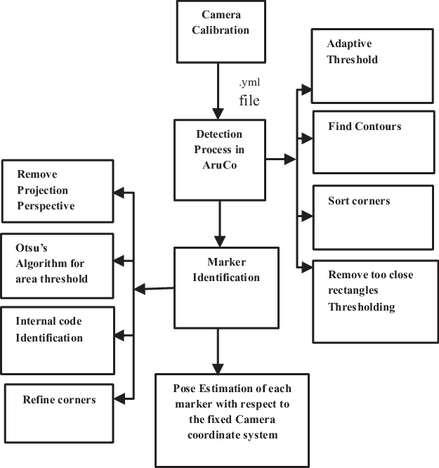
For pose estimation, the marker is placed on the target location, and the algorithm uses the entire image matrix to estimate both position and orientation with respect to the camera frame. The various steps involved in this method are camera calibration, marker detection process, marker identification, and pose estimation. The flow process is shown in Fig. 3 and is discussed in brief below.
2.2.2. Camera calibration
Camera calibration is used to estimate the intrinsic and extrinsic parameters of the camera. This is a process of characterizing parameters like focal length, principal point, skew, and image distortion. This is a one-time activity for each camera, and the quality of pose estimation is enhanced by adopting this correction process. The camera used is the Basler AG with a sensor resolution of 1280 × 960. The calibration was done using the Zhang method [Reference Zhang10], in which images from a stationary camera of a checker box positioned at the differing orientation are used. The camera calibration toolbox [Reference Bouguet18] was used to determine the intrinsic parameters via a set of 20 images. The intrinsic parameter includes focal length, principal point, skew, and distortion parameter. These intrinsic parameters determined for one of the cameras are tabulated in Table I.
Table I. Intrinsic parameter of the camera.


Figure 3. Flow diagram of marker detection in a real-time environment with respect to the fixed camera coordinate system.
2.2.3. Marker detection process
In this process, the marker placed at the target location is detected in the scene. The marker detected in the scene is given an ID number. Four different steps are followed for the detection process. The steps are adaptive thresholding, contour finding, corners detection, and rectangle thresholding. In the thresholding process, pixel intensity is set to either a foreground or background value by comparing the pixel intensity of the input image against a threshold value. In classical thresholding, this is done by comparing each pixel value to a global threshold.
This leads to below optimal results, especially in the case of varied lighting. Adaptive thresholding helps negate this problem by choosing a local threshold value over a pre-specified kernel size. Thus, mean adaptive thresholding is implemented in which the threshold value is calculated by the mean local value of the pixels [Reference Gonzalez and Woods19]. Then contour finding, corners detection, and rectangle thresholding are done. In which closed-form contours present in the binary image are detected. The coordinate of the corners present in the silhouette is determined. These coordinates are used to identify a four-sided polygon as a projection of the rectangular shape marker. Further, the contours are approximated, and only the candidates with four corners are selected as eligible, and other candidates are discarded.
2.2.4. Marker identification
For identifying the markers, the inner region of the rectangular candidate region must be analyzed. Since the marker is rarely parallel to the camera plane, the perspective correction needed is done by making the polygon sides equal and parallel to the image frame. Following this, the resultant square candidate is the other threshold to identify the inner pattern. The internal pattern of the square is divided into a grid to form cells. Once the cell is created, the binary image is decoded and compared with the markers ID available in the library. Thus, the marker is identified.
2.2.5. Pose estimation
The image of the identified marker and the marker image stored in the library is used for pose estimation. The transformation for perspective correction and damped least square method is used iteratively to minimize the projection error [Reference Kansal and Mukherjee20–Reference Basler23] and yields the pose of the marker (target position) in the camera frame. The process of determining the pose of the top platform of the 6-UScS manipulator with respect to the base platform frame is explained as follows:
The experimental setup has a top platform that is actuated to orient the cranium of the cadaver. The inertial frame is shown in Fig 2(a), where the 6-UScS manipulator has { F W } as the inertial frame. The inertial frame is aligned with the natural kinematic coordinate frame. The top platform moves with respect to the { F W }. The camera coordinate frame { F C } is fixed to the camera. The coordinate marker frame { F E } has its origin at the middle of the marker, which is determined by the ArUco algorithm shown in Fig 2(b). The ArUco marker detection algorithm (as shown in Fig. 3) is a map from the world coordinate frame [U V W] to the camera coordinate frames [X Y Z], that is, it determines the pose of the marker with respect to the camera frame as shown in Eq. (3).

Figure 4. Vector loop of the test setup for pose estimation using vision setup.
The coordinate frame {
F
M
} is attached to the platform, and the coordinate frame {
F
W
} is attached to the base platform shown in Fig. 4, having origin M
O
and O, respectively. ArUco markers are placed at points A and B having marker frame {
F
E
1
} and {
F
E
2
} with origin A
O
and B
O
, respectively. A camera frame {
F
C
} is attached to the camera with its origin C
O
. Let the vector
M
r
A
be the position vector from point M
O
to A in frame {
F
M
} and
C
r
A
the vector from point C
O
to A in the camera frame {
F
C
}. Similarly, the vector
F
r
B
is the position vector from point O to B in frame {
F
W
} and
C
r
B
is the vector from point C
O
to B in camera frame {F
C
}. Thus, the vectors
C
r
M
and
C
r
F
are known by vector addition. Let vector $\vec d$
be the vector from point O to M
O
in frame {
F
W
}. Vector
$\vec d$
be the vector from point O to M
O
in frame {
F
W
}. Vector $\vec d$
changes as the attitude of the top platform are changed. Once the vectors
C
r
M
and
C
r
F
are known, the loop closure equation can evaluate the vector
$\vec d$
changes as the attitude of the top platform are changed. Once the vectors
C
r
M
and
C
r
F
are known, the loop closure equation can evaluate the vector $\vec d$
:
$\vec d$
:
 \begin{align}^{\rm{C}}{{\bf{r}}_{\bf{f}}} + {\bf{d}}{ = ^{\rm{C}}}{{\bf{r}}_{\bf{M}}}\end{align}
The orientation of the top platform can be determined by the known rotation matrix between the coordinate frames, that is, M Q A , C Q A , C Q B , and F Q B . The equation for evaluation of M Q F (rotation matrix between the moving and fixed platform) is given by:
 \begin{align}^{\bf{M}}{{\bf{Q}}_{\bf{F}}} \,{=}\, ^{\bf{M}}{{\bf{Q}}_{\bf{A}}}^{\bf{C}}{{\bf{Q}}_{\bf{A}}^{{ - {\bf{1}}}{\bf{C}}}}{{\bf{Q}}_{\bf{B}}}^{\bf{F}}{\bf{Q}}_{\bf{B}}^{ - {\bf{1}}}\end{align}
Thus, the pose of the top platform {F W } that is, d and M Q F are evaluated. In computer vision, the relative position and orientation of an object with respect to the camera are termed as the pose. To estimate the pose of an object, we require points on the 3D object in the world frame [U V W] and the 2D points of the image [x y]. The coordinates of the 3D object in the camera frame [X Y Z] are unknown but can be calculated using the camera matrix of the 2D points. Eq. (3) describes the relationship between the object points in the world coordinate system and the camera coordinate system. The terms [ r 00 , r 01 …… r 22 ] describe the rotation matrix R while the terms [t x , t y , t z ] describe the translation vector t. The term s is an unknown scaling factor.
 \begin{align}s\left[ {XYZ} \right] = \left[ {{\textbf{r}_{\textbf{00}}}{\textbf{r}_{\textbf{01}}}{\textbf{r}_{\textbf{02}}}{\textbf{t}_\textbf{x}}{\textbf{r}_{\textbf{10}}}{\textbf{r}_{\textbf{11}}}{\textbf{r}_{\textbf{12}}}{\textbf{t}_\textbf{y}} \ldots \ldots. {\textbf{r}_{\textbf{20}}}{\textbf{r}_{\textbf{21}}}{\textbf{r}_{\textbf{22}}}{\textbf{t}_\textbf{z}}} \right]\left[ {UVW1} \right]\end{align}
 \begin{align}s\left[ {XYZ} \right] = \left[ {\textbf{r}|\textbf{t}} \right]\left[ {UVW1} \right]\end{align}
 \begin{align}\left[ {xy1} \right] = s\textbf{C}\left[ {XYZ} \right] \\[-20pt] \nonumber \end{align}
Eq. (3) describes the relationship between the camera frame 3D object points and the coordinates of the 2D points on the image plane. The term C is the intrinsic camera matrix. In the ArUco algorithm, the object points are the four corners of the marker with coordinates by the marker size. This is compared to the image points which have been detected using the camera. The image points are projected in 3D using Eq. (3), and these points are compared to the points of the object. The initial solution is obtained by solving Eq. (1) using direct linear transformation. This solution is not very accurate, so further refinement is done using the Levenberg–Marquardt Algorithm (LMA). The reprojection error is the distance between the object points and the projected image points is minimized using the LMA method. The outputs are the rotational matrix and the translational vector.
The Levenberg–Marquardt optimization function finds such a pose that minimizes the reprojection error. The reprojection error is the sum of the square distances between the observed projections and the projected object points. Thus, the method is also called the least-squares method. The function which the Levenberg-Marquardt algorithm iteratively tries to minimize is of the form:
 \begin{align}\emptyset = \sum\limits_{i = 1}^n {{{\left[ {\textbf{Y} - \hat{\textbf{Y}}} \right]}^2}} \end{align}
Where $\hat{\textbf{Y}}$
is the predicted value of
$\hat{\textbf{Y}}$
is the predicted value of $\textbf{Y}$
.
$\textbf{Y}$
.
Using the pose of the moving platform with respect to the camera and stationary base with respect to the camera, the orientation and position of the moving platform can be computed with respect to the base using
 \begin{align}^M{\textbf{H}_W} = {{[^W}{\textbf{H}_C}]^{ - 1}}^M{\textbf{H}_C}\end{align}
Where; $^M{\textbf{H}_W}:$
is the homogeneous transformation matrix of the moving platform with respect to the base.
$^M{\textbf{H}_W}:$
is the homogeneous transformation matrix of the moving platform with respect to the base. $^W{\textbf{H}_C}:$
is the homogeneous transformation matrix of the base platform with respect to the camera.
$^W{\textbf{H}_C}:$
is the homogeneous transformation matrix of the base platform with respect to the camera. $^M{\textbf{H}_C}:$
is the homogeneous transformation matrix of the moving platform with respect to the camera.
$^M{\textbf{H}_C}:$
is the homogeneous transformation matrix of the moving platform with respect to the camera.
ArUco markers are chosen instead of similar marker dictionaries such as ARTag or ARToolKitPlus because of the way markers are added to the marker dictionary. This has a direct hand during error correction while detecting markers. While creating a marker dictionary, adding markers into the dictionary is iterative and continues until a threshold is met. This depends on the Hamming distance between a marker and other markers in the dictionary and with the same marker after undergoing rotations of k times 90o, where k is 1, 2 or 3. Addition occurs till the required number of markers has been added into the dictionary. The minimum distance of a marker in a particular dictionary is $\hat \tau $
. The error correction capabilities of an ArUco dictionary are directly related to
$\hat \tau $
. The error correction capabilities of an ArUco dictionary are directly related to $\hat \tau $
. Compared to ARToolKitPlus (cannot correct bits) and ARTag (can correct up to 2 bits only), ArUco can correct up to
$\hat \tau $
. Compared to ARToolKitPlus (cannot correct bits) and ARTag (can correct up to 2 bits only), ArUco can correct up to $\left[ {\hat \tau - \frac{1}{2}} \right]$
bits. If the distance between the erroneous marker and a dictionary marker is less than or equal to
$\left[ {\hat \tau - \frac{1}{2}} \right]$
bits. If the distance between the erroneous marker and a dictionary marker is less than or equal to $\left[ {\hat \tau - \frac{1}{2}} \right]$
, the nearest marker is considered the correct marker.
$\left[ {\hat \tau - \frac{1}{2}} \right]$
, the nearest marker is considered the correct marker.
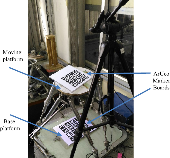
Figure 5. Experimental setup for pose estimation.
The output from the marker detection code of ArUco is the form of the position vector of the center of the marker and the Rodrigues vector of the marker frame. The Rodrigues vector is converted into a 3 × 3 rotation matrix. The following were the experimental iterations.
-
1. Single marker pose detection using translation and rotation matrix.
-
2. Three marker pose detection using only translational information from the three markers.
-
3. Pose estimation using a board with multiple evenly spaced markers.
Single marker detection revealed an almost stable translation vector but a very unstable rotation matrix. The values showed unacceptable variation for a stable platform and camera position. Even if the input is an image instead of a video stream, the rotation matrix was unreliable. Therefore, a single ArUco marker is insufficient to estimate the pose of a Stewart platform accurately. We used three ArUco markers arranged at the corners of an equilateral triangle on a side length of 10 cm. The aim was to extract plane information solely from the position vectors of the three markers. The results were more reliable than single marker detection. While moving the markers in the same plane, the plane equation derived from the pose estimation of the 3-marker system showed variation. The maximum error recorded was of the order of 5o.
A solution for unreliable pose estimation was increasing the number of markers in the form of a board and extracting the position and orientation of the board instead of individual markers. One moving this arrangement in the same place, the orientation vector of the board showed slight deviation with a maximum error of around 1o.
Kinematic analysis of the Stewart platform was attempted using marker board detection for pose estimation. A board of 16 markers, evenly spaced in the form of a 4 × 4 grid, was placed on the Base and the Platform, as shown in Fig. 5. The board for the base and platform were separate, and the markers were of different sizes. The size of the markers on the platform was of side 26.1 mm, and the markers on the base were of side length 39.4 mm. Different sizes were chosen so that the edges of the markers could be detected accurately on both the base and the platform without having to move the camera. Once the platform marker and base marker were detected with respect to the camera, as shown in Figs. 6 and 7, respectively. Using Eq. (7), estimation of the platform marker with respect to the base marker is done. The center of the boards is placed precisely on the origins of the base and the platform. Compensations for the width of the ArUco marker board were considered while calculating the position vector of the platform’s origin with respect to the base frame. The advantage of the bimodal image is that it does not affect the segmentation process inherently improve the pose estimation of the region of interest on varying the lighting condition.

Figure 6. Detected platform marker board and threshold image.

Figure 7. Detected base marker board and threshold image.
The leg lengths of the Stewart Platform were changed manually by keeping the camera stable. The resultant position and orientation of the platform with respect to the base were captured using a camera. The homogeneous transformation matrix of the platform with respect to the base is computed using the output rotation matrices and translation vectors. The leg lengths are calculated mathematically using the transformation matrix. These lengths are checked against the actual lengths of the Stewart platform, and the percentage error is calculated. This was done for 15 different configurations of the Stewart platform by manually adjusting the leg lengths. The leg lengths were changed from a minimum of 370.5 mm to a maximum of 465 mm.
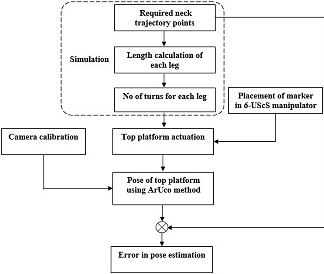
Figure 8. Flow diagram for estimating the error in the pose of the experimental setup.
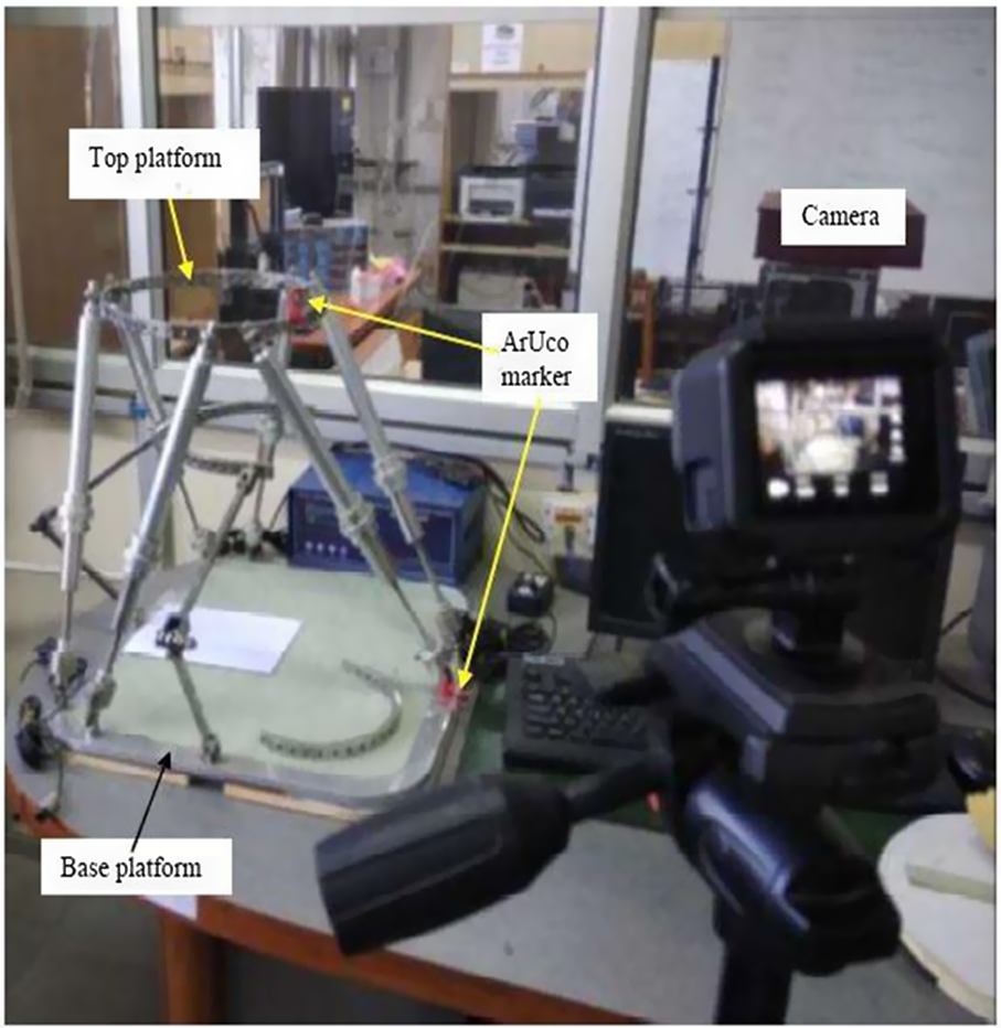
Figure 9. The layout of the experimental setup for pose estimation using single camera metrology.
3. Experiment
3.1. Pose estimation
Pose estimation of the top platform of the 6-UScS manipulator was tested out using the flowchart shown in Fig. 8. Firstly, the markers were placed on the top and base platform, as shown in Fig 9. The manipulation of the top platform was performed by actuating the screw joints. For the desired neck trajectory, that is, flexion/extension, lateral bending, and axial rotation, the number of turns required for the screw joint must be determined. The leg lengths were obtained from the inverse kinematic solution, then knowing the pitch of the screw, the number of turns was calculated. Table II shows the turn sequence required for progressive flexion motion from the top platform’s initial horizontal and centered posture. For example, the number of turns needed for the legs for flexion is −7, −9, 1, 1, 8, and 7, where a negative sign shows clockwise motion, and a positive sign shows the anti-clockwise motion of the screw.
Table II. Number of incremental turns required by the MA7DPM setup for flexion trajectory of the top platform.

During execution, this set of integer number of turns was split into sequences such that at most one turn was imparted at each screw. In this case, nine subsets were formed for flexion. The sequence provided for each cycle are (0, −1,0,0,0,0), (0, −1,0,0,1,0), (−1, −1,0,0,1,1), (−1, −1,0,0,1,1), (−1, −1,0,0,1,1), (−1, −1,0,0,1,1), (−1, −1,0,0,1,1), (−1, −1,0,0,1,1), and (−1, −1,1,1,1,1). After giving the sequential turns to the leg for achieving the desired neck trajectory, the position and orientation of the top platform were verified using Vernier caliper and bevel protractor, respectively.
Further, a Basler camera was used for vision-based pose estimation, which is specified in the Basler AG manual [Reference Kansal and Mukherjee20]. The images were taken from a calibrated camera, which was processed to evaluate the pose of the top and base platform in the camera frame {F C }. One set of such poses, quite typical of the data obtained from the camera, are tabulated in Table III. Further, using the coordinate transformation, the pose of the top platform was determined in an inertial frame {F W }. The pose obtained from the camera and the target pose data is tabulated in Table IV.
Table III. Pose of the moving and base platform estimated by the camera setup.

Table IV. Comparison of the estimated pose with that of target pose in base frame {FW}.

3.2. Observations
The absolute error ranged from a minimum of 0.1 mm to a maximum of 16 mm. The mean and median absolute errors were 3.8961 mm and 3.35 mm, respectively, while the standard deviation was 2.9878 mm. The leg lengths were altered in the range of 370.5–465 mm, as shown in Fig. 10.

Figure 10. Scatter plot of absolute error data.
3.3. Intervertebral motion estimation of the saw bone model (stability of the spine)
The spinal column plays a vital role in providing mechanical stability and housing for the spinal cord and spinal nerves. Of the total motion of the cervical spine, 25% of flexion extension and 50% of axial rotation comes from CVJ [Reference Ahmed, Traynelis and Menezes24, Reference Clark, Abdullah, Mroz and Steinmetz25]. It also protects the most critical neural and vascular structures, and thus the stability of this region is crucial. In a work by Panjabi et al. [Reference Panjabi, White and Johnson26], clinical stability is described as the ability of the spine to limit its patterns of displacement over time under physiologic loads so as not to damage or irritate the spinal cord or the nerve roots. Thus, to determine the stability of the cervical spine, intervertebral region motion study is one of the most crucial parts. This study will even help in establishing the criteria of stability of healthy CVJ and assist in defining the stability of CVJ post-implant instrumented CVJ neurosurgery (Fig. 11).

Figure 11. Scatter plot of percentage error data.
3.4. Intervertebral motion estimation of the SAW bone model
Fig. 12 shows a Manually actuated 7-DOF Parallel Manipulator (MA7DPM) consisting of a 6-UScS manipulator and Sarrus mechanism intended on a common base platform. The 6-UScS manipulator has a top and base platform connected by six legs. Load sensors are placed at the base of the leg to record the load response.

Figure 12. Detection of eight markers, that is, computing the position and rotation of each marker with respect to the fixed camera coordinate system.
The Sarrus mechanism is a 1-DOF manipulator and permits linear motion of the middle platform in the vertical direction. The middle platform is aligned along the C5 vertebra and is fastened. The customized fasteners are used to fasten the Occiput and vertebra to the top and middle platform of the MA7DPM, respectively. It consists of a poly-axial screw, coupling, and extension screw.
For the experiment, a saw bone of the cervical region was taken. The Occiput to the C7 vertebra is visible for fastening with the manipulation system. Poly-axial screws were inserted in the cranium and lateral mass of the C7 vertebrae. The C7 vertebra was attached to the middle platform by the same process. Then, ArUco markers were placed on the target location of the vertebra, as shown in Fig. 13. Finally, the camera was set up to determine the intervertebral motion based on the actuation of the manipulator.

Figure 13. Experimental setup of the intervertebral motion estimation of the Saw Bone Model (stability of the spine).
The camera setup is used to determine the pose of the top platform of the 6-UScS manipulator. Pose estimation is carried out using the ArUco method. In this method, markers were placed on top and base platforms. Once the manipulation of the top platform was performed for the desired neck trajectory, that is, flexion/extension, lateral bending, and axial rotation, the image was taken from a calibrated camera, which was processed to evaluate the pose of the top platform. Two cameras were placed, though a monocular camera determines the pose; the second camera is used as backup and verification because of the paucity of the specimen to experiment with.
3.5. Discussion
Kinematic analysis of the Stewart platform was attempted using marker board detection for pose estimation. The leg lengths of the Stewart Platform were changed manually by keeping the camera stable. The resultant position and orientation of the platform with respect to the base were captured using a camera. Table II shows the turn sequence required for progressive flexion motion from the top platform’s initial horizontal and centered posture. The absolute error ranged from a minimum of 0.1 mm to a maximum of 16 mm.
In contrast, the mean and median absolute errors were 3.8961 mm and 3.35 mm. The percentage error showed the following trends considering the absolute lengths. The percentage error was between 3.9168% and 0.0230%.
For the experiment, a saw bone of the cervical region was taken. The Occiput to the C7 vertebra is visible for fastening with the manipulation system. Poly-axial screws were inserted in the cranium and lateral mass of the C7 vertebrae. The C7 vertebra was attached to the middle platform by the same process. Then, ArUco markers were placed on the target location of the vertebra. Finally, the camera was set up to determine the intervertebral motion based on the actuation of the manipulator. Once the manipulation of the top platform was performed for the desired neck trajectory, that is, flexion/extension, lateral bending, and axial rotation, the image was taken from a calibrated camera, which was processed to evaluate the pose of the top platform.
4. Conclusion
The method of pose estimation using ArUco markers for determining the position and orientation of the platform with respect to the base reveals a mean percentage error of 0.9507%. Pose estimation using ArUco markers is, therefore, a viable method for analyzing the forward kinematics of a Stewart Platform. Increasing the size of the marker helps in edge detection. Accurate detection of edge length is to a precise position vector and rotation matrix. Increasing the number of markers on the marker board helps in providing a stable pose. Thus, this ensures a more reliable pose estimation. The pose estimation of the top platform using the single-camera metrology by the ArUco method was assessed. Incremental changes in pose induced by fixed movement of the leg were compared with the camera-based measurement to estimate pose errors.
The study of implant performance on the decapitated specimen is not necessarily the gold standard in that it removes the soft tissue effects. The work can be extended to establish methods to evaluate the implant design where; soft tissues are retained during the experiments, and the forces on the implant can be evaluated. In the future, the design and development of a setup for experimental study of the CVJ region with implants instrumented on a full cadaver can be investigated.
The performance of implants has been evaluated over the past decades by various researchers, all of which have been through the use of decapitated specimens. In the paper by Schulze [Reference Schulze, Trautwein, Vordemvenne, Raschke and Heuer1], they used the KUKA KR125 robot as the manipulator, optical motion tracking system, and X-ray images for implant performance study on a decapitated specimen. In the paper by Puttlitz [Reference Puttlitz, Melcher, Kleinstueck, Harms, Bradford and Lotz2], they used a system of weight, pulley, nylon string, and rods for applying pure couples on the human CVJ complex. Stereo-photogrammetric was used to determine the range of motion. In the paper by Goel [Reference Goel, Clark, Gallaes and Liu27], experimented on eight CVJ specimens, where the experiment was conducted by casting the C5 vertebra in a plastic padding block, and two perpendicular rods were inserted in Occiput; then, the clinical load was applied on the rods and stereo-camera were used to determine the motion.
In this article, a series of experiments have been done, and the study was conducted on a saw bone model to determine the range of motion targeted for the cadaveric investigation. The experimental setup is so designed that the decapitation of the cadaver can be avoided, and the experiment can be conducted with the intact cadaver. For conducting the experiment’s single camera and marker metrology is opted for vision-based pose estimation. The motion to the manipulator is manually actuated by changing the length of the legs (refer to Table II). Based on the pose data, the range of motion, point of motion, and intervertebral motion can be estimated. The estimated data will be used to determine the stiffness of the CVJ and determine the suitable implant [Reference Gupta, Zubair, Lalwani, Gamangatti, Shankar, Mukherjee and Kale28] for the CVJ region.
Acknowledgements
We acknowledge Mechatronics Lab, Mechanical Engineering Department, IIT Delhi, and Jai Prakash Narayan Apex Trauma Centre (JPNATC), AIIMS, New Delhi, for providing the environment for carrying out the research activity.


 Open access