


1 MOTIVATION
There has been a huge financial and personnel investment in a multitude of Milky Way stellar surveys obtaining spectra for hundreds of thousands to millions of stars. These surveys are characterised by different sky coverages, selection functions, wavelength regions, resolutions, and scientific motivations. Surveys include RAVE (Steinmetz et al. Reference Steinmetz2006), LAMOST (Newberg et al. Reference Newberg, Aoki, Ishigaki, Suda, Tsujimoto and Arimoto2012), APOGEE (Majewski et al. Reference Majewski2017), GALAH (Freeman 2012; De Silva et al. Reference De Silva2015), SEGUE (Beers et al. Reference Beers, Lee, Sivarani, Allende Prieto, Wilhelm, Re Fiorentin and Bailer-Jones2006), Gaia– eso (Gilmore et al. Reference Gilmore2012) and Gaia (Gaia Collaboration et al. 2016). Figure 1 shows an example of the complementary sky coverage of three of these ground based surveys: APOGEE, GALAH, and Gaia– eso. There are also a multitude of new surveys being planned including AS4 (Kollmeier et al., submitted), 4-MOST (de Jong et al. 2016), WEAVE (Bonifacio et al. Reference Bonifacio and Reylé2016), MOONS (Cirasuolo et al. Reference Cirasuolo, Afonso, Carollo, Flores, Maiolino, Ramsay, McLean and Takami2014) and many more.
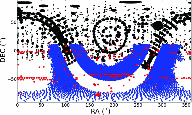
Figure 1. The complementary sky coverage of three different galactic surveys: APOGEE (in black), Gaia– eso (in red), and GALAH in blue.
These surveys are all together observing spectra for many millions of stars across the Galaxy and independently delivering stellar parameters and abundances (hereafter referred to as stellar labels) for these stars. These stellar labels themselves are intrinsic properties of the stars and thus, should be entirely independent of the spectral wavelength interval and resolution at which the data is observed. However, this is not the case, and different stellar labels are determined for the same star depending on the survey and instrument set up, wavelength, and resolution [see the Introduction of Ness et al. (Reference Ness, Hogg, Rix, Ho and Zasowski2015) and references therein]. The results obtained for a given star within a survey can also vary significantly, due to the assumptions, choices, and methodology adopted to extract the stellar labels (Jofre et al. Reference Jofre2016).
We are therefore in a situation where we have millions of spectra with labels derived from a multitude of surveys, that are all on different label scales. Thus, the data from different surveys (and across different regions of the sky) cannot be combined. There is however a solution to this problem of different scales for different surveys (and within surveys). This solution resides in the fact that for any survey, there is a small subset of stars where we know their labels with higher accuracy, precision, or both; this high fidelity set of stars with well-known labels are key reference objects. These reference objects can be cluster stars (typically used for calibration due to the external information known about these stellar populations) high signal to noise (SNR) well-studied stars including benchmark stars (i.e. Jofré et al. Reference Jofré2014) or, for example, stars for which there is external information known e.g. from asterosemisology, which is undergoing its own revolution in scale (Stello et al. Reference Stello2015). These reference objects and their labels can be used directly, to make a data-driven model and, given stars in common between surveys, this data-driven approach can be used to propagate one label scale directly from one survey to another.
The pursuit of a data-driven approach which specifically led to developing The Cannon was ultimately motivated by (1) working to solve this problem of inconsistent label scales among surveys and for data obtained at different resolutions and wavelength regions, (2) to develop a generalised approach and tool, which can be directly applied to any survey, independent of the wavelength and resolution of the data, as long as there are a set of reference objects with known labels that can be used to train a model, and (3) to understand where the information content resides in spectral data and to optimally extract this information.
2 THE ADVANTAGES OF A DATA-DRIVEN APPROACH
The data-driven approach can propagate an adopted ‘ground-truth’ of the label scale of the reference objects and is therefore accurate in as far as is the reference objects are accurate. Whilst The Cannon is data-driven, this approach ultimately relies on stellar physics and theoretical models, from which the labels for the reference objects are derived. This label scale can then be efficiently propagated within and among surveys, given stars in common between different datasets. The data-driven method has a number of advantages, which include the following:
-
(1) The Cannon is the first method that directly enables all large spectroscopic surveys (e.g. GALAH, APOGEE, Gaia– eso, LAMOST, RAVE) to be directly cross-calibrated [see Section 4.2: we have now put almost 1 million stars from different surveys on same (APOGEE) scale with this approach].
-
(2) The Cannon delivers 2–3 times smaller errors (see Section 4.1). This implies 1/4 or 1/9th observing time or more stars that can be observed for the same precision and is informing the strategy of new generation surveys (see Section 5.4).
-
(3) This has opened up new avenues in galactic archeology (e.g. higher precision for chemical tagging and stellar ages from stellar spectra) for almost a hundred thousand stars across the Milky Way disk (see Sections 4.3 and 4.4).
One powerful prospect for The Cannon and one which is yet to be exploited is that the data-driven approach can be used to inform stellar models and test stellar physics and examine directly where models diverge from data.
3 THE CANNON
The Cannon is a data-driven method to determine stellar parameters and abundances (and more generally, stellar labels) for stars in large surveys. The Cannon relies on a subset of reference stars in the survey, with known labels. These labels can come from high resolution analyses from any wavelength regions and from comparisons with the most up to date stellar models. The Cannon then uses the reference objects with known labels to build a model that relates stellar labels to stellar flux at each wavelength. That model is then used to infer the stellar labels for the remaining stars in the survey (Ness et al. Reference Ness, Hogg, Rix, Ho and Zasowski2015). The Cannon is named after Annie Jump Cannon, who pioneered producing stellar classifications without physical models. This data-driven approach is detailed in Ness et al. (Reference Ness, Hogg, Rix, Ho and Zasowski2015) and implemented in a number of subsequent papers (e.g. Ho et al. Reference Ho2016a; Casey et al. Reference Casey, Hogg, Ness, Rix, Ho and Gilmore2016a; Martell et al. Reference Martell2016). The principles and mathematics of The Cannon are detailed in Ness et al. (Reference Ness, Hogg, Rix, Ho and Zasowski2015) and I revise it only briefly here:
The Cannon relies on the following to be true in order for this approach to work: (i) stars with the same labels have the same spectra and (ii) stellar flux varies smoothly with stellar labels.
If these hold true, we use n reference objects with known labels ℓ n to build a spectral model, called Training. The spectral model is characterised by a coefficient vector θ λ that allows the prediction of the flux at every pixel f nλ for a given label vector:
 $$\begin{equation}
f_{n\lambda } = g(\bm {\ell }_n | \bm {\theta }_\lambda ) + \mbox{noise}. \quad
\end{equation}$$
$$\begin{equation}
f_{n\lambda } = g(\bm {\ell }_n | \bm {\theta }_\lambda ) + \mbox{noise}. \quad
\end{equation}$$
This relates stellar labels ℓ n to stellar flux f nλ at each wavelength. The noise is an rms combination of the associated uncertainty variance σ2 nλ of each of the pixels of the flux from finite photon counts and instrumental effects and the intrinsic variance or scatter of the model at each wavelength of the fit, s 2 λ.
This model is then used to infer the remaining stars in the survey, in the Test step.
In the simplest case, the training step can be done with three labels ℓ = Teff, log g, [Fe/H]. In the simplest functional form that can be subsequently assumed, equation (1) can then be written as a linear function of the vector ℓ n built from the labels:
 $$\begin{equation}
f_{n\lambda } = {a_\lambda } + {b_\lambda } (\mbox{$\rm T_{eff})$}_n + {c_\lambda } \mbox{$\rm (\log g)$}_n + {d_\lambda } \mbox{$\rm ([Fe/H])$}_n + \mbox{noise}. \quad
\end{equation}$$
$$\begin{equation}
f_{n\lambda } = {a_\lambda } + {b_\lambda } (\mbox{$\rm T_{eff})$}_n + {c_\lambda } \mbox{$\rm (\log g)$}_n + {d_\lambda } \mbox{$\rm ([Fe/H])$}_n + \mbox{noise}. \quad
\end{equation}$$
At training time, the coefficient vector is solved for (at every wavelength). In the functional form of equation (2), it is the θλ = a λ, b λ, c λ, d λ that are determined as well as the scatter, s 2 λ in the noise term.
Then at test time, using these coefficients solved for at training time, the same equation is used, only now solving for the labels of the m reference objects, labels l m = (Teff, log g, [Fe/H]) m , given their stellar flux f mλ.
 $$\begin{equation}
f_{m\lambda } = a_\lambda + b_\lambda { \mbox{($\rm T_{eff})$}}_m + c_\lambda {\mbox{$(\rm \log g)$}}_m + d_\lambda ({ \mbox{$\rm [Fe/H])$}}_m + \mbox{noise}. \quad
\end{equation}$$
$$\begin{equation}
f_{m\lambda } = a_\lambda + b_\lambda { \mbox{($\rm T_{eff})$}}_m + c_\lambda {\mbox{$(\rm \log g)$}}_m + d_\lambda ({ \mbox{$\rm [Fe/H])$}}_m + \mbox{noise}. \quad
\end{equation}$$
In practice, the simplest linear form is insufficient to describe the change of flux with stellar labels. Instead, we found the quadratic form to be extremely effective, which simply increases the model complexity to include the squared terms and cross terms of the labels, so in the case of three labels, the coefficient vector is comprised of 10 terms, rather than 4 in the linear example above.
3.1. The APOGEE example
The Cannon was developed using the APOGEE spectra, which has now observed almost 300 000 primarily red giant stars (the DR14 release). Specifically, The Cannon was first developed however on the APOGEE DR10 data release, using the ≈50 000 publicly available reduced and velocity shifted red giant stellar spectra and the corresponding DR10 labels determined by APOGEE’s aspcap pipeline (Holtzman et al. Reference Holtzman2015). The reference objects comprising the training set used to develop and test The Cannon were 540 open and globular cluster stars, with their training labels from aspcap apogee’s pipeline, as shown in Figure 2 in the Teff−log g plane. The only amendment to the spectra itself that was provided by APOGEE was to implement our own (SNR independent) continuum normalisation, described in Ness et al. (Reference Ness, Hogg, Rix, Ho and Zasowski2015). We used the APOGEE survey to develop this technique on as the reduced spectra and stellar parameters were publicly available and documented. However, The Cannon can and has been demonstrated to work at the same high precision for numerous other surveys, including across different wavelength regions, e.g. the optical region for the GALAH survey (Martell et al. Reference Martell2016) and at low resolution, e.g. for RAVE (Casey et al. Reference Casey2016b) and LAMOST (Ho et al. Reference Ho2017a,Reference Ho, Rix, Ness, Hogg, Liu and Ting2017b)]. Furthermore, Ting et al. (Reference Ting, Rix, Conroy, Ho and Lin2017) have recently demonstrated that it is possible to measure a multitude of precision abundances (14 elements at a precision of < 0.1 dex) even at a resolution of R = 1800 from LAMOST spectra using a data-driven modeling approach.
Figure 2. The 540 open and globular cluster stars used in the training set for the initial development and test of The Cannon, shown in the Teff−log g plane with corresponding Padova isochrones of the cluster age and [Fe/H]. From Ness et al. (Reference Ness, Hogg, Rix, Ho and Zasowski2015).
The training set of 540 open and globular cluster stars worked very effectively and returned very precise Teff, log g, and [Fe/H] labels for the remaining 50 000 APOGEE red giant spectra at test time, as detailed in Ness et al. (Reference Ness, Hogg, Rix, Ho and Zasowski2015). The label space of the main sequence of the training set was extremely restricted (to a single metallicity of the Pleiades cluster with main sequence objects), hence our high-fidelity labels returned were for the red giant stars only, where the training set spanned the giant branch across –2.5 > [Fe/H] > 0.5. However, main sequence stars separated into the correct parameter space at test time along the Teff−log g plane due to the inclusion of this small set of main sequence training stars (from the Pleiades). For the red giant stars at test time, the generated model from The Cannon’s best fit parameters matches the data extremely well and The Cannon uses full spectrum and error-weighted information in each pixel (Figure 3) and returns the stellar labels to very high precision (see Figure 4 for the example of the precision measured for the [Fe/H] label as a function of SNR).
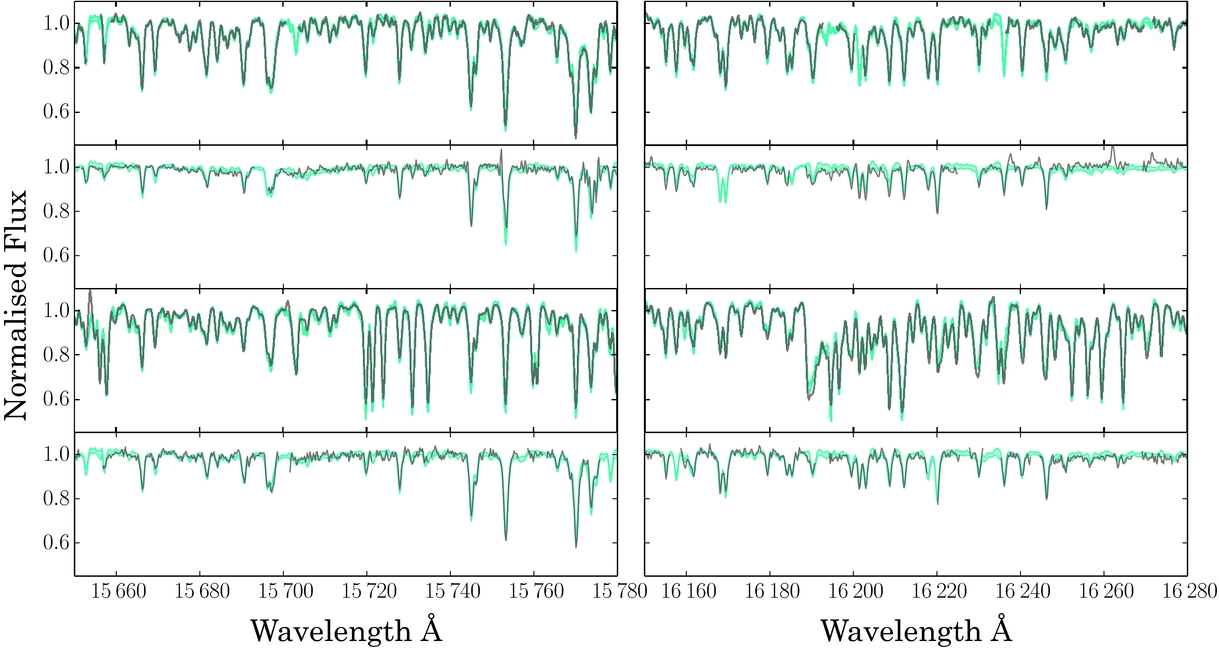
Figure 3. The data in black and the generated model from The Cannon in cyan for four example APOGEE stars (not in the training set), showing two narrow regions of the H-band spectrum for each star. These figures demonstrate that The Cannon very well reproduces the data, even with only three stellar labels of Teff, log g, and [Fe/H] used to describe the stellar spectra. From Ness et al. (Reference Ness, Hogg, Rix, Ho and Zasowski2015).
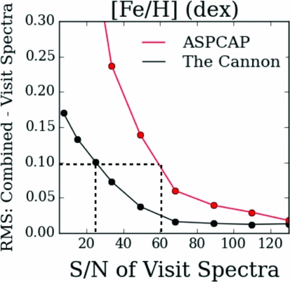
Figure 4. The precision in the [Fe/H] label of The Cannon as a function of SNR, compared to the traditional approach to determining stellar parameters and abundances (i.e. aspcap, which is representative of the best current performance obtained by the multitude of surveys). These stars comprise a set for which multiple observations (or visits) have been taken, so the rms difference can be determined based on The Cannon’s and aspcap’s results for the combined versus the individual visit spectra.
The coefficients that are returned for each label [i.e. the quadratic form of equation (3)] reveal where the information resides in the data: where a given coefficient is near zero, there is a negligible change in the flux at that wavelength for the label(s) that correspond to that coefficient. Where the coefficient value is high (either positive or negative), the flux is sensitive to that particular corresponding label at that wavelength. An example of this is shown in Figure 5. This Figure shows at the top panel the zeroth coefficient, which is approximately the median spectra of the training stars and a number of lines are marked. The middle panel shows the leading coefficients for The Cannon’s model, in this case, from the model from Ness et al. (Reference Ness, Hogg, Rix, Martig, Pinsonneault and Ho2016b), where each leading coefficient is normalised to its maximum absolute value. The bottom panel shows a generated spectra where all labels in the model are fixed except for the log g. The wavelength regions shown in this figure are centred around the two highest log g leading coefficients and demonstrate that the wings of a Mg i line and the Brackett feature are the most log g sensitive regions in the APOGEE spectra. This matches the expectations from already established stellar physics and demonstrates that the coefficients themselves carry the information as to where the most information rich regions of spectra are. Additionally, the coefficients can also be used to find and identify new atomic lines in poorly characterised regions of spectra (see Figure 19).
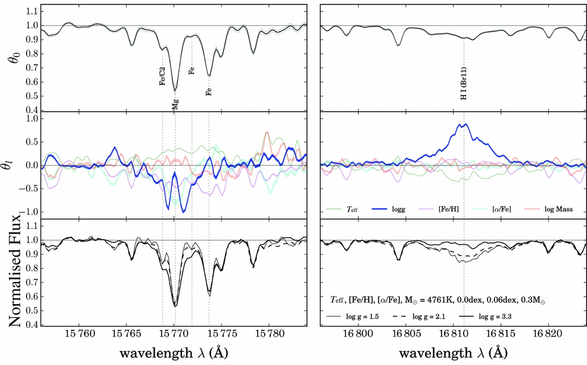
Figure 5. Top panel: normalised flux centred around the most log g sensitive features in the APOGEE spectral region as indicated by the highest two (absolute) values of the leading coefficient corresponding to the log g label. Middle panel: the leading coefficients for The Cannon’s model in Ness et al. (Reference Ness, Hogg, Rix, Martig, Pinsonneault and Ho2016b), normalised to the maximum absolute value of each coefficient. Bottom panel: the generated spectra from The Cannon’s model showing the regions with all labels fixed except the log g, demonstrating how the spectra change with varying log g. From Ness et al. (Reference Ness, Hogg, Rix, Martig, Pinsonneault and Ho2016b).
4 APPLICATIONS
The Cannon is a generative model and tool which enables the optimal exploitation of the information content of data and can identify where the most information rich regions of the data are. The Cannon has so far been developed on and applied to stellar spectra, where a simple quadratic model is sufficient to describe the way that stellar flux changes with stellar labels. The following section outlines some of the many directions this new and powerful approach is enabling, where stars are used as the tools to understand Milky Way formation.
Note that there are numerous additional applications of this approach and The Cannon’s very high precision performance at low SNR (i.e. Figure 4) means this is an ideal tool to apply to faint populations of the Milky Way or to galaxy spectral data.
4.1. Precision individual abundances
The Cannon exploits the full information in the spectrum, at all pixels, resulting in uncertainties that are 2–3 times smaller than current approaches. (Or, with this approach, we can get the same precision at 4–9 times shorter exposures). This is demonstrated in Figure 6, which shows the performance of The Cannon compared to APOGEE’s pipeline aspcap for the stellar parameters of Teff, logg, [Fe/H], [α/Fe]. Additionally, in contrast to current approaches, The Cannon is computationally very fast. The entire APOGEE dr13 150 000 star survey can be processed (returning stellar parameters) in a few hours on a single computer (Ness et al. Reference Ness, Hogg, Rix, Ho and Zasowski2015).

Figure 6. The higher precision of the stellar parameters determined by The Cannon (in black), as compared to APOGEE’s pipeline aspcap (in red) (García Pérez et al. Reference García Pérez2015). The rms difference for Teff, logg, [Fe/H], [α/Fe] is measured by comparing the labels returned for high SNR combined visit spectra to that of the lower SNR of individual visits.
The Cannon can be trivially expanded beyond stellar parameters and can be trained on individual abundances, simply by adding additional labels and solving for their corresponding coefficients using the same quadratic model. This has been done for a number of surveys. For APOGEE spectra, we have released 15 precision abundances for 90 000 red giant stars (Casey et al. Reference Casey, Hogg, Ness, Rix, Ho and Gilmore2016a) and 20 precision abundances for the open cluster stars with additional corrections that account for variations in the line spread function as a function of fibre number (Ness et al. Reference Ness2017). The individual abundances delivered with The Cannon are also being delivered at much higher precision, at a lower SNR, than is currently being achieved. Figure 7 shows a sample of our abundance precisions determined with The Cannon compared to the current performance, as demonstrated using the example of the aspcap results.
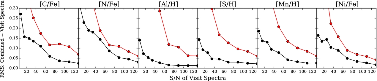
Figure 7. The same as Figure 6 and for the same set of calibration stars, but showing the performance of The Cannon and APOGEE’s pipeline aspcap for a sample of individual elements. With The Cannon, we can achieve an individual abundance precision on most elements of <0.1 dex at SNR of 50 and <0.05 dex at SNR of 80.
The Cannon (+SME) is the pipeline that is being used to deliver abundances for the GALAH survey (Martell et al. Reference Martell2016, Buder et al. in preparation) and also the upcoming 4-MOST and MOONS surveys. Such high precision abundances are critical for chemical tagging prospects (see Section 4.4). High precision enables groups of stars to be identified using their abundance information (see Figure 8) and Figure 9 shows how scientific analyses can be effectively performed using lower SNR data than previously. Almost all APOGEE stars are observed at an SNR > 100 where the analyses of Nidever et al. (Reference Nidever2014) and Hayden et al. (Reference Hayden2015) demonstrated that low-alpha sequence of stars is concentrated to the outer region of the Milky Way and the high-alpha sequence of stars to the inner. This result can be seen at much lower SNR for the results from The Cannon (i.e. Figure 9).
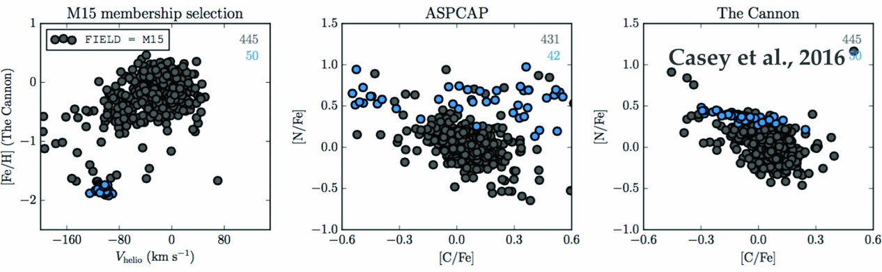
Figure 8. At left, the APOGEE field containing M15 members which can be identified from their [Fe/H]–V helio and indicated as blue circles, other field stars are shown in grey. At centre and right, the [C/Fe] vs. [N/Fe] obtained from aspcap and The Cannon, again with the cluster members in blue and stars along the line of sight in grey, this shows that the high precision results from The Cannon form a tight sequence for the cluster stars in the [C/Fe] vs. [N/Fe] abundance measurements. From Casey et al. (Reference Casey, Hogg, Ness, Rix, Ho and Gilmore2016a).
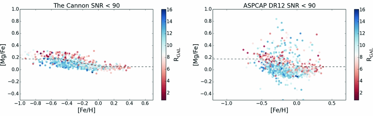
Figure 9. The [Fe/H] vs. [Mg/Fe] coloured by RGAL for the same set of SNR < 90 stars from the red clump sample in APOGEE (Bovy et al. Reference Bovy2014) at left with The Cannon’s results and at right with aspcap’s results. The low-alpha sequence of stars is concentrated to the outer region of the Milky Way and the high-alpha sequence of stars to the inner region, as first shown from high SNR data (SNR > 150) in Nidever et al. (Reference Nidever2014) and Hayden et al. (Reference Hayden2015). This is apparent in the low SNR data for the high precision results from The Cannon at left, but this is far less clear from the aspcap results at right.
4.2. Putting all surveys on a common scale
The power of the data-driven approach of The Cannon is that surveys can be placed directly on the same scale, using stars in common between the surveys. The procedure to do this is as follows: (i) there must exist stars in common between the two surveys at different (R, λ), (ii) using these stars in common, take the high fidelity labels from survey A and make the model using spectra from survey B, and (iii) apply this model made using survey A labels and survey B spectra to the remaining stars in survey B: survey B is then directly on survey A label scale.
With The Cannon, we have delivered a catalogue of high precision stellar parameter and individual abundance labels not only for the public data release of APOGEE, for 150 000 red giant stars (Casey et al. Reference Casey, Hogg, Ness, Rix, Ho and Gilmore2016a; Ness et al. Reference Ness, Hogg, Rix, Martig, Pinsonneault and Ho2016b), but also for LAMOST for 450 000 red giant stars (Ho et al. Reference Ho2016a, Reference Ho2017) (see Figure 10) and for RAVE for 500 000 stars (Casey et al. Reference Casey2016b) (see Figure 11), using the procedure described above. The red giants in APOGEE, LAMOST, and RAVE have therefore all been placed on the same (APOGEE) stellar label scale. Thus, we now have almost a million stellar spectra covering the spatial extent of the Southern and Northern sky, directly on the same label scale: this data can be used as a single powerful set for scientific analyses. There is the opportunity to also do this for 300 000 SEGUE stars as well as put GALAH (which has currently observed 300 000 stars with the aim to observe 1 million stars) and APOGEE (which has currently observed 300 000 stars with the aim to observe 450 000 stars) on a common scale using the > 1 000 stars in common between these surveys. Future surveys should cooperate to ensure common reference stars are observed, in which case these future surveys can be placed directly on the same label scale with a data-driven methodology like The Cannon.
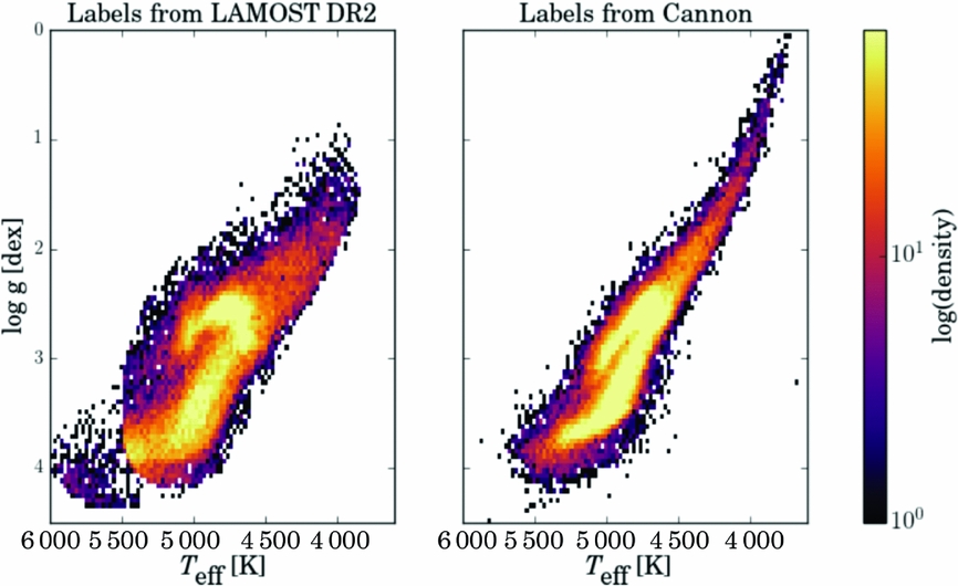
Figure 10. The Teff−log g plane of 450 000 LAMOST red giant stars showing the results from the LAMOST pipeline at left and from The Cannon’s results at right (on the APOGEE scale), derived using a model built from 10 000 stars in common between APOGEE and LAMOST (Ho et al. Reference Ho2016a).
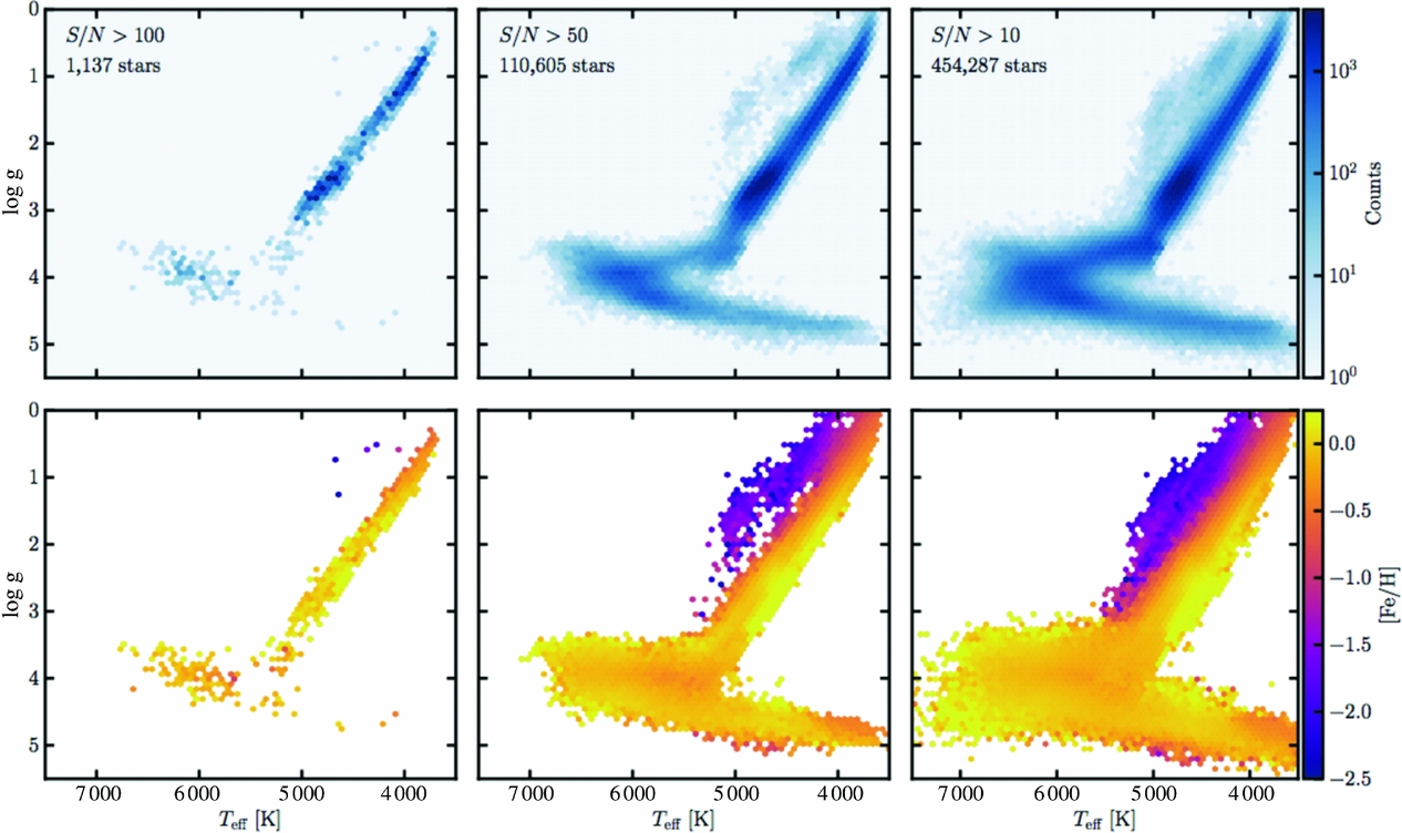
Figure 11. The Teff−log g plane of the RAVE stars that have been placed on the APOGEE label scale (for the red giants) broken up into three panels, as a function of SNR and showing stellar density at top and coloured by [Fe/H] at bottom. From Casey et al. (Reference Casey, Hogg, Ness, Rix, Ho and Gilmore2016a).
4.3. Stellar mass from stellar spectra
Stellar mass is a fundamental parameter that has been difficult to derive directly from stellar spectra for red giant stars, the bright tracers that span across large spatial extents of the Milky Way. There now exists however a set of several thousand red giant stars, observed by both the Kepler mission and APOGEE survey, with high-quality spectra and asteroseismic masses, the so-called apokasc sample (Pinsonneault et al. Reference Pinsonneault2014). We can use these extremely valuable stars as reference objects, with their known stellar masses from asteroseismology and inferred ages from these masses, to build a data-driven spectral model using The Cannon. Their stellar parameters of Teff, logg, [Fe/H], [α/Fe] have been determined from the APOGEE pipeline, aspcap, and the stellar mass has been determined from their asteroseismic labels (e.g. Kjeldsen and Bedding Reference Kjeldsen and Bedding1995).
The Cannon’s model learns how changing stellar mass affects the stellar spectra, thus we can derive stellar masses from red giant spectra via this mathematical approach. Given stellar mass for a red giant star, we can infer a stellar age using the stellar evolution models. Inferred ages are arguably the fundamental variable for studying galaxy formation and evolution, given that galaxy formation is itself, quite simply, a temporal process.
The model for The Cannon, built from these valuable reference objects, with their five labels of Teff, logg, [Fe/H], [α/Fe], and mass, can determine stellar masses to ~0.07 dex from APOGEE dr12 spectra of red giants, these imply age estimates (determined from their masses using interpolation between the isochrones), accurate to ~0.2 dex (40%). This is described in detail in Ness et al. (Reference Ness, Hogg, Rix, Martig, Pinsonneault and Ho2016b). Figure 12 shows The Cannon’s performance. The top panels show the cross validation results comparing the input (aspcap) and output (The Cannon) labels and the bottom panels show the histograms of the Δ(input−output) for each label.
Figure 12. Cross validation of the training dataset of 1 639 apokasc stars observed by both APOGEE and Kepler for the Teff, logg, [Fe/H], [α/Fe], and mass labels: the results for The Cannon’s labels for training performed on 90% of the stars, showing the performance at test time on the 10% of the stars not included in training, run 10 times. The panel on the far right is the derived age label from the mass determined with The Cannon, using interpolation with PARSEC isochrones. From Ness et al. (Reference Ness, Hogg, Rix, Martig, Pinsonneault and Ho2016b).
We have delivered a catalogue of age labels for 70 000 red giant stars from APOGEE’s dr12 data release in Ness et al. (Reference Ness, Hogg, Rix, Martig, Pinsonneault and Ho2016b) that span from the galactic centre out to RGAL = 20 kpc. For APOGEE spectra, The Cannon constrains these ages from spectral regions with CN absorption lines, elements whose surface abundances reflect mass-dependent dredge up (Ness et al. Reference Ness, Hogg, Rix, Martig, Pinsonneault and Ho2016b; Martig et al. Reference Martig2016). Using The Cannon, we are able to learn directly how these blended absorption features are related to change in stellar mass. We have determined that the age information in the spectra is not a corollary of the birth-material abundances [Fe/H] and [α/Fe] and that within a mono-abundance population of stars, there are age variations that vary sensibly with Galactic position (see Figure 13).
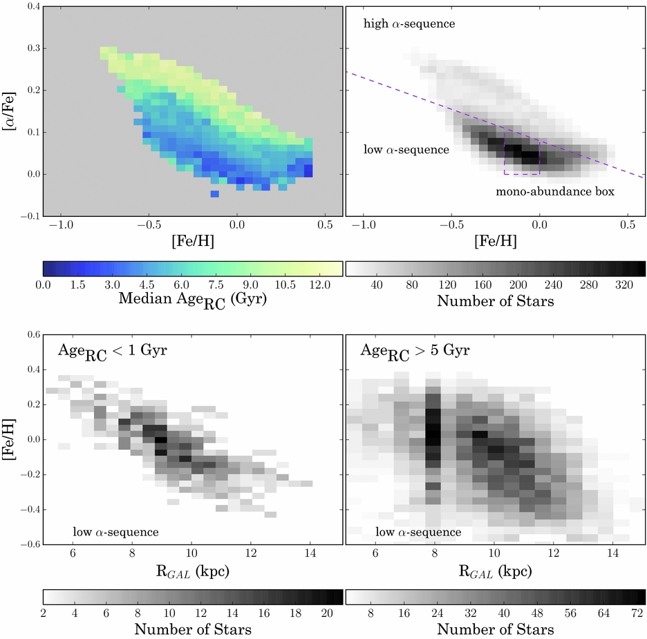
Figure 13. The 17 065 red clump stars in APOGEE (Bovy et al. Reference Bovy2014). The top left panel shows all stars coloured by median age. The density distribution of this sample is shown at the top right and the sequences we use for examining the age of the disk, of the low-α sequence and mono-abundance population bins are indicated. The bottom panels show the [Fe/H]–RGAL distribution for the young and intermediate age stars, in the low-α sequence. These bottom panels show the effect of radial migration in the Galactic disk, that [Fe/H] is a good predictor of radius for young stars in the disk, but, under the prediction of radial migration, at any given [Fe/H] older stars will be more dispersed in radius, exactly what is seen in these figures. From Ness et al. (Reference Ness2016a).
The age map that has been derived for the 70 000 red giant stars in APOGEE survey is shown in Figure 14. This is the first global age map of the Milky Way, and represents an extremely important and new avenue opened up by The Cannon in deriving stellar mass and therefore inferred age from stellar spectra, for red giant stars which can be observed to large distances across the Galaxy. The oldest stars are concentrated to the Galactic centre and youngest stars to the outer Galaxy, which is evidence of inside-out formation of the Milky Way disk.
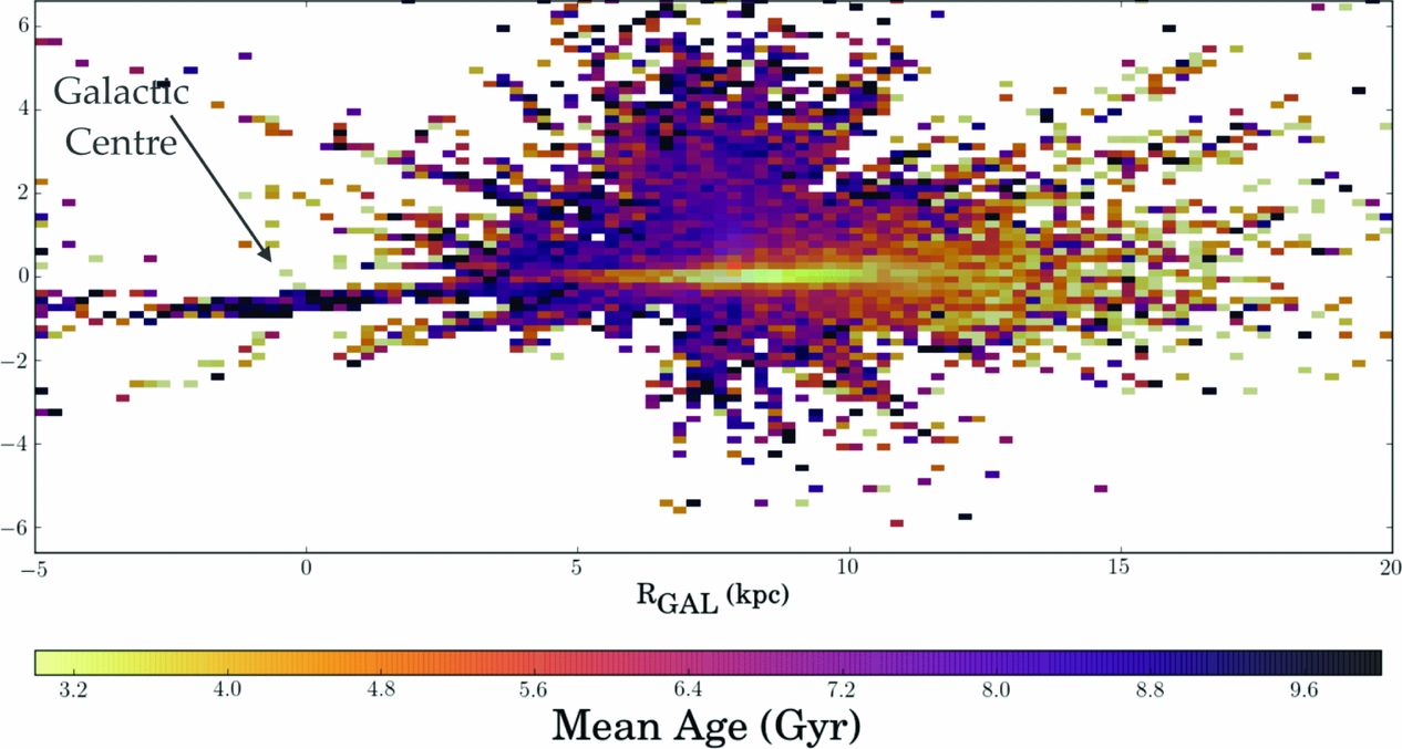
Figure 14. The age map for the Milky Way from 70 000 red giant stars binned across RGAL-z and coloured by mean age, from Ness et al. (Reference Ness, Hogg, Rix, Martig, Pinsonneault and Ho2016b). Young stars are concentrated to the plane, older stars are concentrated above the plane and to the inner region of the Galaxy. This map is evidence for inside-out formation of the Milky Way. Note also the apparent flaring of young stars which appear at larger heights from the plane at larger RGAL.
Using 10 000 red giant stars in common between APOGEE and LAMOST, Ho et al. (Reference Ho, Rix, Ness, Hogg, Liu and Ting2016b) built a model from the APOGEE labels using the LAMOST spectra to derive C and N abundances for 250 000 red giant LAMOST stars (and therefore directly on the APOGEE scale). Using the C and N abundances, a stellar age can be inferred using the relation of Martig et al. (Reference Martig2016), determined using the apokasc sample. The combined age map from APOGEE and LAMOST is shown in Figure 15. This map contains a total of over 300 000 red giant stars and demonstrates the detailed age gradients across the Galaxy as a function of (l, b), from young stars in the plane to old stars in the Galactic halo.
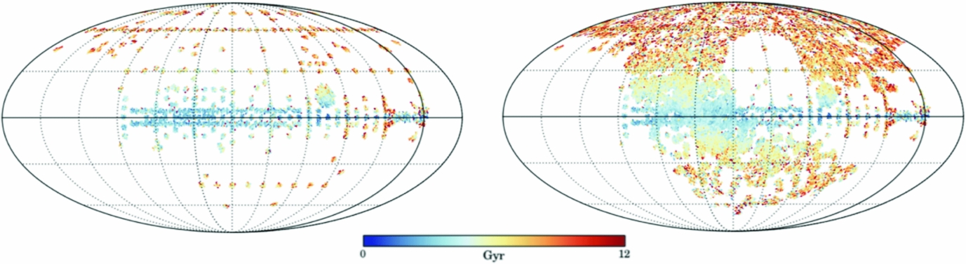
Figure 15. Aitoff on sky projection of 70 000 APOGEE red giant stars ages from Ness et al. (Reference Ness2016a), at left and for 250 000 LAMOST red giants (Ho et al. Reference Ho, Rix, Ness, Hogg, Liu and Ting2016b) and the 70 000 APOGEE red giants, at right. The ages for the LAMOST stars were determined by Ho et al. (Reference Ho, Rix, Ness, Hogg, Liu and Ting2016b) using the C and N abundances derived from the LAMOST spectra using The Cannon and are on the APOGEE label scale. The gradients in age projected on the sky are clear, with younger stars in the plane and the oldest stars in the stellar halo. The oldest stars are not seen in the Galactic centre similarity to Figure 14 simply as this projection integrates along the line of sight and the majority of the stars are only a few kpc from the Sun, the median age of these nearby stars in the disk including towards the galactic centre, is relatively young. Figure from Ho et al. (Reference Ho, Rix, Ness, Hogg, Liu and Ting2017b).
4.4. Precision abundances for chemical tagging
The Milky Way affords an ultimate test of Galaxy formation, it is a typical spiral galaxy with the majority of mass residing in the disk (~75%) and bulge (~24%). We are in the unique position to resolve individual stars in the Milky Way and derive a powerful set of measurements from those stars. These measurements include stellar age, mass, chemical compositions, and orbits which essentially represent the best set of observational quantities we can hope to measure. The quantities of stellar age, mass, and chemical compositions can be determined using stellar spectra themselves and stellar orbits can be inferred from satellite mission data, which measures the movement of stars over many epochs, most notably, the Gaia mission.
Early and turbulent formation and subsequent evolution (like radial migration and mixing) erase much of the dynamical information that would be useful for the task of reconstructing the formation and subsequent evolution of the Milky Way and particularly, of the enrichment history of the Milky Way disk, where the majority of the mass resides. Chemical compositions, however, are birth properties of stars and this is the (powerful set of) information that we have to work towards this task, of piecing together how our galaxy has formed and evolved.
There are different approaches that can be employed to use the chemical composition measurements of stars to reconstruct the enrichment history of the disk. One of these is chemical tagging (Freeman and Bland-Hawthorn Reference Freeman and Bland-Hawthorn2002). This is premised upon the Milky Way disk being made up of building blocks of now dispersed star clusters, which are stars that are born together, formed from the same gas. The expectation is that the stars from the same cluster have identical or near identical chemical compositions (Bland-Hawthorn, Krumholz, and Freeman Reference Bland-Hawthorn, Krumholz and Freeman2010). These stars clusters disperse in the turbulent disk forming and subsequent evolutionary processes like radial migration and mixing.
Chemical tagging is a discrete approach, of reconstructing the initial disk assembly and chemical enrichment history by identifying now spatially and dynamically disconnected stars that originate from the same birth sites using their chemical compositions. Conversely, one could take a probabilistic approach of describing the distribution of stars in the disk in order to trace back disk assembly and enrichment. That is, map and quantify the overall distribution of observed (precision abundances, ages, R, z, orbits) for hundreds of thousands to millions of stars in the Milky Way disk so as to measure, for example, the relative properties of stars (both spatial and orbital) that are most chemically similar to those that are least chemically similar. A probabilistic approach aimed at looking at the full distribution of observables exploits all of the information available, but intrinsically poses a less well-defined question and problem to solve compared to that of chemical tagging.
The high precision results from The Cannon for APOGEE red giant spectra, for 15 individual abundances, have been used to demonstrate that stellar phase–space structures can be identified, purely by their chemical-abundance similarity (Hogg et al. Reference Hogg2016). This is the premise of chemical tagging. This implementation in Hogg et al. (Reference Hogg2016) used a simple k-means clustering algorithm on the 15 precision abundances determined with The Cannon for 90 000 APOGEE red giant stars and recovered known phase space clusters, including M13 as shown in Figure 16. Figure 17 shows the M13 stars recovered, from Figure 16, in a two-dimensional projection in abundance space, highlighting that these group in the lower (2D) dimensionality abundance space. However, this also highlights that these (globular cluster) stars are far removed from the main population of the Milky Way disk: so while chemical tagging can work, in that phase–space structures can be recovered purely by their chemical-abundance similarity, it is working in the regime of outliers from the main distribution. That is, this works to recover the metal-poor globular clusters in the stellar halo.
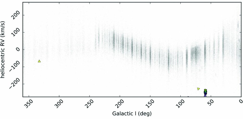
Figure 16. The 90 000 red giant stars in APOGEE’s DR12 data release shown in grey and the M13 globular cluster stars recovered using the k-means clustering algorithm shown in coloured symbols, these cluster stars are grouped in the Galactic longitude-heliocentric radial velocity plane. From Hogg et al. (Reference Hogg2016).
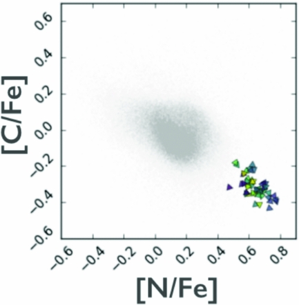
Figure 17. The [N/Fe] vs. [C/Fe] determined using The Cannon for the M13 stars shown as symbols as per Figure 16 and for the 90 000 red giant stars from APOGEE’s DR12 data release in grey, all with stellar abundances derived from The Cannon. The stars in M13 cluster in two-dimensional abundance projections, as per the example above showing [C/Fe] vs. [N/Fe]. From Hogg et al. (Reference Hogg2016).
To reconstruct the assembly of the disk with chemical tagging, we need to specifically ask if the approach of grouping stars using their chemical similarity to one another can work for the stars that comprise the disk. That is, those stars in the median of the distribution of the high-dimensional abundance space (the grey points in Figure 17). To answer this question, we examine the chemical similarity of stars that are known members of open clusters: the dissolved components of which are thought to be the building blocks of the Milky Way disk. Known open clusters (that are still spatially coherent) set the expectation for how chemically similar true birth siblings are to one another. Specifically, we use ≈ 100 stars in seven open clusters targeted by APOGEE in order to examine how chemically similar pairs of stars that are known to be born together are so called intra-cluster pairs. We contrast this with the similarity of random pairs of field stars in the disk. Our results, from Ness et al. (Reference Ness2017), are summarised in Figure 18.
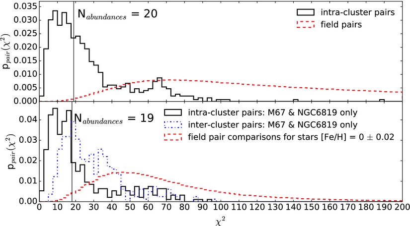
Figure 18. At top, the χ2 distribution in 20-element abundance space of all intra-cluster pairs (black) and field pairs of stars (red). This shows that typically cluster stars are identical in their 20-element abundances, within the errors, with some exceptions and stars in the field are more dissimilar from one another than stars within a given cluster. At bottom, restricting the comparison to stars [Fe/H] = 0 ± 0.02, two clusters at solar metallicity are used for the intra-cluster pairs (in black) and the inter-cluster pair similarity between these two clusters is also shown, in blue. Similarly, to the top panel, the stars within a cluster are far more chemically similar than field stars at the same [Fe/H]. Nevertheless, there is a non-negligible fraction of stars from the field (restricted to [Fe/H] = 0 ± 0.02) that are as similar to each other as stars that are from the same birth cloud, that is, the open cluster stars. These (unrelated) field stars that are as chemically similar as open cluster stars are doppelganger. From Ness et al. (Reference Ness2017).
Figure 18 shows, via a χ2 comparison of pairs of stars in 20-element abundance space using precision abundances measured with The Cannon and carefully assessed associated errors, that most stars within a cluster have abundances in most elements that are indistinguishable from those of the other members, as expected for stellar birth siblings. This figure also shows that there are highly significant abundance differences for the vast majority of field pairs and that the APOGEE-based abundance measurements have high discriminating power. The top panel shows pair comparisons across all metallicities and the bottom panel is restricted to a single metallicity (to first order, stars that are from the same birth cluster must have the same metallicity).
However, what is key to this result is that pairs of field stars whose abundances are indistinguishable (even at our high precision which is of the order of ~0.03 dex) exist—and are not very rare. What we find, is that for stars with a metallicity of [Fe/H] = 0 ± 0.02 (the bottom panel of Figure 18), that 1.0% of field pairs have χ2 differences as small as the median χ2 among intra-cluster pairs: these stars are doppelganger. That is, they are as chemically similar as the stars that are born together, from known open clusters, but are not from the same birth sites (note these doppelganger field pairs are separated by many kpc in the disk).
This high doppelganger occurrence is fatal to the viability of chemical tagging. Optimistically, the cluster mass is, at most ≈1 × 10⁶ M⊙, and the disk mass ≈1 × 10¹⁰ M⊙. Therefore, we expect 1 in 10 000 random pairs to be true birth siblings (which means that for a given random star, there is a probability that another randomly chosen star is a birth sibling of 1 × 10⁻⁴). What we find however, is that 1 in 100 field pairs are as similar as birth siblings, yet are not related these stars are doppelganger (this is a rate of 1 × 10⁻², which is far dominant over rate of true birth pairs). The conclusion is therefore that chemical tagging will not work with data of this quality and precision. However, what this analysis shows is that there is a huge amount of information for probabilistic chemo-orbital modelling (and note, that 99% of field stars are more dissimilar than open cluster stars).
5 FUTURE DIRECTIONS
5.1. Where the information in the spectral data resides
Using the regularised version of The Cannon, which sets small values of The Cannon's coefficients on the labels to zero, described in Casey et al. (Reference Casey, Hogg, Ness, Rix, Ho and Gilmore2016a), new lines corresponding to individual elements can be clearly identified using The Cannon’s first-order coefficients. The example shown in Figure 19 illustrates the first-order coefficient from The Cannon’s model for the [Al/H] label (at bottom), cross matched with the available line list (indicated at top), showing that two of the three regions of flux dependence of the label are known Al lines and the third region where the coefficient has a high value is a newly identified Al line in the spectra, that was not initially included in the DR10 linelist.
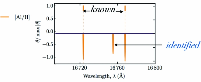
Figure 19. From Casey et al. (Reference Casey, Hogg, Ness, Rix, Ho and Gilmore2016a) showing the location of known Al absorption lines in the spectra (at top) and the Al coefficient at bottom, for the regularlised version of The Cannon which demonstrates the identification of a new Al line in the spectra, The Cannon has learned from the quadratic model where stellar flux changes with the Al label.
As another example, now in the optical spectral region, the first-order coefficient corresponding to the log g label has been examined in the GALAH spectra, to test regions of highest log g sensitivity. Figure 20 shows, at top, the first order log g coefficient and at bottom 100 random GALAH spectra. The large value of the log g coefficient corresponds to the centre of an Sc ii line. This Sc ii line is log g-sensitive because it is ionised and therefore is sensitive to pressure (and gravity) following Saha’s ionisation equation. Together with Sc i lines, this feature is typically used for estimating surface gravity under the constraint that the star must be in ionisation equilibrium. Although this estimation is performed most commonly using Fe i and Fe ii lines under the assumption of equilibrium in spectroscopic studies, the addition of Ti i/Ti ii, and Sc i/Sc ii provides additional information which increases the precision of the log g measurement. Thus, The Cannon’s results match expectations from stellar physics and conversely, can be exploited to inform stellar physics.
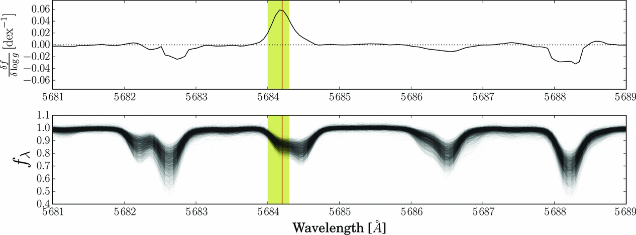
Figure 20. At top, the first-order log g coefficient and at bottom 100 random GALAH spectra. The large value of the log g coefficient corresponds to the centre of an Sc ii line. This Sc ii line is log g-sensitive because it is ionised and therefore is sensitive to pressure (and gravity) following Saha’s ionisation equation. From Buder et al. (in preparation).
5.2. The ISM with The Cannon
Figure 21 demonstrates that the data-driven approach can reveal information that is present not in the stars themselves, but in the interstellar medium between them. This can be seen by examining the residuals of The Cannon’s best-fit model to the spectral data itself, where any large residuals are features that are not captured in The Cannon’s model. These large residuals can be a consequence of unusual abundance signatures or else be derived from features that are not produced by the stars themselves, as per this example which reveals the diffuse interstellar bands in the red clump stars shown ordered by height from the plane, |z|, in Figure 21.
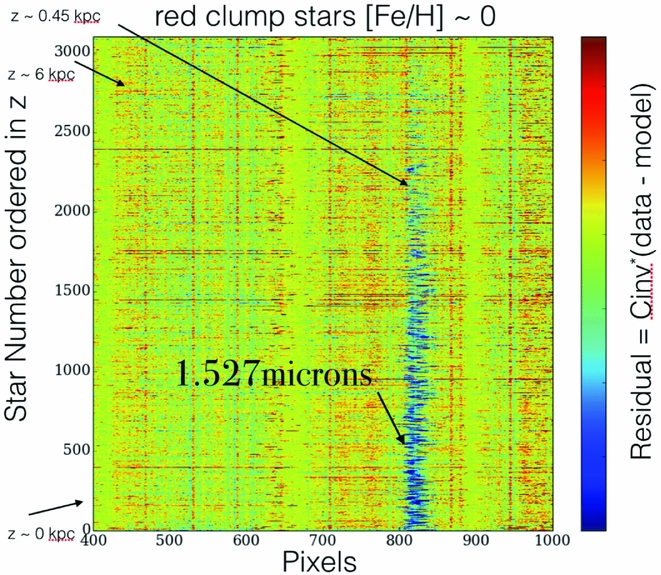
Figure 21. The red clump stars sorted in ascending order of absolute height from the plane |z|, from bottom to top, and coloured by the residual of data model. This figure shows a feature not captured in The Cannon’s model which has high residuals only very near the plane, and is dispersed in radial velocity. This feature corresponds to the strongest diffuse interstellar band identified in the APOGEE spectra (see Zasowski et al. Reference Zasowski, Chojnowski, Whelan, Miroshnichenko, García-Hernández and Majewski2015).
5.3. Where models diverge from data
Comparisons of The Cannon’s model, the data and the theoretical stellar models can inform where stellar models diverge from the data and can be used to correct the stellar models and evaluate the impact of simplified assumptions for example those in 1D, LTE model atmospheres. One example of where the theoretical models diverge from the spectra in the H-band is shown in Figure 22. Both The Cannon’s generative model and the theoretical stellar models (from aspcap) are shown with narrow regions of the APOGEE spectra in this figure. The spectral region in the top right panel of this figure around the log g sensitive Brackett feature demonstrates the poorer fit of the theoretical stellar model (from aspcap’s model grid).
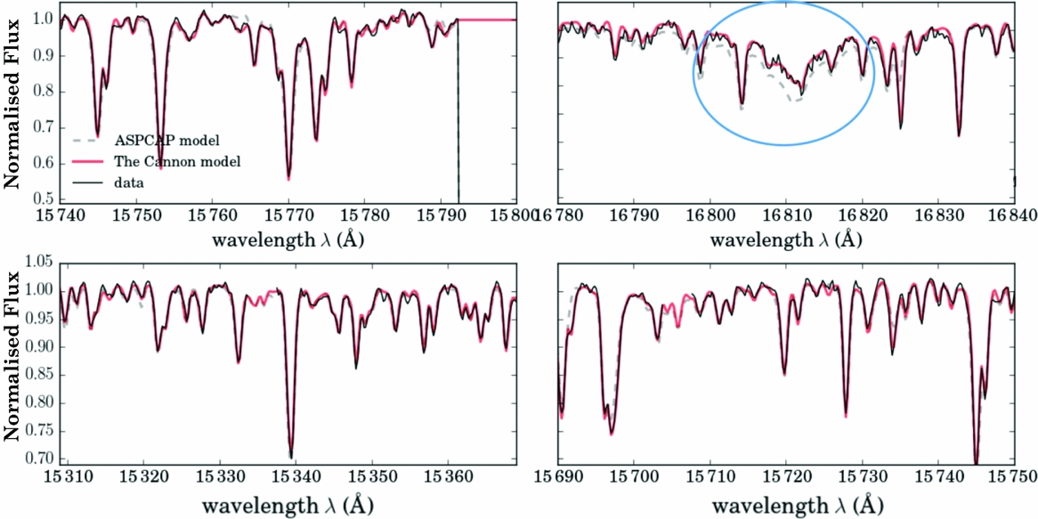
Figure 22. Four narrow regions of the APOGEE spectral regions showing the data (in black), the aspcap model (the dashed line), and The Cannon’s model (in red). The Brackett feature is one region that is poorly fit by the theoretical stellar models as demonstrated in the top right panel. From Ness et al. (Reference Ness, Hogg, Rix, Martig, Pinsonneault and Ho2016b).
The data-driven approach can in fact be used to discover new results that are not covered in the training set. This has been demonstrated in Casey et al. (in preparation), who use deviations from their spectral model from The Cannon around the Lithium line to identify stars that show large deviations in their Lithium abundance, thus discovering the largest set of Lithium enhanced stars known to date.
5.4. Sloan V: Milky Way Mapper
Motivated by success of APOGEE and the performance and new avenues opened up by data-driven techniques, we present what is now a flagship program of Sloan V (P.I. Juna Kollmeier, Kollmeier Reference Kollmeier2017), called Milky Way Mapper (MWM). This program includes the first-ever all-sky, multi-epoch survey of both near-IR and optical spectroscopy of ≈ 5 × 10⁶ stars, that is focused on and contiguous across the disk of the Milky Way. MWM will use the existing APOGEE H-band spectrograph (R = 22,500) augmented with a robotic fiber positioner for rapid reconfiguration. This infrastructure uniquely enables observations of large numbers of stars in the dust-obscured Milky Way disk, where the majority of the stellar mass resides. The selection function for this disk sample is extremely simple and will be a contiguous, complete, magnitude-limited coverage of the disk: fully sampled at H < 11.0, therefore obtaining > 5 million stars spanning a spatial area of > 3000 deg2. The footprint of the expected disc coverage of this survey in azimuthal projection compared to the groundbreaking APOGEE survey is shown in Figure 23. The SNR > 40 (15 min. exposures) requirement of the survey will achieve a precision 0.05 – 0.15 dex for > 20 elements. The disk coverage will be complemented by an all sky coverage of bright stars above the plane to obtain targets being observed for new generation satellite missions including TESS, eROSITA and Gaia that will tie into key questions of stellar physics. The ultimate aim of this next generation spectroscopic survey is to examine the processes that have shaped the Galaxy over an unprecedented range in scale. Specifically, we will address the following with regard to galactic archeology (and many more aspects with respect to stellar physics):
-
(1) What is the chemical and dynamical structure of the disk? We can answer this from what will be the highest dimensional stellar map ever realized (20 elements, ages, 3D velocities, distances)
-
(2) What are the distinct formation and evolutionary histories of our Galaxy? We will be able to determine birth sites and and infer which evolutionary processes drove stars from their birthplaces, using the information we derive.
-
(3) Where does the Milky Way fit into the cosmological context? This extragalactic view of our Galaxy can only be realized by this volume and spatial extent, not the coarse sampling approach of previous generations of surveys nor restriction to completion limited, but only nearby stellar samples.
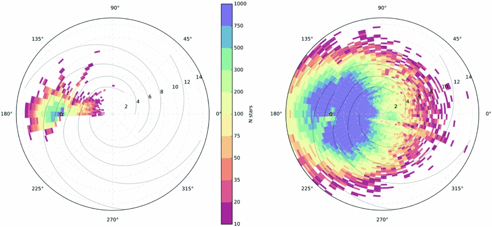
Figure 23. At left, the azimuthal projection of the APOGEE DR12 data release of 250 000 stars and at right the azimuthal projection of the next generation survey of the disk stars targeted by the Milky Way Mapper program within Sloan V's MWM program, showing the >5 million stars in the disk to be observed with contiguous, magnitude-limited coverage. Figure made by Jonathan Bird (Vanderbilt).
6 SUMMARY
In summary, the data-driven methodology of The Cannon is an extremely simple, yet effective approach which relates stellar flux to stellar labels resulting in a method of placing all surveys on the same label scale and delivering labels at 2–3 times improved precision over current approaches. This has opened up new avenues in galactic archeology, delivering masses from stellar spectra across the Milky Way, quantifying the viability of chemical tagging in the resulting regime of high precision and has already placed a multitude of stellar surveys directly on the same scale. There are now approximately one million stars on a single stellar parameter (including some abundances) scale, for the APOGEE, RAVE, and LAMOST stellar surveys. The data-driven approach can further be used in the era of large spectroscopic datasets now upon us to ensure future surveys like GALAH, 4-MOST, WEAVE, and AS4 are directly placed on the same label scale, by observing stars in common between the surveys.
Notably, the label transfer of high-resolution (APOGEE) to low-resolution (LAMOST) surveys has demonstrated the strength in a mathematical approach to derive information from stellar spectra. In particular, this method allows information for individual labels to be extracted from blended features, which are characteristic of low-resolution data. Thus, the information content that can be derived from low-resolution data is actually very high and includes individual abundances at high precision [i.e. C,N; Ho et al. (Reference Ho, Rix, Ness, Hogg, Liu and Ting2016b) and 14 abundances derived in Ting et al. (Reference Ting, Rix, Conroy, Ho and Lin2017)]. It is also likely the data-driven approach can be turned to other datasets, including photometric data and asteroseismic data, in order to further extract the information from these valuable observations and characterise what the information content of this data is. One of the primary applications of The Cannon which has not yet been exploited is to understand where the models diverge from the data, and, to use the data-driven approach to correct theoretical stellar models.
Ultimately, The Cannon is a tool to facilitate understanding of stellar physics and galactic archeology: what is now required for the latter is to develop methodologies and approaches to exploit the independent age, [Fe/H], [α/Fe], and precision [X/Fe] labels derived for surveys and which The Cannon can deliver for stars in future generations of surveys of the Milky Way. Within the next few years (as the data becomes available), more powerful datasets than ever before will be built, with full sky coverage of stellar tracers across the Galaxy, for many millions of stars with precision abundances on the same scale, as delivered with The Cannon given stars in common between different surveys. Coupled with Gaia distances and proper motions, and derived orbit families, the stellar age and individual abundance information provide very strong constraints on the evolution of and birthplace of stars in the Milky Way and represents the ultimate conglomerate of Galactic information (Freeman and Bland-Hawthorn Reference Freeman and Bland-Hawthorn2002).
Freeman and Bland-Hawthorn (Reference Freeman and Bland-Hawthorn2002) asserted that Weinberg’s 1977 statement, that ‘the theory of the formation of galaxies is one of the great outstanding problems of astrophysics, a problem that today seems far from solution’ rang true more than 20 yrs later. However, with the technical progress of the last few years in optimally deriving information from data and the new transformative observational datasets coming online in the coming years, which have been inspired by the lessons of their predecessor surveys, this solution is now very much in reach.
ACKNOWLEDGEMENTS
Thank you to my collaborators whose Figures are reproduced in this proceedings: David W. Hogg, Andrew Casey, Anna Ho, and Jonathan Bird. Thank you to the anonymous referee for their review and input which improved the manuscript. I acknowledge funding from the European Research Council under the European Union’s Seventh Framework Programme (FP 7) ERC Advanced Grant Agreement n. [321035].


