


1. INTRODUCTION
Surface mass balance (SMB), the net mass flux arriving at the ice-sheet surface per unit area, is an important component of ice-sheet mass balance because respective observations or modelling output are used to (i) calculate mass change using the input–output method (Rignot and others, Reference Rignot2008; Medley and others, Reference Medley2014), (ii) to force firn compaction models (Ligtenberg and others, Reference Ligtenberg, Horwath, van den Broeke and Legrésy2012) that can be used to correct altimetry measurements of elevation change (McMillan and others, Reference McMillan2016) and (iii) to identify and partition dynamic ice mass loss when mass change time series are compared against the snowfall deficit into the basin (Hogg and others, Reference Hogg2017). In Antarctic drainage catchments the SMB is usually governed by snow deposition, i.e. snowfall and its re-distribution through drift, as snow melt is only a significant process on ice shelves and the Antarctic Peninsula (Kuipers Munneke and others, Reference Kuipers Munneke, Picard, van den Broeke, Lenaerts and van Meijgaard2012). On Pine Island Glacier (PIG) draining into the Amundsen Sea in West Antarctica there is large heterogeneity in the spatial pattern of SMB, with significantly higher SMB towards the coast in comparison with inland, and an East-West gradient across the basin influenced by topographic features (Lenaerts and others, Reference Lenaerts2018). Over the last 25 years, regional climate models show a cyclical pattern of high (~246 Gt a−1) and low (~154 Gt a−1) SMB years in the Amundsen Sea Embayment, which alternates every 2.5 years on average (Lenaerts and others, Reference Lenaerts2018).
Regional atmospheric climate models such as RACMO (Regional Atmospheric Climate Model; van Wessem and others, Reference van Wessem2018) and MAR (Modèle Atmosphérique Régional; Gallée and others, Reference Gallée2013), or reanalysis products such as JRA55 (the Japanese 55 year Reanalysis; Kobayashi and others, Reference Kobayashi2015) and ERA (European Centre for Medium-Range Weather Forecasts Re-Analysis; Dee and others, Reference Dee2011), presently provide the most commonly used method of estimating the continent wide pattern of SMB in Antarctica. However, while some of these products are able to provide reliable estimates of the magnitude of surface mass input at the basin scale, none are able to resolve the fine spatial pattern of SMB, with the highest resolution continent-wide dataset produced at 27 km resolution (van Wessem and others, Reference van Wessem2018), and a regional product generated at 5.5 km (Lenaerts and others, Reference Lenaerts2018). The spatial resolution of SMB data is important, because it has been demonstrated that lower resolution model output systematically underestimates the rate of snowfall, particularly in relatively mountainous regions (van Wessem and others, Reference van Wessem2016), which may lead to an estimate of the total mass balance that is biased towards more negative values for a glacier catchment. Moreover, SMB models are notoriously poorly constrained by independent observations (Lenaerts and others, Reference Lenaerts2018), due to the logistical effort necessary for collecting measurements for one season in Antarctica, let alone over longer time periods, so that the total amount of snow deposition across the full range of spatial scales remains uncertain.
New in-situ observations of snow deposition at point locations can be acquired using an automatic weather station (e.g. Colwell and others, Reference Colwell, Keller, Lazzara, Setzer and Fogt2015), ice cores (e.g. Sigg and Neftel, Reference Sigg and Neftel1988), a neutron probe (e.g. Morris and Cooper, Reference Morris and Cooper2003), snow pits (e.g. Parry and others, Reference Parry2007), cosmic rays (e.g. Howat and others, Reference Howat, de la Peña, Desilets and Womack2018), GPS reflectometry (e.g. Siegfried and others, Reference Siegfried, Medley, Larson, Fricker and Tulaczyk2017) and stake farms. Measuring SMB using the horizontal variability of stratigraphy in the firn pack, whether through ground-based or airborne radar (Medley and others, Reference Medley2014), provides an opportunity to study the heterogeneous pattern of SMB over different spatial scales, from a few metres to hundreds of kilometres. On PIG, radar-derived SMB estimates have been reported before over various periods (Vaughan and others, Reference Vaughan, Bamber, Giovinetto, Russell and Cooper1999; Karlsson and others, Reference Karlsson2014; Medley and others, Reference Medley2014), but these cover only small parts of the fast flowing areas of PIG due to less continuous radar echoes (Karlsson and others, Reference Karlsson, Rippin, Vaughan and Corr2009) and spatial sampling.
Inferring the SMB from the stratigraphy in the firn and ice body is based on dividing the mass in the vertical column between the upper and lower boundaries of a layer, which is related to the layer's thickness, by the age difference at these boundaries. However, the mass or thickness of a layer contained within the glacier does not only depend on the amount of snow deposited, but also on firn and ice dynamics (Ng and King, Reference Ng and King2011). Glaciers flowing from an ice divide in the centre of an ice sheet towards their ablation areas or – in the case of Antarctica – their interface with the surrounding ocean, exhibit different strain regimes depending on local flow conditions. In areas of horizontally compressive flow, ice thickness and likewise annual layers experience a net thickening; in areas of horizontally extending flow, they undergo a net thinning (Cuffey and Paterson, Reference Cuffey and Paterson2010). This affects the mass of snow, firn or ice measured along the length of a core, between the glacier surface and a radar-derived internal layer, or between several layers, and consequently the SMB estimate that comes from such dated layer thickness information. In an area of net thickening, the SMB may be overestimated by simply dividing mass, or layer depth, by layer age, whereas conversely the SMB in thinning areas may be underestimated. Based on assumptions about flow velocities, the strain history that a firn parcel experiences on its path can be estimated and corrected (e.g. Dansgaard and Johnsen, Reference Dansgaard and Johnsen1969 and applications thereof, e.g. Fahnestock and others, Reference Fahnestock, Abdalati, Luo and Gogineni2001; Lilien and others, Reference Lilien2018) so that the parcel's mass at deposition, i.e. the respective SMB, can be derived. In complex situations where respective assumptions would not hold anymore, or over long time periods, another way of interpreting the internal stratigraphy is to compare it with forward-modelled layering based on numerical models of ice dynamics (e.g. Karlsson and others, Reference Karlsson2014). Usually, accounting for the strain history is thought to be necessary only beyond a certain depth depending on flow conditions (Waddington and others, Reference Waddington, Neumann, Koutnik and Marshall2007) and negligible for near-surface layers at depths of only tens of metres so that strain corrections are not usually applied (e.g. Eisen and others, Reference Eisen2008; Hawley and others, Reference Hawley2014; Medley and others, Reference Medley2014). However, highly dynamic areas specifically exempted by Eisen and others (Reference Eisen2008) as regions where strain becomes relevant, such as the relatively fast flowing tributaries and main trunk of PIG (Fig. 1), remain largely unprobed in this respect because the internal stratigraphy is often discontinuous or missing entirely in radar records in these areas (Karlsson and others, Reference Karlsson, Rippin, Vaughan and Corr2009) and ground truth in the form of ice core observations are usually sampled only near ice divides far off the fast flowing ice streams.
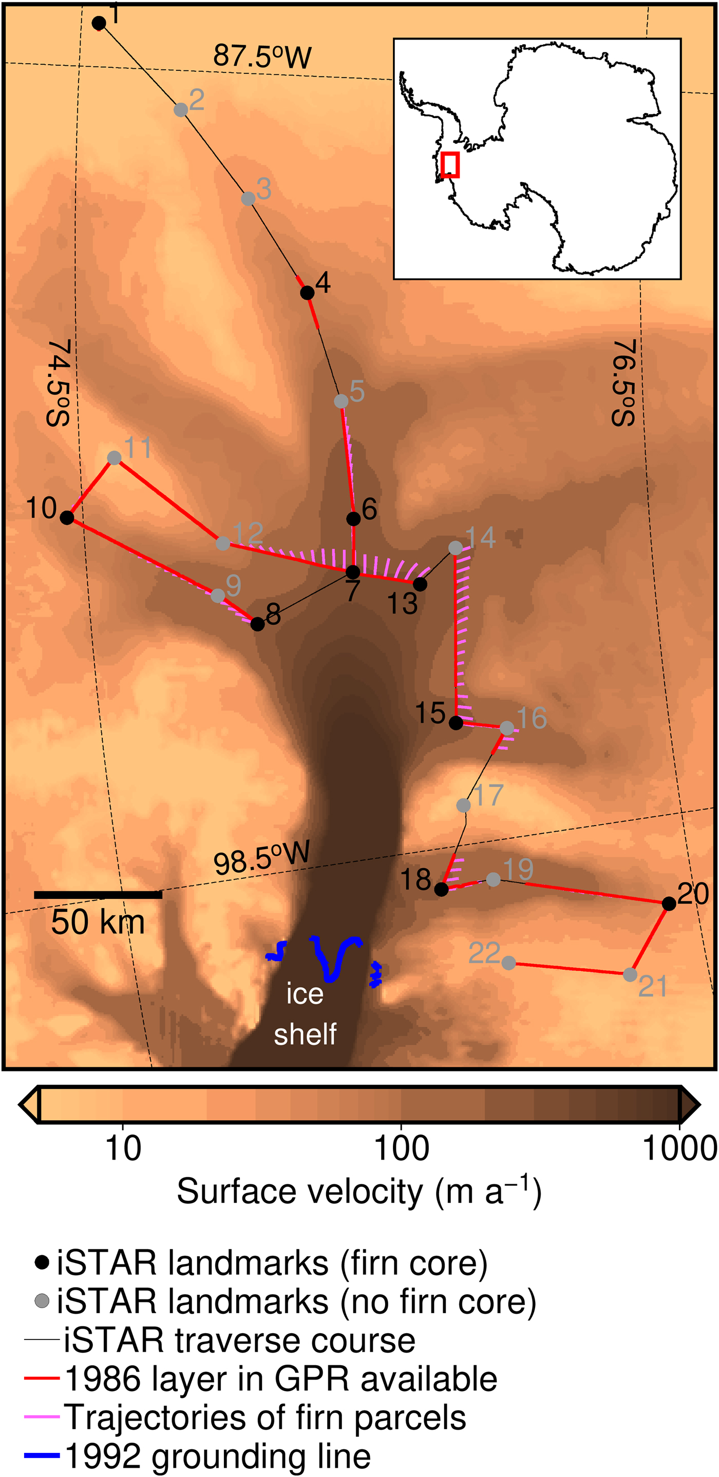
Fig. 1. Overview map of the iSTAR traverse on PIG as given by the 22 landmark sites. The location of PIG in Antarctica is indicated by the red square in the top right inset. SMB estimates are retrieved where the 1986 layer is available along the traverse. The trajectories of firn parcels indicate the path from the source location to the record location along the traverse (1986–2014). The magnitudes of the surface velocity field (Arthern and others, Reference Arthern, Hindmarsh and Williams2015) are shown as the background image on a saturated logarithmic scale, and the grounding-line position in 1992 is also illustrated (Park and others, Reference Park2013).
In this study, we combine ground-penetrating radar (GPR) data and shallow (<50 m) firn cores to retrieve a new dataset of SMB on PIG, sampling fast and slow flowing areas around the main trunk alike. The data were collected on the Natural Environment Research Council's (NERC) ice sheet stability programme (iSTAR) land ice traverse in the austral summers of 2013/14 and 2014/15 (Fig. 1). A reflector in the GPR record that is consistent along much of the traverse was identified. The travel times of the recorded radar echo were converted into water equivalent (w.e.) depth using density profiles of the firn cores. Analysis of photosynthetic chemicals in the firn cores was used to reliably date the onset of snow deposition of the layer confined by the glacier surface and the picked reflector. Combined, this dataset provides high spatial resolution observations of the rate of SMB across much of the PIG catchment over the time 1986–2014. We then correct the derived SMB for the strain history of the mapped layer in the radar data. Common one-dimensional approaches, such as the one by Dansgaard and Johnsen (Reference Dansgaard and Johnsen1969), assume certain vertical profiles of horizontal flow velocities. These approaches are valid only for horizontally uniform ice thickness and SMB – conditions more likely met where ice flows slowly and a parcel does not travel through present gradients fast enough for them to change the respective surface burial rate or strain regime. We apply a strain correction that overcomes these restrictions and is thus able to identify areas where the dynamics of PIG affect SMB estimates based on firn stratigraphy significantly through the strain history, even in the relatively short period 1986–2014. Finally, we assess whether accounting for the strain history of a previously published basin-wide cumulative SMB (Medley and others, Reference Medley2014), changes the estimate of the basins total mass balance.
2. METHODS
2.1 Ground-penetrating radar
The record of firn stratigraphy via GPR was acquired in the field season of the 2013/14 Antarctic summer during the first of two iSTAR on-ice campaigns. A commercially available pulseEKKO PRO system operating at 100 MHz was deployed in common-offset mode, allowing for a vertical resolution of ~1 m (or 10 ns). The transmitting and receiving antennas were placed on sleds and towed behind the campaign's tractor train along the 900 km traverse, moving at an average speed of ~10 km h−1 with one sample collected every ~1.4 m. The positioning of single radar traces along the traverse is done via GPS measurements at the radar antennas, and – where these failed – at the main compartment of the train. In each leg of the traverse, the processing of the raw radar data encompassed a static correction, bandpass filtering, background removal and a gain correction, all carried out using commercial REFLEXW software. In the upper part of a polar firn and ice bodies, such internal reflectors have been found to originate mainly from the density-driven contrast in the dielectric permittivity of the firn (Eisen and others, Reference Eisen, Wilhelms, Nixdorf and Miller2003) and can be considered to represent isochrones within the firn and ice body due to the common timing of formation (Spikes and others, Reference Spikes, Hamilton, Arcone and Kaspari2004). With a focus on multi-decadal, satellite-era coverage of our SMB estimate and having in mind our later goal to compare our results with those by Medley and others (Reference Medley2014), we aimed to retrieve the depth of an isochronous layer from around the mid-1980s. Therefore, a prominent reflector formed around this age was picked by eye in the radargrams (Fig. 2) wherever possible. The travel times of the radar echoes were converted into depth according to an empirical relationship (Kovacs and others, Reference Kovacs, Gow and Morey1995) between the dielectric permittivity of firn and the depth-dependent firn density from the firn cores (see Section 2.2 and Fig. 3). Then, the layer depth was converted into w.e. depth, again using the density along the firn cores. In both instances, we used the mean firn density profile (Fig. 3) obtained by averaging the density at the ten core locations at a given depth, after linearly interpolating to a common depth scale. Due to corrupted or missing data, there are several gaps in the record (Fig. 1). The chronologies in the firn cores together with the travel-time-to-depth conversion based on density measurements of the firn cores helped to detect the respective layer where such gaps prevented continuous tracking and to identify the reflector from the mid-1980s in the first place. Larger gaps mainly exist where an intact record of firn stratigraphy could not be connected to a firn core, such as around sites 2 and 3 (Fig. 1).
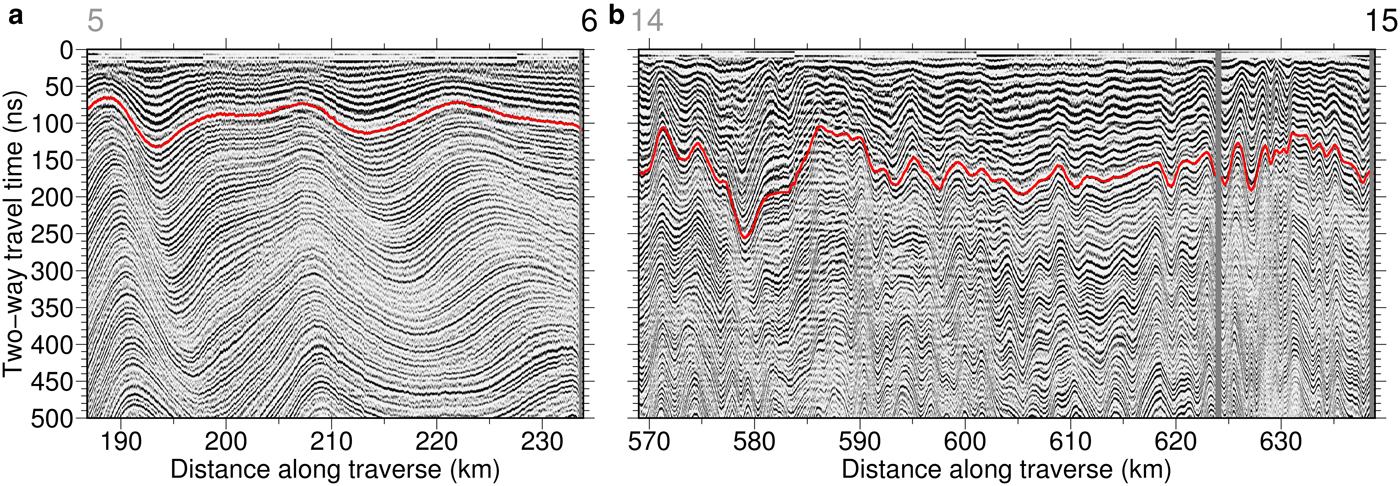
Fig. 2. Radargrams along the selected sections of the traverse. (a) Along flow, featuring relatively smooth variations in reflector depth; the ice flows from left to right. (b) Across a shear margin, featuring a disturbed stratigraphy, i.e. sharp transitions in reflector depth and extensive layer convergence and divergence. The greyscale colour code represents amplitudes of the recorded radar echoes. Landmark sites of the iSTAR traverse are indicated by their number above the radargrams, see also Figure 1 for their locations on PIG. Black labels indicate those which feature a firn core, grey those which do not. The red line represents the picked reflector from ~1986 (see the main text and Table 1). According to the mean density distribution (Fig. 3) and the applied empirical relationship between firn density and propagation speed of electromagnetic radiation in firn (Kovacs and others, Reference Kovacs, Gow and Morey1995), a travel time of 10 ns approximately equals 1 m depth.

Fig. 3. Firn density as a function of depth in the ten firn cores (see their locations in Fig. 1) and their respective mean and std dev.
Table 1. Depth and dating (column ‘year') of the picked layer at the firn core locations on the iSTAR traverse, and the respective dating average, from which the average age in years can be obtained by subtracting from 2014. Site 10 has been excluded from the average (see the main text). The average uncertainty comprises both the average uncertainty and the variability of the ages at the different sites (see the main text)

2.2 Firn cores
During the second iSTAR campaign in the 2014/15 Antarctic summer, ~50 m deep firn cores were drilled at ten of the traverse's landmark sites (Fig. 1). Hydrogen peroxide contained in the firn was measured in a continuous flow analysis, and annual summer peaks in this parameter were identified and used to determine each site's age-depth relation (Sigg and Neftel, Reference Sigg and Neftel1988). The year of accumulation of the deepest parts of the firn cores varies from site to site between 1921 and 1983, depending on the local SMB conditions and thus average burial rates. The chronologies were offset by 1 year in order to compensate for the different acquisition times of the GPR and firn-core data, and the dating uncertainty associated with this shift was assumed to be 1 year. The density–depth profiles (Fig. 3) of the ten firn cores were obtained gravimetrically, i.e. by measuring the mass of firn core sections of varying length, with a median length of ~32 cm.
2.3 Strain correction
A strain correction aims to retrieve the initial mass or thickness, respectively, of a parcel in a glacier at the time of deposition based on its measured thickness at a later time and on the velocity field that it travelled through along its path  ${\mathop{ r}^{\hskip -5pt \rightharpoonup}} (t)$, thus experiencing a mass gain or depletion due to the related strain. Here, we derive the strain correction for such a firn parcel. Its vertical extent, converted to ice equivalent, is h. The firn parcel's mass is conserved by balancing the horizontal and vertical dimensions of the parcel if it experiences strain. According to Eqn (A20) in Jenkins and others (Reference Jenkins, Corr, Nicholls, Stewart and Doake2006), this can be expressed as
 $$\displaystyle{{{\rm d}h} \over {{\rm d}t}} = -\underbrace{{\left( {\displaystyle{{\partial u} \over {\partial x}} + \displaystyle{{\partial v} \over {\partial y}}} \right)}}_{{{\rm div}\; {\vec{u}}_{\rm h}}}\; h.$$
Here, x and y are the horizontal Cartesian coordinates, and u and v are the respective components of the ice velocity field at the surface;  ${\rm div}\; \vec{u}_{\rm h}$ is the divergence of the horizontal surface velocity field. We simplified the original expression by Jenkins and others (Reference Jenkins, Corr, Nicholls, Stewart and Doake2006) because there is no mass flux through the upper (‘u’) and lower (‘l’) boundaries of the parcel ( $\dot{m}_{\rm u} = \dot{m}_{\rm l} = 0$). Additionally, we assume that horizontal flow velocities do not change with depth close to the glacier's surface, i.e. the velocity anomalies with respect to depth, v ′, u ′ are zero; see below for the validity of this assumption. Finally, because we consider ice equivalent vertical extent, we assume a constant density $\bar{\rho} $, allowing us to eliminate it from the equations. By integrating Eqn (1) along the parcel's path ${\mathop{ r}^{\hskip -5pt \rightharpoonup}} (t)$, its thickness at time t is related to its thickness at deposition at time t d by
 $$h\left( {t_{\rm d}} \right) = h(t)\cdot \underbrace{{{\rm e}^{-\int_{t_{\rm d}}^t {{\rm div}\; {\vec{u}}_{\rm h}\left(\, {\mathop{r}^{\hskip -4pt \rightharpoonup} \left( {{t}^{\prime}} \right),{t}^{\prime}} \right)\; {\rm d}{t}^{\prime}} }}}_{{\alpha (t)}}$$
Here, α represents the thickness at time t relative to the thickness at time t d. The layer between the surface and the picked isochronous reflector from the GPR analysis comprises firn accumulated at various times between the time of GPR acquisition, t a, and the time from which the reflector originates, t 0, so we average α along the parcel's path:
 $$\bar{\alpha} = \displaystyle{{\mathop \int \nolimits_{t_0}^{t_{\rm a}} \alpha \lpar t \rpar {\rm d}t} \over {t_{\rm a}-t_0}}.$$
 The total mass of snow, firn or ice in terms of ice-equivalent thickness in the acquired radar image of the englacial stratigraphy, which has been deposited along the path towards the location along the GPR profile over the period between t 0 and t a, can then be obtained by multiplying the ice-equivalent depth of the picked reflector with the strain correction factor  $\bar{\alpha} $. As the conversion from ice- to w.e. thickness involves only a multiplication by a constant factor, the same operation works for w.e. thickness as retrieved in our GPR processing (Section 2.1). In the numerical implementation of the integrals Eqns (2) and (3), the time increment was 0.1 years.
Here, we use the surface velocity field by Arthern and others (Reference Arthern, Hindmarsh and Williams2015) obtained from an ice-dynamical model, for which, among others, velocity observations derived from satellite radar interferometry (Rignot and others, Reference Rignot, Mouginot and Scheuchl2011) have been assimilated, for both computing the divergence of the horizontal surface velocity field and determining the trajectories of the firn parcels  ${\mathop{ r}^{\hskip -5pt \rightharpoonup}} (t)$ in Eqn (2) as surface flowlines. The velocity field (Fig. 1) is available at a resolution of 2 km. We interpolate both the horizontal velocity components and the divergence bilinearly to the trajectories ${\mathop{r}^{\hskip -5pt \rightharpoonup}} (t)$ at the 0.1 years intervals. We prefer this synthetic data set over the original observations by Rignot and others (Reference Rignot, Mouginot and Scheuchl2011) because the respective divergence (Fig. 4) has no data gaps, and is free of artefacts from the mosaicking of satellite images which proved to have strong effects on our results in some places when utilising these original observations. Relative changes of velocity with depth in the Arthern and others (Reference Arthern, Hindmarsh and Williams2015) model in the uppermost 50 m are <0.1%, confirming that the assumption of vertically uniform flow velocities holds in the model.
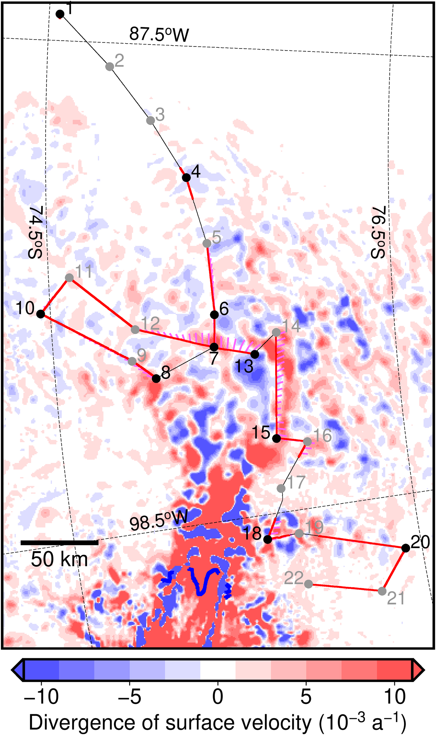
Fig. 4. Divergence of the surface velocity field (Arthern and others, Reference Arthern, Hindmarsh and Williams2015, see also Fig. 1). Apart from the displayed divergence field, the same legend as in Figure 1 applies: the iSTAR traverse (data collected (red line), and no data (black line)), iSTAR landmark sites with firn core available (black circle) and without firn core (grey circle), firn parcel trajectories (purple lines) and the 1992 grounding line position (blue line) are also illustrated. According to Eqn (1), a firn parcel will experience thinning when travelling through red areas (positive divergence) and thickening in blue areas (negative divergence).
Together with the respective upstream particle paths, Eqns (2) and (3) provides us with strain correction factors  $\bar{\alpha} $ for all locations where the dated reflector is available. We do not consider vertical firn compaction here as this is already implied when converting the depth of the reflector into w.e. depth via the mean regional firn density profile. As a by-product of this analysis, we retrieve the upstream advection correction for deposited snow from the GPR profiles to its source location, i.e. its trajectory according to the considered velocity field (Fig. 1).
We also assess the effect of this strain correction on an earlier SMB estimate (Medley and others, Reference Medley2014). This SMB estimate was obtained from a similar combination of airborne radar-derived isochrone depths and dating using established local firn chronologies, extrapolated onto a uniform grid (3 km spacing) using kriging. We apply the above formalism of upstream advection and integration of strain history to each grid cell's value, at the respective centre of each grid cell, by considering the time window of Medley and others (Reference Medley2014) for averaging SMB (1985–2009). Using this method we are able to quantify how the strain correction affects the estimate of total SMB integrated over the catchment of PIG.
By tracing the flowlines implied by the velocity field the strain rate corrections can be made, even where advection carries the firn parcel through a complicated strain field caused by flow of the ice over undulating bed topography. Using this approach, it is possible to correct for the net effect of multiple instances of strain-driven thickening and thinning along a flowline. Through this, our approach overcomes limitations of common local, i.e. one-dimensional, approaches such as the one by Dansgaard and Johnsen (Reference Dansgaard and Johnsen1969), which becomes invalid if a parcel travels through spatial gradients of SMB or ice thickness long enough for its depth being affected by the varying burial rate due to spatial variations of SMB or for different strain regimes contributing to similar extents to the change in its vertical thickness (Waddington and others, Reference Waddington, Neumann, Koutnik and Marshall2007). Our approach is, however, limited by the accuracy of the horizontal divergence computed on the basis of a given velocity field. The accuracy is, for example, diminished by the model-implicit additional assumption that the velocity field does not change over time, despite observed acceleration of PIG's tributaries over recent decades (Mouginot and others, Reference Mouginot, Rignot and Scheuchl2014). Also, if our approach was extended to layers at greater depth, variations of the horizontal velocity field with depth would need to be included, as is done in local, one-dimensional models or more sophisticated thermomechanical models of particle paths and strain history (e.g. Waddington and others, Reference Waddington, Neumann, Koutnik and Marshall2007).
3. RESULTS AND DISCUSSION
3.1 Layer depth and age
The travel-time conversion of the picked reflector according to the average firn-density profile resulted in a depth range of 5.5–31 m w.e. The chronologies of the firn cores were evaluated at these respective depths (Table 1), and the respective reflector was found to stem from 1986, approximately coinciding with the main reflector tracked by Medley and others (Reference Medley2014) who examined SMB based on a reflector from 1985. It is important to note that the reflector-picking strategy in disconnected sections of the traverse relied on the established firn core chronologies (see above), so that the age of the reflector would be consistent over the whole traverse. In this sense, the ages determined in the different firn cores are independent only where two or more cores are connected, i.e. the area defined by sites 05–13. The uncertainty in the depth of the picked reflector and the inherent dating uncertainty of 1 year (see above, offset between firn core and GPR acquisition) go into the respective uncertainties at the individual firn-core sites. The uncertainty of the average reflector age,  $\overline {\Delta t} = \sqrt {{\overline {\delta t}} ^2 + \delta {\bar{t}}^2} = \; 1.2$ years (Table 1), comprises both the average dating uncertainty at the individual firn-core sites, $\overline {\delta t} $, and the std dev. of the dating at the different firn-core sites, $\delta \bar{t}$.
The chronology at site 10 was classed as anomalous because the layer age did not match the ages at connected locations (6, 7, 8 and 13, see Table 1). Repeated analysis of the reflectors in the GPR data revealed that it is not the layer tracing strategy that fails here. As the hydrogen peroxide analysis was also not feasible beyond 40 years or 8.7 m w.e. depth at site 10, we assume that the chronology at this site might be perturbed by loss of annual snow or a spatial or temporal bias in the sampled snow and firn. Therefore, the retrieved layer age at site 10 does not go into the inter-firn core average age assigned to the reflector.
3.2 Uncorrected surface mass balance
A first estimate of SMB was obtained by dividing the w.e. depth of the picked reflector by the age of the reflector. This SMB estimate (Fig. 5a) does not yet take into account the strain history of the firn column between the glacier surface and the picked reflector. Over the whole iSTAR traverse, PIG received an average 0.505 m w.e. a−1 of surface mass between 1986 and 2014, with the maximum and minimum SMB of 1.108 and 0.195 m w.e. a−1, respectively. Our observations show an increase in SMB from the northern and eastern area of PIG (0.2–0.5 m w.e. a−1, sites 1–13) towards the southwestern region (0.5–1.0 m w.e. a−1, sites 14–22) close to the boundary with Thwaites Glacier. The spatial distribution of SMB is in general agreement with earlier findings from regional climate modelling and airborne radar surveys (Arthern and others, Reference Arthern, Winebrenner and Vaughan2006; van de Berg and others, Reference van de Berg, van den Broeke, Reijmer and van Meijgaard2006; Medley and others, Reference Medley2014; Lenaerts and others, Reference Lenaerts2018). The above mean SMB in our dataset is higher than the mean value estimated by these earlier modelled or observed datasets, because the iSTAR traverse preferentially sampled this region of particularly high accumulation towards Thwaites Glacier. The spatial variability of the retrieved SMB is highest where the traverse passes through shear margins (Fig. 2b). Here, the distorted stratigraphy and derived SMB is more likely to be produced by horizontal stress gradients than by actual spatial variations in snow accumulation (Leysinger Vieli and others, Reference Leysinger Vieli, Hindmarsh and Siegert2007), indicating that a correction for experienced strain is necessary here.
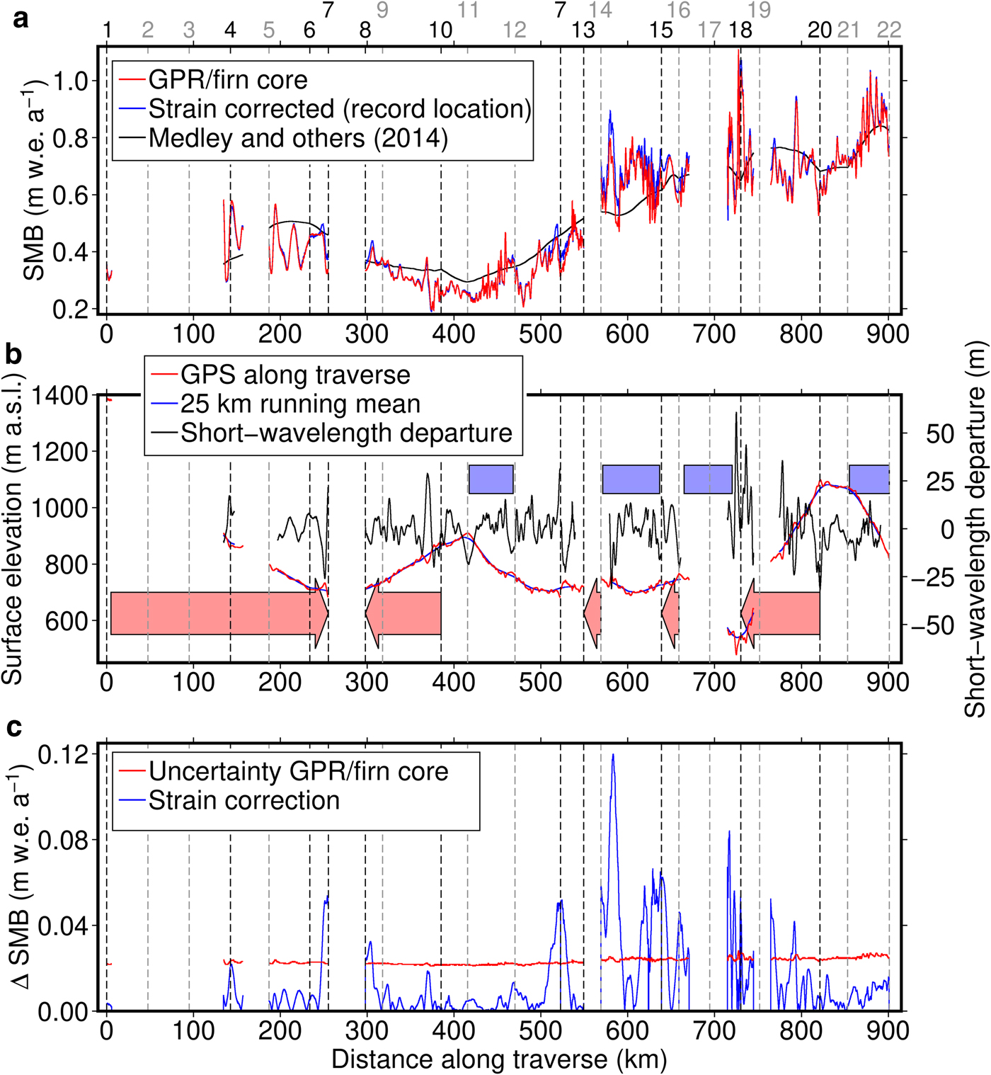
Fig. 5. (a) SMB along the iSTAR traverse; uncorrected for strain (i.e. simply w.e. depth divided by age, red), strain-corrected (through upstream advection) but displayed at the record locations (see the main text; blue) and the gridded regional product by Medley and others (Reference Medley2014) (black). Note that the latter is not corrected for its strain history here. (b) Surface elevation (red, left axis), its 25 km running mean (thin blue, left axis), and the short-wavelength departure of surface elevation from the running mean (black, right axis) along the traverse. Where the traverse travelled in the along flow direction, this is indicated by the light red arrows (pointing in the flow direction); blue bars indicate shear margins. (c) Uncertainty of the uncorrected SMB (red; caused by the ambiguity of layer detection, and by the uncertainty in the wave speed, i.e. firn density and layer age, see the main text), and the effect of the strain correction (blue). The latter is effectively the absolute difference between the red and the blue line in (a). Vertical dashed lines mark the iSTAR traverse landmark sites (Fig. 1), where firn cores were collected at sites annotated in black and not collected at sites annotated in grey.
Compared with these strong disruptions on short spatial scales, the spatial pattern of SMB varies over longer spatial scales (~10 km) where the traverse travelled in the along flow direction on the main ice stream tributaries (e.g. in the sections flowing from site 4 to 7, from 16 to 15, from 10 to 9, Figs 1, 5). This pattern is also reflected in the ice surface elevation, or its deviation from the respective 25-km running mean of the topography (Fig. 5b). Features in the ice sheet surface topography are most likely to be formed where the glacier overrides prominent peaks in the bedrock topography, and connections between features in the bedrock and surface topographies have been reported in this region of PIG (Bingham and others, Reference Bingham2017). On the Siple Coast, such features in the surface topography have been shown to affect the local SMB through modulation of the snow drift caused by variable surface winds (Arcone and others, Reference Arcone, Spikes and Hamilton2005). Ng and King (Reference Ng and King2011) describe how GPR-observed isochronous layers that are caused by variations in SMB develop as kinematic waves as they submerge and are transported downstream. Such downstream migration of highs and lows in the internal firn stratigraphy are also present in our GPR record from PIG (Fig. 2a). Therefore, we hypothesise that these along-flow, undulating variations in the internal stratigraphy at spatial scales of ~10 km represent real spatial variability in SMB, driven by the glacier geometry and stratigraphically modulated by the ice flow. This spatial variability indicates that the annual layer thickness and therefore SMB obtained from the firn cores alone could be affected by upstream effects, which must be carefully corrected in order to retrieve a more robust record of the real temporal evolution of SMB from the firn-core records in future studies. Otherwise, trends with depth in the firn core records may be falsely attributed to temporal variability, when in fact spatial gradients are the cause of these trends. Similar spatial variability can be expected in traverse sections that are not along flow, but it is often masked by the layer disruptions on shorter spatial scales and, due to the radargrams not following the flow direction, cannot be linked to the kinematic behaviour discussed by Ng and King (Reference Ng and King2011) and seen in Figure 2a.
Uncertainties of the radar-derived SMB take into account the dating uncertainty (1.2 years; Table 1), the vertical resolution provided by the radar wavelet which is controlled by the wavelength (10 ns or ~1 m; Navarro and Eisen, Reference Navarro, Eisen, Pellika and Rees2009), and the std dev. of the regional firn density mean per depth (5–50 kg m−3; Fig. 3) used to compute the radar wave speed in firn. The uncertainty amounts to ~0.026 m w.e. a−1 (Fig. 5c), where the two sources of uncertainty (age and depth) make similar contributions of ~0.018 m w.e. a−1. It should be noted that, at least on PIG, (local) variations in the density–depth relationship are generally expected to have a negligible cumulative effect of only ~5 cm on the retrieved radar-derived depth in the uppermost 12 m (Morris and others, Reference Morris2017) and likely also beyond. An unaccounted error source lies in the empirical relationship used to convert density into dielectric permittivity.
3.3 Impact of strain correction
Starting at the place where it has been deposited (referred to as ‘source location’ hereafter), any firn parcel observed along the GPR profiles has travelled to its current location on the iSTAR traverse (referred to as ‘record location’ hereafter) with the glacier's flow. The strain correction that we apply to such a parcel involves an upstream correction, too, which aims to reconstruct this path and respective local strain rates (see Section 2.3). Within the limitations of this approach (i.e. a vertically and temporally constant velocity field), we are consequently able to allocate respective (strain-corrected) SMB estimates to their source locations. However, the additional information of the source locations makes the analysis and illustration of the results impractical: first, the source location is not confined to the one-dimensional traverse path implying a very different sparse data set compared with the original GPR record. This makes the more sophisticated approach of retrieving accumulation rate and source location based on layer depth and record location such as in Eqn (18) by Ng and King (Reference Ng and King2011) unfeasible for long sections of our data. Second, the source location for any parcel is ambiguous because the firn present in a vertical column of finite thickness is not accumulated at a single, unique location but along the path of the oldest (i.e. deepest) parcel in the column over the 28 year period. Therefore, we opt for displaying and analysing the respective results at the record locations, i.e. along the GPR-covered traverse. This enables us to plot and compare uncorrected and corrected SMB estimates along-side each other at their unique record locations. It is, however, important to note that the correction implies the upstream advection of firn parcels; the strain history could not be estimated without the upstream advection in our approach.
The maximum distance between source and record locations of 8 km over the 28 years is reached around iSTAR sites 7 and 13 (Fig. 1), located close to the main central trunk of PIG. Our results show that along 66.6% of the traverse, where data were collected, the strain correction is less than half of the SMB uncertainty, and along 79.8% of the traverse it is less than the full SMB uncertainty (Fig. 5c). The strain correction exceeds the SMB uncertainty around site 7 which is located at the confluence of several tributaries into the central fast flowing trunk of PIG, where ice velocities are highest along the traverse and therefore the distance between source and record locations of firn parcels through areas of strain thinning are longest (Fig. 4). The strain correction is also higher than the observed data uncertainty between site 14 to halfway between sites 19 and 20, where the traverse crosses the shear margin of two tributaries. The maximum strain correction, calculated as ~0.12 m w.e. a−1, ~4.9 times the local observational uncertainty, was measured just after iSTAR site 14 where the traverse entered a faster flowing PIG tributary via an inter-tributary shear margin, and where the ice surface velocity field indicates strong thinning (Fig. 4). These results suggest that while locally significant, the strain correction is negligible over long sections of the traverse as the absolute difference between uncorrected and corrected SMB is below the measurement uncertainty (Fig. 5c).
While the strain correction in the shear margin near site 14 is well above the nominal SMB uncertainty, it remains negligible in the well-sampled shear margin between site 11 and 12 and at the boundary to Thwaites Glacier between sites 21 and 22, also visible in the near-zero flow divergence in these areas (Fig. 4). The traverse passed through one more shear margin around site 17, but the reflector could not be traced in this part in the GPR record. Low divergence as around sites 11, 12, 21 and 22 (Fig. 4) indicates that the strain correction would be small here, too. The distortion of the stratigraphy is most likely caused by horizontal gradients in stress (see Section 3.2). Our strain correction does not restore the supposedly smoother pattern of the initial snow deposition, indicating that it does not capture the deformation leading to these disruptions and thus the full strain regime in the shear margins, possibly due to violations of the underlying assumptions (vertically and temporally uniform model-derived flow field).
It is evident from the divergence field in Figure 4 that there is no simple way to characterise the respective correction as a firn parcel could experience a sequence of thinning and thickening due to ice divergence as it flows along the glacier, or none at all, depending on the location of its travel path. According to our analysis, the uncorrected SMB on PIG is generally lower than the corrected SMB estimate because the traverse goes through more thinning (negative divergence, Fig. 4) than thickening patches (positive divergence). The upstream advection correction depends on the duration of a parcel's exposure to strain (Eqn (2)), which means that the strain correction would be even smaller if a more recently deposited layer within the firn body had been selected, or conversely it would be larger if an older, and consequently deeper stratigraphic layer was selected. Overall, because the strain correction proves to be generally smaller than the observational uncertainty, our results suggest that the correction of observations of SMB covering the most recent 30 years for the effects of strain is mostly, but not universally, negligible in places subject to similar conditions as PIG in terms of average SMB and ice flow. In general and not only restricted to an analysis on PIG, we advise to estimate  $\bar{\alpha} $ in Eqn (3) for a range of possible paths representative for a larger part of the studied region in order to assess at which length of a record one would need to apply strain corrections. These, together with average SMB estimates, can indicate if the strain corrections might exceed the observational uncertainty. It should be kept in mind that the underlying assumptions (vertically and temporally uniform flow velocity, model output based on data assimilation as a good representation of the actual velocity field) may be violated and thus not applicable when applying our approach to other glaciers.
3.4 Comparison with SMB estimate from airborne radar data
We used our in-situ GPR observations (not corrected for the strain history) to assess a SMB estimate covering the period 1985–2009, derived from airborne radar observations which have smaller coverage over the fastest flowing sections of the PIG drainage catchment. We evaluated a map of mean SMB between 1985 and 2009 (Fig. 6a, Medley and others, Reference Medley2014) using bilinear interpolation along the iSTAR traverse (Fig. 5a). This comparison shows that the map has the same broad-scale spatial pattern of SMB across the PIG basin as the in-situ observations (Fig. 6a), implying consistency between the two records and the climatological processes mutually observed by them. However, due to the coarser resolution of the airborne data, and the smoothing performed in the data processing, the map does not retain the small spatial scale SMB variations seen in the unsmoothed in-situ observations. The result of this is up to 0.2 m w.e. a−1 underestimation (site 04, between 14 and 15, towards 22) or overestimation (sites 5 to 7, 10 to 13, 19 to 20) of the broad SMB pattern, regardless of whether or not the strain correction is applied. As the airborne observations (Medley and others, Reference Medley2014) only cross the iSTAR traverse in a few locations (Fig. 6a), the differences between the SMB amplitudes may be in part caused by the kriging scheme used by Medley and others (Reference Medley2014) to extend the SMB estimates from the radar flight lines to the entire basin.
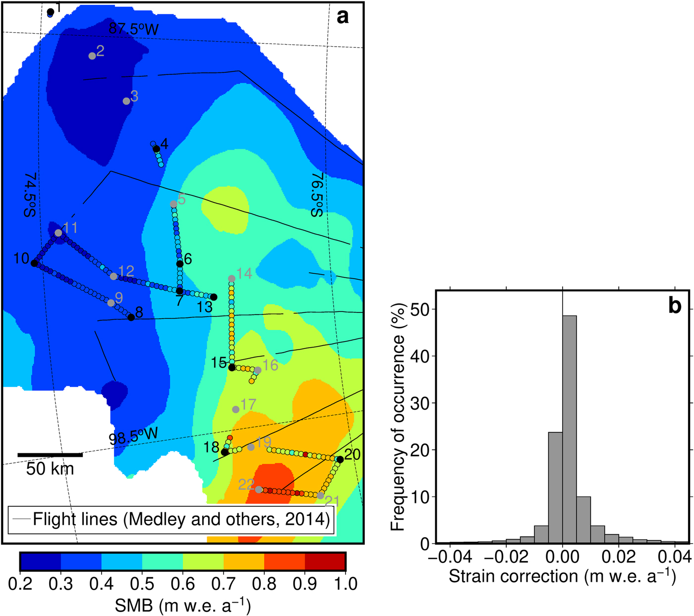
Fig. 6. (a) Map of average SMB in the PIG basin between 1985 and 2009 (Medley and others, Reference Medley2014; not corrected for its strain history). For comparison, the SMB from this study, also not corrected for strain, is plotted on top of the map as colour coded circles every 3.5 km. Black lines indicate the locations from which airborne SMB observations were interpolated across the study area. (b) Distribution of the difference between uncorrected and strain-corrected SMB against the gridded SMB map (Medley and others, Reference Medley2014) in each of the 3 km by 3 km grid cells inside the PIG catchment. Positive difference means that the corrected SMB is higher than the uncorrected one, i.e. the respective firn column has experienced a net thinning over time.
3.5 Off-traverse strain corrections and basin-wide integration
Finally, we assessed the impact of the strain correction on the gridded map of SMB by Medley and others (Reference Medley2014), and the effect this has on the estimate of total surface mass delivered into the PIG catchment (Fig. 6a). Across the PIG drainage basin (Zwally and others, Reference Zwally, Giovinetto, Beckley and Saba2012) the strain correction changes the observed SMB in the range from −0.21 to 0.66 m w.e. a−1. In grid cells affected by net thinning due to ice divergence the strain-correction caused an additional 1.04 Gt a−1 of surface mass to be put into the basin, however, this is partially offset by a −0.34 Gt a−1 SMB decrease in regions experiencing a net thickening. Consequently, we find that across the whole PIG drainage basin the strain correction is skewed towards a positive total value (Fig. 6b) due to the net thinning caused by ice divergence on PIG. Therefore, if the strain history is not accounted for, this may result in a slight underestimation of the total SMB. However, as the effect of the strain correction (0.69 Gt a−1) represents only 1.03% of the total estimated SMB into the PIG basin (67.3 ± 6.1 Gt a−1) (Medley and others, Reference Medley2014, Table 3 therein), applying this correction does not significantly alter the basin wide SMB estimate. Our results show that the strain correction along the iSTAR traverse (Fig. 5c) is lower than the basin-wide maximum (Fig. 6b) because the traverse did not pass through regions experiencing the highest strain rates. On the main trunk of PIG, between the seaward limit of the traverse and the ice sheet grounding line (Fig. 4), the strain level is generally higher, therefore deformation becomes a more significant driver of the depth of layers in the snowpack. Consequently, a strain correction should be applied when inferring the SMB in this area.
4. CONCLUSION
Using GPR radar stratigraphy and chemical analysis of shallow firn cores, we have shown that in the regions sampled by the iSTAR traverse, PIG received an average 0.505 m w.e. a−1 of SMB over the period 1986–2014, a value that is likely not representative for the whole PIG basin due to oversampling of high-accumulation areas. Our results provide evidence that high, localised SMB variability does occur in this region of the West Antarctic Ice sheet, likely driven by the ice surface topography (Fig. 5a, b). On the implied spatial scales on the order of ~10 km, it is difficult for regional climate models to capture such heterogeneity (see e.g. Lenaerts and others, Reference Lenaerts2018, Fig. 8 therein). Also, such spatial sampling may affect the interpretation of data based on of firn cores, neutron probe-based in-situ measurements, or automatic weather stations through upstream effects.
The importance of a strain correction to such stratigraphy-derived SMB estimates depends on the maximum age of the sampled section in a column of firn or ice, as the strain history accumulates over time. Here we showed that the strain correction applied to the snow stratigraphy is of importance on PIG locally even for the young age and thus shallow depth of the considered reflector (28 years), particularly in fast flowing regions. However, over the entire iSTAR traverse, the effect of strain history remains mostly below the measurement uncertainty for such recent SMB estimates (Fig. 5c). This is also true when considering the SMB at the basin scale (Fig. 5b) when larger contributions from both thinning and thickening layers tend to cancel each other and thus do not significantly influence the overall SMB.
ACKNOWLEDGEMENTS
This work was led by the NERC Centre for Polar Observation and Modelling, supported by the Natural Environment Research Council (cpom300001). H. K. and R. M. were funded through the NERC's iSTAR Programme and NERC Grant Number NE/J005681/1. A. E. H. was funded by CPOM and a NERC Fellowship (NE/R012407/1). The authors gratefully acknowledge the logistical support provided by British Antarctic Survey during the iSTAR field campaigns and the constructive comments by two anonymous reviewers and the editor that helped to improve the manuscript.


 Open access