


1. Introduction
Robots and other autonomous systems are nearly all designed based on traditional “exact” logic, as they use Boolean logic circuitry and Von Neumann architectures for computation. However, they must interact through sensing and interpretation with a complex and uncertain world that cannot be described easily with “exact” quantities. Sensor models and algorithms that use probabilistic information have been very successful at dealing with uncertainty in robotics, but there is always a boundary at which probabilistic information must be “interpreted” and converted into an exact logical decision. Current autonomous systems do not propagate this probabilistic information throughout the logical decision-making process, which causes an overall loss of information. Faced with an uncertain obstacle, a robot is generally still forced to make a “yes/no” decision regarding whether to pass it or not, and complex behavioural responses require a designer to explicitly specify how the robot should behave in each case.
1.1. Background
The use of definite Boolean logic is ubiquitous in modern computing, but the application of probabilistic logic constructs for programming defined behaviours has been discussed in academic circles since the beginnings of modern computing [Reference de Leeuw, Moore, Shannon and Shapiro1], including by von Neumann himself [Reference von Neumann2]. However, the use of probabilistic logic as a programming medium has not been pursued with the same focus as precise and definite computation due to computing applications chiefly desiring this precision. The combination of probabilities with logic has been discussed at length in the context of prepositional logic by Adams [Reference Adams3] and several others [Reference Demey, Kooi and Sack4], but probabilities have not previously been incorporated into robotic programming at the level of logic itself. More recently, there has been a pervasive need in the autonomous systems field for new approaches to computing, as exact computing alone becomes very complex when implementing autonomous systems that interact with uncertain quantities. DeBenedictis and Williams (Sandia/HP) describe the need for new learning device behaviours [Reference DeBenedictis and Williams5]. Khasanvis et al. (BlueRISC) state that “Conventional von Neumann microprocessors are inefficient $\ldots$
limiting the feasibility of machine-learning
$\ldots$
limiting the feasibility of machine-learning $\ldots$
”, proposing instead the use of probabilistic electronic hardware [Reference Khasanvis, Li, Rahman, Biswas, Salehi-Fashami, Atulasimha, Bandyopadhyay and Mortiz6]. Kish and others have suggested that precise nano-scale and quantum computing may not live up to expectations [Reference Kish7]. A resurgence of interest in probabilistic hardware has also focused on increasing energy efficiency [Reference Chakrapani, Akgul, Cheemalavagu, Korkmaz, Palem and Seshasayee8], providing fault tolerance [Reference Tenenbaum, Jonas and Mansinghka9], and overcoming the non-determinism challenges in nano-scale computing [Reference Sartori, Sloan and Kumar10]. Hardware models currently in the development for probabilistic computing include the Strain-switched magneto-tunnelling junction (S-MTJ) model used by Khasanvis et al. [Reference Khasanvis, Li, Rahman, Salehi-Fashami, Atulasimha, Bandyopadhyay and Moritz11], the more traditional stochastic electronic neural logic model used by Thakur et al. [Reference Thakur, Afshar, Wang, Hamilton, Tapson and van Schaik12], and conventional FPGA-based implementations [Reference Zermani, Dezan, Chenini, Diguet and Euler13]. While probabilistic computing hardware will likely be available in the near future, there is currently very little focus on how this hardware could be used to replace exact logic in the kinds of robots and autonomous systems that are now being built. By creating a framework that allows programming of data handling and behaviours entirely based on probabilistic inference while subsuming Boolean logic, it is also possible to build the very first functioning, autonomous systems solely based on this ground-breaking hardware, with the full propagation of probabilistic information through every element of the system allowing comprehensive information handling with efficiency and reliability.
$\ldots$
”, proposing instead the use of probabilistic electronic hardware [Reference Khasanvis, Li, Rahman, Biswas, Salehi-Fashami, Atulasimha, Bandyopadhyay and Mortiz6]. Kish and others have suggested that precise nano-scale and quantum computing may not live up to expectations [Reference Kish7]. A resurgence of interest in probabilistic hardware has also focused on increasing energy efficiency [Reference Chakrapani, Akgul, Cheemalavagu, Korkmaz, Palem and Seshasayee8], providing fault tolerance [Reference Tenenbaum, Jonas and Mansinghka9], and overcoming the non-determinism challenges in nano-scale computing [Reference Sartori, Sloan and Kumar10]. Hardware models currently in the development for probabilistic computing include the Strain-switched magneto-tunnelling junction (S-MTJ) model used by Khasanvis et al. [Reference Khasanvis, Li, Rahman, Salehi-Fashami, Atulasimha, Bandyopadhyay and Moritz11], the more traditional stochastic electronic neural logic model used by Thakur et al. [Reference Thakur, Afshar, Wang, Hamilton, Tapson and van Schaik12], and conventional FPGA-based implementations [Reference Zermani, Dezan, Chenini, Diguet and Euler13]. While probabilistic computing hardware will likely be available in the near future, there is currently very little focus on how this hardware could be used to replace exact logic in the kinds of robots and autonomous systems that are now being built. By creating a framework that allows programming of data handling and behaviours entirely based on probabilistic inference while subsuming Boolean logic, it is also possible to build the very first functioning, autonomous systems solely based on this ground-breaking hardware, with the full propagation of probabilistic information through every element of the system allowing comprehensive information handling with efficiency and reliability.
Numerous approaches exist for using Bayesian theory in robotics for solving specific problems such as learning behaviours from data [Reference Lazkano, Sierra, Astigarraga and Martinez-Otzeta14], sensor planning [Reference Kristensen15], and mapping using both pure Bayesian [Reference Cho16] and Markov-based approaches [Reference Cassandra, Kaelbling and Kurien17] due to the convenience of fusing and learning probabilistic abstractions over “hard” data. However, as the rest of the system is generally based on precise logic, there is inevitably a data boundary at which a definite “yes/no” decision must be made. The first mention of using Bayesian inference as a fully general method for programming robot behaviours was made by Lebeltel, Diard, and Bessiere as early as 1999 [Reference Lebeltel, Diard, Bessiere and Mazer18] and based on the much earlier propositional theory of Cox [Reference Cox and Jaynes19] and Jaynes [Reference Jaynes20]. As such, it provided a methodology for constructing complete probabilistic programmes but still required extensive problem-specific programming of relevant priors and hypothesis functions. The relationship of general Bayesian Robot Programming (BRP) as a superset of Bayesian Networks and Dynamic Bayesian Networks in the set of probabilistic modelling formalisms was mentioned by Diard et al. [Reference Diard, Bessiere and Mazer21]. However, no further innovation on the BRP methodology was made until the author proposed the application of Bayesian Networks as a means of graphically organizing and simplifying the complex inference models of BRP in the context of self-aware robotic systems [Reference Post22]. In the graphical Bayesian programming paradigm, procedural programmes for robotic action are replaced by inference operations into a probabilistic graphical model of linked random variables (a Bayesian network), and behaviours are produced by generation of appropriate likelihood functions and priors in each random variable, which are stored as a probability distribution for efficient computation of posterior values. This representation is based on Koller and Friedman’s probabilistic graphical modelling concept, which focuses on declarative representations of real processes that separate “knowledge” and “reasoning," which allows the application of general algorithms to a variety of related problems [Reference Koller and Friedman23].
More specific computational approaches and languages for applying Bayesian programming in a structured fashion fall under the category of Probabilistic Logic Programming (PLP). PLP is a form of logic programming that is generally used to build probabilistic models of systems rather than Boolean or definite numerical models and represents uncertainty by using random variables in place of definite variables. A wide variety of PLP languages have been developed with different terminology, semantics and syntax, but generally have in common probabilistic models, logical inference, and machine learning methods [Reference De Raedt and Kimmig24]. The use of discrete probability distributions as a foundation for generalized programming dates at minimum to Sato’s “Distribution Semantics” proposed in 1995, which can express Bayesian networks, Markov chains, and Bernoulli sequences [Reference Sato25]. Many PLP languages have both the ability to synthesize these probabilistic structures [Reference Vennekends, Verbaeten and Bruynooghe26] and can represent Boolean functions as Binary Decision Diagrams or Sentential Decision Diagrams as the ProbLog language has [Reference Raedt, Kimmig and Toivonen27], thus forming a bridge between the graphical constructs of a Bayesian network and a Boolean logic “gate” structure. While robots can and have used PLPs for probabilistic programming for both the mentioned probabilistic structures and other constructs such as affordances [Reference Moldovan, Moreno, Nitti, Santos-Victor and De Raedt28], these languages perform inference computations through purpose-designed algorithms implemented using conventional “exact” compilers, which do not provide the benefits of hardware-level probabilistic logic itself such as resilience to faults and end-to-end (or in robotics, sensor-to-actuator) propagation of probabilistic information [Reference Post22], and in most cases do not yet effectively leverage probabilistic optimizations and parallel hardware acceleration [Reference Gordon, Henzinger, Nori and Rajamani29].
To facilitate development of efficient close-to-hardware probabilistic programming, it is desirable to replace the traditional Arithmetic Logic Unit (ALU) operations of a computer with a more efficient and mathematically simple abstraction that can unify algebraic operations. The leading candidate for such an abstraction is the tensor, sometimes referred to as a “multidimensional matrix." Tensor computation can be performed with well-established linear operations and is popular in machine learning for the ability to efficiently perform operations on highly dimensional data and is supported by accelerated parallelization on modern Graphics Processing Unit and Tensor Processing Unit hardware. Tensors have been used to represent logic programmes by transforming sets of logical rules into assembled “programme matrices” [Reference Sakama, Inoue and Sato30], but this is a rule-centred definite approach, and in most cases does not incorporate probabilistic data into logical computation. I instead propose an approach aimed at robust probabilistic computation using Bayesian networks as the structural basis. In a “system-centred” approach, the components of a robotic system directly define the random variables and the structure of the network need not be abstracted by a programmer, but could in future be generated through high-level semantic knowledge of a robot’s structure and mission [Reference Post22]. A direct comparison between the performance of structurally isomorphic Bayesian networks and Boolean logic systems has never been done in this context, and definitely not in such a way that both definite and probabilistic logic elements could be used side by side. Also, low-level robot control has not been achieved yet using only a single tensor probabilistic inference operation that takes the place of a CPU or ALU in a way that could be implemented using probabilistic hardware. To facilitate tensor-based hardware systems and show that low-level probabilistic logic programming can subsume traditional logic programming in a way that both kinds of logic can coexist, this paper focuses on demonstrating how Boolean logic programmes can be accomplished using Bayesian network logic, and what advantages may be gained by doing so in the domain of robotics.
1.2. Significance
To prevent information and metadata from being lost as it is propagated throughout the system, it is necessary to realize logical processing constructs that make use of and propagate this information at each stage of processing. By using tensor-based logic that operates by inference, all the probabilistic information of the sensory sources is propagated through each logical operation and ultimately is available at the actuators where it contains all the relevant information it has accumulated within the entire system.
The use of probabilistic sensor data and sensor models in robotics provides valuable information on both the sensor data itself and the world that the data represents. However, probabilistic information is generally only used for part of a system, such as identifying objects, estimating location, and predicting reliability. Probabilistic interpretation is more complex than simple and definite “Yes/No” analysis, and once a conclusion is made, a definite “Yes/No” decision is frequently acted on, such as a decision to avoid an obstacle without further propagating the probabilistic information that led to this conclusion. Figure 1 shows how probabilistic information can be propagated through a general robotic system. The process illustrated on the left side of Fig. 1 indicates how sensor data that contains probabilistic information is often used, by applying a sensor model that produces a definite conclusion that is used by the rest of the system. This simplifies the design and programming of the system, but the probabilistic information that characterizes the sensor’s response is effectively lost as soon as the model is applied. The process illustrated in the middle of Fig. 1 shows an example of the use of a probabilistic logic model that allows probabilistic information to propagate to the decision-making stage. This allows better decisions to be made based on the additional probabilistic information, but if the outcomes of the decisions are definite, probabilistic information is still lost after the decision-making process that would otherwise provide context. The process illustrated on the right side of Fig. 1 shows an ideal situation, where probabilistic information is propagated through the decision stage and throughout the entire system, being available to perform actions that can make use of the additional information that is provided.

Figure 1. Probabilistic information loss in robotic systems. Many systems are designed to threshold or abstract away probabilistic information and uncertainty from sensors that is otherwise useful at an early stage (left). Better decisions can be made by propagating probabilistic information further using more complex sensor models, but this information is rarely used throughout the entire system (centre). Ideally, probabilistic information should be implicitly propagated through the entire system and used at all stages of processing to produce more comprehensive results (right).
Propagating probabilistic information throughout every operation in such a system is usually highly complex, requiring the extension of all algorithms to make use of and propagate probabilistic information with every operation. For this reason, most robotic systems discard this metadata as soon as it is not required to make a definite decision. However, if these decisions are themselves based on simple logic such as Boolean operations, a new alternative is proposed here: to enhance the logic so that it implicitly operates on and propagates probabilistic information in each operation. For simple digital logic systems, this enables a logical system to make use of uncertainty and more complex probabilistic information natively, without additional elements or complex interpretation of probabilities. The flexibility of probabilistic tensors also makes it simple to implement specialized non-commutative logic types such as multiple-input logical implication. Using this probabilistic realization of Boolean logic, there is no loss of probabilistic information in the system, and the resulting behaviours are more representative of real systems being based on this information. It is important to note that the ability to propagate probabilities through logic is beneficial in many specific domains besides general robotic programming, including data analytics, system design, and artificial intelligence. Fault diagnosis in particular is easier if additional probabilistic information is present within a system, and quantum computing is inherently probabilistic and is related to the use of probabilistic computing in general.
2. Methodology
In this section, the methodology to create systems in which Boolean logic can implicitly coexist with and propagate probabilistic information is described. The proposed methodology builds these systems out of probabilistic inference operations that realize the same logical rules as Boolean operations.
To connect binary-valued logic to probabilistic logic, some comparison of the different kinds of variables involved must be done. To begin with, logic operations in general have similar properties to Bayesian operations. They are commutative if the input variables are of identical dimension and relation to the random variable in question. This changes if the meaning of the input random variables in a Bayesian system is different, for example, if one input has more states than the other, or if the effect of the two input variables is different (having different conditional probability distributions). In the proposed methodology, commutative Boolean operations are represented by Bayesian conditional distributions that have a symmetry between inputs.
Variables themselves are considered by definition to be quantities with multiple states. The definition of a “random variable” includes a probability value for each of its states. Bayesian random variables are represented graphically in a directed acyclic graph or “Bayesian network” as nodes that can have any number $L$
of parents. The output of these nodes is an “inferred” probability distribution that is dependent on the probabilities of the parent random variables. For discrete random variables specifically, the relationship between the parent probability distributions and the inferred distribution of the node itself is a conditional probability distribution that provides a probability for each potential state of the parent random variables. The probabilities of the states provided to this node are considered to be priors, upon which the inferred probabilities of the variable are ultimately based.
$L$
of parents. The output of these nodes is an “inferred” probability distribution that is dependent on the probabilities of the parent random variables. For discrete random variables specifically, the relationship between the parent probability distributions and the inferred distribution of the node itself is a conditional probability distribution that provides a probability for each potential state of the parent random variables. The probabilities of the states provided to this node are considered to be priors, upon which the inferred probabilities of the variable are ultimately based.
In Boolean logic, the only states possible are true and false, with definite values, and these are used as the reference values for a two-state system. All Boolean operations are based only on the use of two values, and connections between components carry only one true or false value. Boolean logic operations are also represented as “logic gates," most commonly in a directed graph structure that represents a logic circuit, and generally as a component of an electronic circuit that realizes this logic using semiconductor devices. These gates, as logical rather than semiconductor devices, can also have $L$
inputs. However, while the number of inputs in a Boolean system does not change the value of the output as long as the logic is valid, the values of random variables can vary with the number of inputs, with consequences explored in Section 4.
$L$
inputs. However, while the number of inputs in a Boolean system does not change the value of the output as long as the logic is valid, the values of random variables can vary with the number of inputs, with consequences explored in Section 4.
The structures of logic systems and Bayesian networks are similar in the sense of data flow and perform similar logical functions, but in terms of fundamental representation of logic, they cannot be seamlessly combined without extending the representational capacity of Boolean logic, and at the same time constraining the use of random variables such that true and false states can be represented consistently. As a comparison between these two domains of logic, the left side of Fig. 2 shows an example of a network of Boolean logic gates. The right side shows an example of a Bayesian network, in which random variables are calculated based on conditional probabilities, and vectors that contain the likelihoods of random variable states propagate this information through the network.

Figure 2. Separate domains of logic. The separate domains of Boolean logic using bi-valued scalars (left) and Bayesian inference using random variables (RVs) with tensors of state probabilities (right).
Bernoulli random variables provide an ideal form of probabilistic logic that bridges this representational gap, also representing a random variable as having only true and false states but with the probability of the variable being true being defined. The probability to be true, and the probability to be false can be considered as two separate states, with the sum of the probabilities of these states always being $1.0$
. The Bayesian inference “compatible” equivalent of a Boolean variable is here considered to be a Bernoulli random variable.
$1.0$
. The Bayesian inference “compatible” equivalent of a Boolean variable is here considered to be a Bernoulli random variable.
Boolean logic can be extended to fuzzy logic by defining a “degree of truth” for each variable, but this is not the same as using Bayesian inference. The use of fuzzy logic in a compatible fashion to Boolean logic is well-established, since fuzzy logic has proven that it serves as a superset of Boolean logic [Reference Behbahan, Azari and Bahadori31]. Fuzzy logic alone defines that a variable can take on multiple values at once, each of which is assigned a “degree of membership” that is considered to be known with certainty. In contrast, Bayesian inference assumes that variables ultimately have only one value, but with a given probability. The actual value is not generally known with absolute certainty (hence the term “random variable”).
Conceptually, the application of Bernoulli random variables in Boolean logic is well-established, and their use in Bayesian networks is possible in the same manner as general dependent random variables. However, to be able to perform mixed Boolean and Bayesian inference operations in a robotic system, Boolean operations must be defined in a manner that is consistent with Bayesian inference and at the same time with a practical structure that facilitates implementation on computing hardware. The proposed methodology utilizes a tensor representation for storing conditional random variables, with the advantage that tensors can be constructed to accommodate any number of random variable states, and inference can be performed as a tensor operation that takes the number of states into account in each case of a parent random variable.
Using the proposed methodology, Fig. 3 shows how a logical system can be seamlessly constructed to propagate probabilistic data through both general random variables and Bernoulli random variables to perform Boolean operations while propagating probabilistic information throughout the system. The results of inference operations are consistent with Boolean logic outputs but also contain the information that is provided by probabilistic sources and operations, allowing a much greater wealth of information to be processed while retaining the compact and logical structure of a logic gate system.
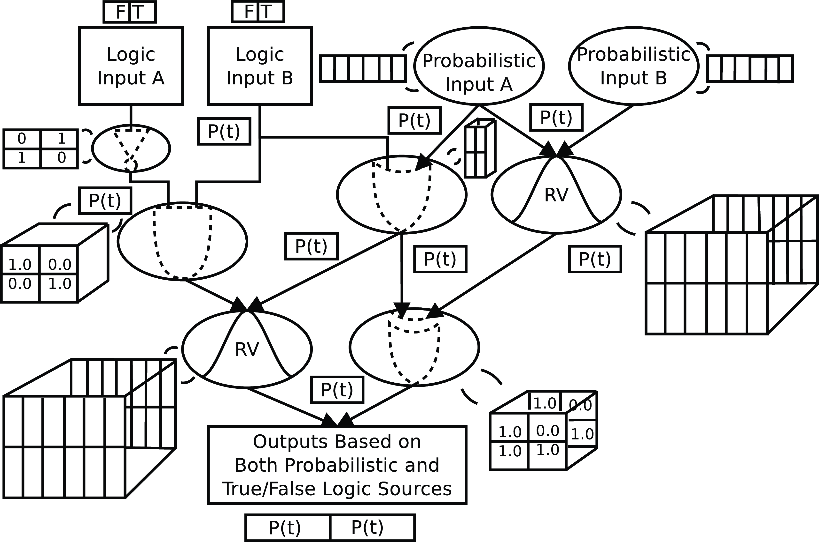
Figure 3. Combined domains of logic. A methodology for combining Boolean and Bayesian logic, in which Boolean operations are subsumed by Bayesian inference and tensors represent Bernoulli random variables (RVs).
3. Boolean logic with Bernoulli random variables
In this section, Bayesian logic is developed that subsumes Boolean logic operations so that they can be combined as described in Section 2. To do this, it is necessary to look at Boolean and Bayesian logic in similar terms – that is, as a logical operation to be performed on one or more variables that follows established logical rules. This novel approach insures that the logic is not only mathematically consistent, but is also consistent in terms of the algorithms and operations that are executed on a computing device to perform it.
The logical rules for probabilistic inference using naive Bayesian logic are well-known [Reference Koller and Friedman23] and are described here using random variables $A$
and
$A$
and $B$
that contain states
$B$
that contain states $a$
and
$a$
and $b$
respectively with
$b$
respectively with $B$
represented as a parent random variable of
$B$
represented as a parent random variable of $A$
, as denoted by membership in the set of parents
$A$
, as denoted by membership in the set of parents $\text{Pa}(A)$
of
$\text{Pa}(A)$
of $A$
, such that the value of
$A$
, such that the value of $A$
depends on
$A$
depends on $B \in \text{Pa}(A)$
as shown in Eq. (1).
$B \in \text{Pa}(A)$
as shown in Eq. (1).
 \begin{equation} \text{P}(A=a) = \sum _{B \in \text{Pa}(A)} \text{P}(A=a | B=b) \text{P}(B=b) \end{equation}
A Bayesian inference operation depends entirely on the conditional probability distribution $\text{P}(A=a | B=b)$
, which for a discrete random variable can be represented as an order
$\text{P}(A=a | B=b)$
, which for a discrete random variable can be represented as an order $(L+1)$
tensor for a random variable dependent on
$(L+1)$
tensor for a random variable dependent on $L$
other random variables [Reference Post32]. The logical operation to be performed can be chosen by selecting this distribution. This tensor [Reference Yilmaz and Cemgil33] is chosen such that the index that represents the inferred distribution (the “output”) is the first index, considered to be the “rows” of a tensor that is represented as a multidimensional array in row-major order.
$L$
other random variables [Reference Post32]. The logical operation to be performed can be chosen by selecting this distribution. This tensor [Reference Yilmaz and Cemgil33] is chosen such that the index that represents the inferred distribution (the “output”) is the first index, considered to be the “rows” of a tensor that is represented as a multidimensional array in row-major order.
In contrast to the number of tensors that could be defined in a Bayesian network, only a few specific operations are defined for Boolean values due to their simplicity. The basic operations commonly used in programming are referred to as logical negation (NOT), logical conjunction (AND), logical disjunction (OR), and exclusive disjunction (XOR). Complementary logic operations are also defined as NAND, NOR, and XNOR, being equivalent to AND, OR, and XOR with a NOT negation operation following the operation. The logical identity operation (which does not change the input) and the logical implication operation (which is non-commutative) are not commonly found in computational logic, but as Boolean operations they can be similarly performed by Bayesian inference, and definitions of these operations are included here for completeness.
Bernoulli random variables are an ideal basis for building a system of probabilistic logic as they assume two states (true and false) depending on a truth probability $p = \text{P}(A=\text{true})$
and a complementary probability
$p = \text{P}(A=\text{true})$
and a complementary probability $q = \text{P}(A=\text{false}) = 1 - p$
. In subscripts, true is denoted by “t” and false is denoted by “f." Bernoulli random variables follow Boolean logic if
$q = \text{P}(A=\text{false}) = 1 - p$
. In subscripts, true is denoted by “t” and false is denoted by “f." Bernoulli random variables follow Boolean logic if $p = 1$
(true) or
$p = 1$
(true) or $q = 1$
(false). We use the letter
$q = 1$
(false). We use the letter $Q$
in the fashion adopted by logical notation to denote the output distribution of an inference operation. In the logic model described here, the conditional probability distribution is represented as
$Q$
in the fashion adopted by logical notation to denote the output distribution of an inference operation. In the logic model described here, the conditional probability distribution is represented as $\text{P}(Q=\text{t}|A,B)$
, with
$\text{P}(Q=\text{t}|A,B)$
, with $Q$
as the Bayesian random variable representing the logic operation and parent variables
$Q$
as the Bayesian random variable representing the logic operation and parent variables $A$
and
$A$
and $B$
representing the inputs as shown in Eq. (2).
$B$
representing the inputs as shown in Eq. (2).
 \begin{equation} \text{P}(Q) = \sum _{a \in A, b \in B} \text{P}(Q|A=a,B=b) \text{P}(A=a) \text{P}(B=b) \end{equation}
As an example calculation, Eq. (3) shows the probability that $Q$
is true as calculated by the total probability (sum) of all system states in which
$Q$
is true as calculated by the total probability (sum) of all system states in which $Q$
is true, from the law of total probability.
$Q$
is true, from the law of total probability.
 \begin{align} \text{P}(Q=\text{t})& = \text{P}(Q=\text{t}|A=\text{t},B=\text{t}) \text{P}(A=\text{t}) \text{P}(B=\text{t}) \nonumber \\[3pt] & \quad +\text{P}(Q=\text{t}|A=\text{t},B=\text{f}) \text{P}(A=\text{t}) \text{P}(B=\text{f}) \nonumber \\[3pt] & \quad +\text{P}(Q=\text{t}|A=\text{f},B=\text{t}) \text{P}(A=\text{f}) \text{P}(B=\text{t}) \nonumber \\[3pt] & \quad +\text{P}(Q=\text{t}|A=\text{f},B=\text{f}) \text{P}(A=\text{f}) \text{P}(B=\text{f}) \end{align}
The conditional probability distribution is represented by a tensor of order $L = 3$
and size
$L = 3$
and size $2 \times 2 \times 2$
for Bernoulli random variables. Representing the conditional probability distribution as a tensor
$2 \times 2 \times 2$
for Bernoulli random variables. Representing the conditional probability distribution as a tensor $P$
, the operation can be defined as
$P$
, the operation can be defined as $P_{ijk} = \text{P}(Q=i|A=j,B=k)$
, where
$P_{ijk} = \text{P}(Q=i|A=j,B=k)$
, where $i \in \{\text{t},\text{f}\}$
,
$i \in \{\text{t},\text{f}\}$
, $j \in \{\text{t},\text{f}\}$
,
$j \in \{\text{t},\text{f}\}$
, $k \in \{\text{t},\text{f}\}$
. Additionally, the probabilities of the parent random variables can be defined in shortened form as
$k \in \{\text{t},\text{f}\}$
. Additionally, the probabilities of the parent random variables can be defined in shortened form as $A_{\text{t}} = \text{P}(A=\text{t})$
,
$A_{\text{t}} = \text{P}(A=\text{t})$
, $A_{\text{f}} = \text{P}(A=\text{f})$
,
$A_{\text{f}} = \text{P}(A=\text{f})$
, $B_{\text{t}} = \text{P}(B=\text{t})$
,
$B_{\text{t}} = \text{P}(B=\text{t})$
, $B_{\text{f}} = \text{P}(B=\text{f})$
. The inference operation is then defined as a tensor inner product with the probability distributions of
$B_{\text{f}} = \text{P}(B=\text{f})$
. The inference operation is then defined as a tensor inner product with the probability distributions of $A$
and
$A$
and $B$
, where the first dimension of the tensor represents the distribution of Q itself as in Eq. (4).
$B$
, where the first dimension of the tensor represents the distribution of Q itself as in Eq. (4).
 \begin{equation} \text{P}(Q) = \begin{bmatrix} P_{\text{ttt}} A_{\text{t}} B_{\text{t}} + P_{\text{tft}} A_{\text{f}} B_{\text{t}} + P_{\text{ttf}} A_{\text{t}} B_{\text{f}} + P_{\text{tff}} A_{\text{f}} B_{\text{f}} \\[5pt] P_{\text{ftt}} A_{\text{t}} B_{\text{t}} + P_{\text{fft}} A_{\text{f}} B_{\text{t}} + P_{\text{ftf}} A_{\text{t}} B_{\text{f}} + P_{\text{fff}} A_{\text{f}} B_{\text{f}} \\ \end{bmatrix} \end{equation}
This leads to the compact representation in Eq. (5) of the inferred probability distribution for Bernoulli random variables.
 \begin{equation} \text{P}(Q) = \begin{bmatrix} \sum _{j,k} P_{\text{t}jk} A_j B_k \\[8pt] \sum _{j,k} P_{\text{f}jk} A_j B_k \end{bmatrix} \end{equation}
Performing a Boolean operation by means of Bayesian inference is now a matter of defining the conditional probability distributions in the form of tensors that produce an equivalent logical output in terms of a Bernoulli distribution.
3.1. Negation and identity
The simplest Boolean logic operation is the unary negation (NOT) operation $\neg A$
, which serves as a good basic reference for comparison between Boolean and Bayesian logic. In the Boolean sense, the output state of this operation is the opposite state of the input.
$\neg A$
, which serves as a good basic reference for comparison between Boolean and Bayesian logic. In the Boolean sense, the output state of this operation is the opposite state of the input.
For the case of a two-valued random variable that can take the state true or false, the conditional probability distribution, represented as a two-dimensional matrix, takes the same form as the truth table for the NOT operation, as shown in Fig. 4. This is because the truth table for the probability $p$
determines the value for
$p$
determines the value for $\text{P}(Q=\text{t}|\ldots )$
, and its complement
$\text{P}(Q=\text{t}|\ldots )$
, and its complement $q$
determines the values for
$q$
determines the values for $\text{P}(Q=\text{f}|\ldots )$
. The conditional probability distribution for a random variable with a single parent is just a matrix that is multiplied in the manner of matrix multiplication with the distribution of the parent random variable to produce the inferred distribution. The conditional probability distribution can also be described as in Eq. (6).
$\text{P}(Q=\text{f}|\ldots )$
. The conditional probability distribution for a random variable with a single parent is just a matrix that is multiplied in the manner of matrix multiplication with the distribution of the parent random variable to produce the inferred distribution. The conditional probability distribution can also be described as in Eq. (6).
 \begin{equation} \begin{cases} \text{P}(Q=\text{f}|A=\text{t}) = 1.0 \\[3pt] \text{P}(Q=\text{t}|A=\text{f}) = 1.0 \\[3pt] \text{P}(Q=\text{t}) = 0.0\, \text{otherwise} \end{cases} \end{equation}
To provide a comparison example, an “identity” conditional random variable (with the operation abbreviated as ID) is created that has the effect of the inferred distribution being identical to the parent random variable, shown in Fig. 5. For a random variable with a single parent $A$
, this distribution takes the form of an identity matrix as the inference operation is again a matrix multiplication.
$A$
, this distribution takes the form of an identity matrix as the inference operation is again a matrix multiplication.
 \begin{equation} \begin{cases} \text{P}(Q=\text{t}|A=\text{t},B=\text{t},\ldots =\text{t}) = 1.0 \\[5pt] \text{P}(Q=\text{t}) = 0.0\, \text{otherwise} \end{cases} \end{equation}
These examples indicate a useful property of the conditional probability distribution for Bernoulli random variables. The negation operation has the effect of reversing the conditional probability distribution along the axis of the values for the random variable as shown in Eq. (8).
 \begin{equation} \text{P}(Q) = \neg \text{P}(A) = 1-\text{P}(A) = 1-[p_{0,0}, p_{1,0}] \end{equation}
Since $p_{1,0} = 1-p_{0,0}$
, the operation of negation on
$p_{1,0} = 1-p_{0,0}$
, the operation of negation on $\text{P}(A)$
is as illustrated in Eq. (9).
$\text{P}(A)$
is as illustrated in Eq. (9).
 \begin{equation} \neg \text{P}(A) = 1-[p_{0,0}, 1-p_{0,0}] = [1-p_{0,0}, p_{0,0}] = [p_{1,0}, p_{0,0}] \end{equation}
Thus, the distribution terms are reversed on negation. Using this rule, the Bernoulli conditional probability distributions can easily be produced that are equivalent to inverted logic operations such as NAND, NOR, and XNOR, from the non-inverted AND, OR, and XOR operations.

Figure 4. Bayesian logical negation (NOT) operation.

Figure 5. Bayesian logical identity (ID) operation.
3.2. Conjunction
The conjunction (AND) operation $A \wedge B \wedge \ldots$
is implemented as a conditional probability distribution by recognizing that the inferred distribution should show a state of true only for the case where all priors are considered to be true. Following the previous example, the indices of the distribution for
$A \wedge B \wedge \ldots$
is implemented as a conditional probability distribution by recognizing that the inferred distribution should show a state of true only for the case where all priors are considered to be true. Following the previous example, the indices of the distribution for $\text{P}(Q=\text{t}|\ldots )$
are set as in Eq. (10).
$\text{P}(Q=\text{t}|\ldots )$
are set as in Eq. (10).
 \begin{equation} \begin{cases} \text{P}(Q=\text{t}|A=\text{t},B=\text{t},\ldots =\text{t}) = 1.0 \\[5pt] \text{P}(Q=\text{t}) = 0.0\, \text{otherwise} \end{cases} \end{equation}
In all cases, $\text{P}(Q=\text{f}|\ldots ) = 1-\text{P}(Q=\text{t}|\ldots )$
. Figure 6 shows the resulting distribution for the case of a two-input AND operation. This method also applies to multiple-input AND operations, as shown by the example of three parent random variables in Fig. 7.
$\text{P}(Q=\text{f}|\ldots ) = 1-\text{P}(Q=\text{t}|\ldots )$
. Figure 6 shows the resulting distribution for the case of a two-input AND operation. This method also applies to multiple-input AND operations, as shown by the example of three parent random variables in Fig. 7.

Figure 6. Bayesian logical conjunction (AND) operation.

Figure 7. Bayesian logical conjunction (AND) operation with three inputs.
3.3. Disjunction
The disjunction (OR) operation $A \vee B \vee \ldots$
is implemented in a complementary fashion to conjunction, by recognizing that the inferred distribution should be true in all cases except for that where all priors are considered to be false, as stated in Eq. (11).
$A \vee B \vee \ldots$
is implemented in a complementary fashion to conjunction, by recognizing that the inferred distribution should be true in all cases except for that where all priors are considered to be false, as stated in Eq. (11).
 \begin{equation} \begin{cases} \text{P}(Q=\text{t}|A=\text{f},B=\text{f},\ldots =\text{f}) = 0.0 \\[5pt] \text{P}(Q=\text{t}) = 1.0 \,\text{otherwise} \end{cases} \end{equation}
The resulting distribution for a two-input OR operation is shown in Fig. 8 and again applies equally to the case of three or more inputs as shown in Fig. 9.

Figure 8. Bayesian logical disjunction (OR) operation.

Figure 9. Bayesian logical disjunction (OR) operation with three inputs.
3.4. Exclusive disjunction
The exclusive disjunction (XOR) operation $A \oplus B \oplus \ldots$
differs from that of OR in that there are two cases in which the inferred distribution should be false, when all priors are considered to be true and when all priors are considered to be false. Equation (12) describes the conditional probability distribution for this operation.
$A \oplus B \oplus \ldots$
differs from that of OR in that there are two cases in which the inferred distribution should be false, when all priors are considered to be true and when all priors are considered to be false. Equation (12) describes the conditional probability distribution for this operation.
 \begin{equation} \begin{cases} \text{P}(Q=\text{t}|A=\text{t},B=\text{t},\ldots =\text{t}) = 0.0 \\[3pt] \text{P}(Q=\text{t}|A=\text{f},B=\text{f},\ldots =\text{f}) = 0.0 \\[3pt] \text{P}(Q=\text{t}) = 1.0\, \text{otherwise} \end{cases} \end{equation}
The resulting distribution for a two-input XOR operation is shown in Fig. 10 and again applies equally to the case of three or more inputs as shown in Fig. 11.

Figure 10. Bayesian logical exclusive disjunction (XOR) operation.

Figure 11. Bayesian logical exclusive disjunction (XOR) operation with three inputs.
3.5. Material implication
Material implication (which is abbreviated here as IMP) differs from the logical operations above that are used for computational logic in that the special cases for a multiple-input operation are not simply those of all-true or all-false. This means that the operation is not commutative – the ordering and identity of the priors matters, and one input is distinct as the hypothesis. For the case of implication ( $A \rightarrow B$
), Eq. (13) provides the conditional probability distribution.
$A \rightarrow B$
), Eq. (13) provides the conditional probability distribution.
 \begin{equation} \begin{cases} \text{P}(Q=\text{t}|A=\text{t},B=\text{f}) = 0.0 \\[4pt] \text{P}(Q=\text{t}) = 1.0 \,\text{otherwise} \end{cases} \end{equation}
Figure 12 shows the distribution that results. The reverse case of converse implication (CIMP) $A \leftarrow B$
is provided by simply setting
$A \leftarrow B$
is provided by simply setting $\text{P}(Q=\text{t}|A=\text{t},B=\text{f}) = 0.0$
in Eq. (13).
$\text{P}(Q=\text{t}|A=\text{t},B=\text{f}) = 0.0$
in Eq. (13).

Figure 12. Bayesian logical implication (IMP) operation.
Although the Boolean implication operation is not defined for multiple inputs, the extension of Eq. (13) to multiple variables is proposed in this methodology as an appropriate definition of multiple-input implication. This naturally produces the operation $A \rightarrow (B \vee C \vee \ldots )$
in which all input random variables other than the one serving as hypothesis are treated as a single disjunction. By defining the operation as false only if
$A \rightarrow (B \vee C \vee \ldots )$
in which all input random variables other than the one serving as hypothesis are treated as a single disjunction. By defining the operation as false only if $A$
is true and all other variables are false, only one tensor entry for
$A$
is true and all other variables are false, only one tensor entry for $\text{P}(Q=\text{t}|\ldots )$
needs to be defined as false, and the conditional probability distribution takes the form of Eq. (14).
$\text{P}(Q=\text{t}|\ldots )$
needs to be defined as false, and the conditional probability distribution takes the form of Eq. (14).
 \begin{equation} \begin{cases} \text{P}(Q=\text{t}|A=\text{t},B=\text{f},\ldots =\text{f}) = 0.0 \\[4pt] \text{P}(Q=\text{t}) = 1.0 \,\text{otherwise} \end{cases} \end{equation}
Using this new proposed formulation, the distribution shown in Fig. 13 is produced. Any parent random variable (the first parent input $A$
is suggested here for convenience) can be selected as the implication input for this operation, which when true will require at least one of the other inputs to also be true for the operation output to be true. The converse implication operation for multiple variables ceases to have distinct meaning in this interpretation as it is simply the use of a different input variable. The negation of implication however (abbreviated here as NIMP) still a distinct operation that can again be accomplished by reversing the conditional probability distribution as described above.
$A$
is suggested here for convenience) can be selected as the implication input for this operation, which when true will require at least one of the other inputs to also be true for the operation output to be true. The converse implication operation for multiple variables ceases to have distinct meaning in this interpretation as it is simply the use of a different input variable. The negation of implication however (abbreviated here as NIMP) still a distinct operation that can again be accomplished by reversing the conditional probability distribution as described above.

Figure 13. Bayesian logical implication (IMP) operation extended to three inputs as proposed by $A \rightarrow (B \vee C \vee \ldots )$
.
$A \rightarrow (B \vee C \vee \ldots )$
.
While implementing the multiple-input IMP operation as $A \rightarrow (B \wedge C \wedge \ldots )$
is possible, in which all input random variables other than the hypothesis are treated as a single conjunction, it is both less efficient to generate and less useful in the sense that the output is identical to the hypothesis in all cases other than when all variables are true and thus requires setting conditional probabilities separately for
$A \rightarrow (B \wedge C \wedge \ldots )$
is possible, in which all input random variables other than the hypothesis are treated as a single conjunction, it is both less efficient to generate and less useful in the sense that the output is identical to the hypothesis in all cases other than when all variables are true and thus requires setting conditional probabilities separately for $L$
parents rather than setting a single case.
$L$
parents rather than setting a single case.
Having defined Boolean operations in terms of Bayesian inference, more detail in their properties can now be explored with respect to Boolean logic systems that can propagate probabilistic information.
4. Hybrid probabilistic logic
In this section, the ability for Bayesian logic and Boolean logic based on the logic described previously to coexist side by side is examined in the interest of creating a system where uncertainty can be propagated even in elements that are not Boolean. Until now, only “definite” Bernoulli random variables that follow the function of Boolean logic have been considered. The effects of introducing priors with uncertainty (probability values other than 1.0 and 0.0) are now considered in systems with definite probability distributions as described above, and also the effect of combining uncertain states with a different number of inputs to an operation.
4.1. Product forms
The single-input identity and negation (NOT) operations are simple in their application, so instead multiple-input operations with more than one parent random variable are considered here. To begin with, consider the example of a two-input logical conjunction (AND) operation. Applying the expanded tensor inner product of Eq. (4) to the AND operation tensor constructed in Eq. (10) results in the expansion as follows, here shown with $\text{P}(Q=\text{t}|A,B)$
on the “top” of column vectors and
$\text{P}(Q=\text{t}|A,B)$
on the “top” of column vectors and $\text{P}(Q=\text{f}|A,B)$
on the “bottom” of Eq. (15).
$\text{P}(Q=\text{f}|A,B)$
on the “bottom” of Eq. (15).
 \begin{align} \text{P}(Q_{\text{AND}}|A,B){} & = \left[\begin{array}{c} (1.0) A_{\text{t}} B_{\text{t}} + (0.0) A_{\text{f}} B_{\text{t}} + (0.0) A_{\text{t}} B_{\text{f}} + (0.0) A_{\text{f}} B_{\text{f}} \\[5pt] (0.0) A_{\text{t}} B_{\text{t}} + (1.0) A_{\text{f}} B_{\text{t}} + (1.0) A_{\text{t}} B_{\text{f}} + (1.0) A_{\text{f}} B_{\text{f}} \\[5pt] \end{array}\right] \nonumber \\[5pt] & = \left[\begin{array}{c} A_{\text{t}} B_{\text{t}} \\[5pt] A_{\text{f}} B_{\text{t}} + A_{\text{t}} B_{\text{f}} + A_{\text{f}} B_{\text{f}} \\[5pt] \end{array}\right] \end{align}
The same pattern can be seen in the expansion of the logical disjunction (OR) operation constructed in Eq. (11) that is given in Eq. (16), exclusive disjunction (XOR) operation constructed in Eq. (12) that is given in Eq. (17), and logical implication (IMP) operation constructed in Eq. (13) that is given in Eq. (18).
 \begin{eqnarray} \text{P}(Q_{\text{OR}}|A,B){}&=& \begin{bmatrix} (1.0) A_{\text{t}} B_{\text{t}} + (1.0) A_{\text{f}} B_{\text{t}} + (1.0) A_{\text{t}} B_{\text{f}} + (0.0) A_{\text{f}} B_{\text{f}} \\[5pt] (0.0) A_{\text{t}} B_{\text{t}} + (0.0) A_{\text{f}} B_{\text{t}} + (0.0) A_{\text{t}} B_{\text{f}} + (1.0) A_{\text{f}} B_{\text{f}} \\[5pt] \end{bmatrix} \nonumber \\[5pt] &=&\begin{bmatrix} A_{\text{t}} B_{\text{t}} + A_{\text{f}} B_{\text{t}} + A_{\text{t}} B_{\text{f}} \\[5pt] A_{\text{f}} B_{\text{f}} \\[5pt] \end{bmatrix} \end{eqnarray}
 \begin{eqnarray} \text{P}(Q_{\text{XOR}}|A,B){}&= & \begin{bmatrix} (0.0) A_{\text{t}} B_{\text{t}} + (1.0) A_{\text{f}} B_{\text{t}} + (1.0) A_{\text{t}} B_{\text{f}} + (0.0) A_{\text{f}} B_{\text{f}} \\[5pt] (1.0) A_{\text{t}} B_{\text{t}} + (0.0) A_{\text{f}} B_{\text{t}} + (0.0) A_{\text{t}} B_{\text{f}} + (1.0) A_{\text{f}} B_{\text{f}} \\[5pt] \end{bmatrix} \nonumber \\[5pt] &=&\begin{bmatrix} A_{\text{f}} B_{\text{t}} + A_{\text{t}} B_{\text{f}} \\[5pt] A_{\text{t}} B_{\text{t}} + A_{\text{f}} B_{\text{f}} \\[5pt] \end{bmatrix} \end{eqnarray}
 \begin{eqnarray} \text{P}(Q_{\text{IMP}}|A,B){}&= & \begin{bmatrix} (1.0) A_{\text{t}} B_{\text{t}} + (0.0) A_{\text{f}} B_{\text{t}} + (1.0) A_{\text{t}} B_{\text{f}} + (1.0) A_{\text{f}} B_{\text{f}} \\[5pt] (0.0) A_{\text{t}} B_{\text{t}} + (1.0) A_{\text{f}} B_{\text{t}} + (0.0) A_{\text{t}} B_{\text{f}} + (0.0) A_{\text{f}} B_{\text{f}} \\[5pt] \end{bmatrix} \nonumber \\[5pt] &=&\begin{bmatrix} A_{\text{t}} B_{\text{t}} + A_{\text{f}} B_{\text{t}} + A_{\text{f}} B_{\text{f}} \\[5pt] A_{\text{t}} B_{\text{f}} \\[5pt] \end{bmatrix} \end{eqnarray}
This expansion demonstrates how probabilistic logic with Bernoulli random variables can differ from Boolean logic. It is clear that due to the imposed Boolean logic structure of all conditional probability distribution terms being either $1.0$
or
$1.0$
or $0.0$
, and the probabilities along the random variable distribution summing to
$0.0$
, and the probabilities along the random variable distribution summing to $1.0$
in all cases, each combination of input product
$1.0$
in all cases, each combination of input product $AB$
terms appears only in one place in the inferred distribution. Note that a negation (NAND, NOR, XNOR) has the effect already explained of reversing the probabilities of the inferred distribution.
$AB$
terms appears only in one place in the inferred distribution. Note that a negation (NAND, NOR, XNOR) has the effect already explained of reversing the probabilities of the inferred distribution.
This leads to a sum-of-products expression for each of the Boolean-derived probabilistic logic operations that can be used as an efficient way to produce these logic operations numerically and makes the result of a hybrid logic calculation clear to see. This sum-of-products expression is equivalent to a Boolean sum-of-products expression, indicating that if a set of purely Boolean values $\{1.0, 0.0\}$
are used as inputs, only one of the product terms will result in a probability of
$\{1.0, 0.0\}$
are used as inputs, only one of the product terms will result in a probability of $\mathrm{P}(Q=\text{t}|A,B) = 1.0$
. Due to the conceptual parallel with the Boolean sum-of-products form, these products within the sum are also referred to as “minterms," and validate that the proposed methodology produces the same results as an equivalent Boolean logic system.
$\mathrm{P}(Q=\text{t}|A,B) = 1.0$
. Due to the conceptual parallel with the Boolean sum-of-products form, these products within the sum are also referred to as “minterms," and validate that the proposed methodology produces the same results as an equivalent Boolean logic system.
Of much greater interest is the result if probabilities that do not indicate certainty and lie in the interval $[0, 1]$
are used, for input random variables of the form
$[0, 1]$
are used, for input random variables of the form $\mathrm{P}(A=t) = A_{\text{t}} = [0.0, 1.0]$
,
$\mathrm{P}(A=t) = A_{\text{t}} = [0.0, 1.0]$
, $\text{P}(A=f) = A_{\text{f}} = 1.0 - A_{\text{t}}$
. If either
$\text{P}(A=f) = A_{\text{f}} = 1.0 - A_{\text{t}}$
. If either $A_{\text{t}} = 0$
or
$A_{\text{t}} = 0$
or $B_{\text{t}} = 0$
in an AND operation, it is clear from the minterms that
$B_{\text{t}} = 0$
in an AND operation, it is clear from the minterms that $A_{\text{t}} B_{\text{t}}$
will be
$A_{\text{t}} B_{\text{t}}$
will be $0$
and the output will be definite with
$0$
and the output will be definite with $\text{P}(Q_{\text{AND}}=\text{t}|A,B) = 0$
, which reflects the removal of uncertainty by the ultimate dependence on both inputs.
$\text{P}(Q_{\text{AND}}=\text{t}|A,B) = 0$
, which reflects the removal of uncertainty by the ultimate dependence on both inputs.
Similarly, in the OR operation, if either $A_{\text{t}} = 1$
or
$A_{\text{t}} = 1$
or $B_{\text{t}} = 1$
, it is clear from the minterms that
$B_{\text{t}} = 1$
, it is clear from the minterms that $A_{\text{f}} B_{\text{f}}$
will be
$A_{\text{f}} B_{\text{f}}$
will be $0$
and the output will be definite with
$0$
and the output will be definite with $\text{P}(Q_{\text{OR}}=\text{t}|A,B) = 1$
.
$\text{P}(Q_{\text{OR}}=\text{t}|A,B) = 1$
.
Logical implication as presented in this work is similar to AND with one minterm determining the probability that the result is false, but indicates the specific values of inputs that will produce $\text{P}(Q_{\text{IMP}}=\text{t}|A,B) = 0$
, and definite truth is implied if any of these input values are
$\text{P}(Q_{\text{IMP}}=\text{t}|A,B) = 0$
, and definite truth is implied if any of these input values are $0$
, and uncertainty if not.
$0$
, and uncertainty if not.
An XOR operation is different in that there are two minterms for each state, and given the definite $A_{\text{t}} = 0$
, then
$A_{\text{t}} = 0$
, then $\text{P}(Q_{\text{XOR}}=\text{t}|A,B) = B_{\text{t}}$
, while
$\text{P}(Q_{\text{XOR}}=\text{t}|A,B) = B_{\text{t}}$
, while $A_{\text{t}} = 1$
, results in
$A_{\text{t}} = 1$
, results in $\text{P}(Q_{\text{XOR}}=\text{t}|A,B) = B_{\text{f}}$
. Both
$\text{P}(Q_{\text{XOR}}=\text{t}|A,B) = B_{\text{f}}$
. Both $A$
and
$A$
and $B$
must be definite to produce a definite output in XOR, and like the pure Boolean operation, it effectively serves as a selectable negation operation when one input is definite while uncertainty is passed through the other. These minterms clearly indicate how both certainty and uncertainty are propagated together through hybrid logic operations.
$B$
must be definite to produce a definite output in XOR, and like the pure Boolean operation, it effectively serves as a selectable negation operation when one input is definite while uncertainty is passed through the other. These minterms clearly indicate how both certainty and uncertainty are propagated together through hybrid logic operations.
In summary, the different logic operations as proposed in this methodology provide different “tolerances” to uncertainty in one variable with other variables being definite, as indicated by analysis of Eqs. (15)–(18).
-
AND definite false if one input is definite false, otherwise propagates uncertainty in other inputs
-
OR definite true if one input is definite true, otherwise propagates uncertainty in other inputs
-
XOR not definite unless all inputs definite; one definite input being true will invert the other with two inputs
-
IMP definite false if hypothesis input is definite true and all others false, otherwise propagates other inputs
4.2. Number of inputs
The number of inputs $L$
as parent random variables to the operation is highly relevant to the resulting inferred distribution. In the case of AND, OR, and implication operations, only one minterm will appear in one of the inferred distribution state probabilities (either for true or for false) and for an XOR operation two minterms, regardless of the number of inputs. The remaining terms appear in the opposite state probability. As Bernoulli random variables are restricted to two states, this can be seen to heavily bias the “output” inferred distribution of the operation in favour of the state in which more terms appear.
$L$
as parent random variables to the operation is highly relevant to the resulting inferred distribution. In the case of AND, OR, and implication operations, only one minterm will appear in one of the inferred distribution state probabilities (either for true or for false) and for an XOR operation two minterms, regardless of the number of inputs. The remaining terms appear in the opposite state probability. As Bernoulli random variables are restricted to two states, this can be seen to heavily bias the “output” inferred distribution of the operation in favour of the state in which more terms appear.
This behaviour is a consequence of the uncertainty that is built into the concept of a random variable, as seen in the context of a logical operation. A Boolean operation with $L$
independent and uncertain inputs that all have a probability
$L$
independent and uncertain inputs that all have a probability $p$
of state true and probability
$p$
of state true and probability $q=1-p$
of state false can be modelled by a binomial distribution. In the case of a Boolean AND operation, the probability of the operation resulting in true is
$q=1-p$
of state false can be modelled by a binomial distribution. In the case of a Boolean AND operation, the probability of the operation resulting in true is $p^L$
, while in the case of a Boolean OR operation, the probability of the operation resulting in true is
$p^L$
, while in the case of a Boolean OR operation, the probability of the operation resulting in true is $1-q^L$
, which typically is a larger value for large
$1-q^L$
, which typically is a larger value for large $L$
. As the XOR operation has two terms in which the result is false, the probability is
$L$
. As the XOR operation has two terms in which the result is false, the probability is $p^L + q^L$
in this case. Even in the case of entirely uncertain input state probabilities
$p^L + q^L$
in this case. Even in the case of entirely uncertain input state probabilities $p=0.5$
and
$p=0.5$
and $q=0.5$
, the output will be biased depending on the type of logical operation to a degree proportional to the number of inputs.
$q=0.5$
, the output will be biased depending on the type of logical operation to a degree proportional to the number of inputs.
Since the probability distributions of parent random variables (inputs) to a logical operation will vary, a more general description of the truth probability of the inferred distribution (output) $\text{P}(Q=\text{true})$
is preferred and takes the form of a product of the truth probability of the parent random variables
$\text{P}(Q=\text{true})$
is preferred and takes the form of a product of the truth probability of the parent random variables $X_l$
in
$X_l$
in $\text{Pa}(Q)$
to the logical operation random variable
$\text{Pa}(Q)$
to the logical operation random variable $Q$
. For clarity of notation, the
$Q$
. For clarity of notation, the $L$
probabilities of truth for each parent random variable in
$L$
probabilities of truth for each parent random variable in $\text{Pa}(Q)$
are denoted as
$\text{Pa}(Q)$
are denoted as $p_l$
and the corresponding probabilities of falsity are denoted as
$p_l$
and the corresponding probabilities of falsity are denoted as $q_l = 1 - p_l$
as stated in Eqs. (19) and 20.
$q_l = 1 - p_l$
as stated in Eqs. (19) and 20.
 \begin{eqnarray} p_l = \text{P}(X_l=\text{true}), X_l \in \text{Pa}(Q) \end{eqnarray}
 \begin{eqnarray} q_l = \text{P}(X_l=\text{false}) = 1 - p_l, X_l \in \text{Pa}(Q) \end{eqnarray}
Table I provides a summary of the probability of these truth probabilities for the operations discussed here as a product of input truth probabilities from $\text{Pa}(Q)$
. If all these probabilities are identical and represented by
$\text{Pa}(Q)$
. If all these probabilities are identical and represented by $p_l$
, the probability of truth can be calculated with respect to
$p_l$
, the probability of truth can be calculated with respect to $L$
, as on the right side of this table. As it is not commutative, the logical implication operation (IMP) that is here defined as
$L$
, as on the right side of this table. As it is not commutative, the logical implication operation (IMP) that is here defined as $A \rightarrow (B \vee C \vee \ldots )$
for multiple inputs and its negation (NIMP) must specify one variable
$A \rightarrow (B \vee C \vee \ldots )$
for multiple inputs and its negation (NIMP) must specify one variable $A$
to be the hypothesis, and this variable is considered here for simplicity to be the first indexed parent at
$A$
to be the hypothesis, and this variable is considered here for simplicity to be the first indexed parent at $l = 1$
.
$l = 1$
.
Table I. The dependence of inferred probability of truth $\text{P}(Q=\text{true})$
on the number of parent inputs
$\text{P}(Q=\text{true})$
on the number of parent inputs $\text{Pa}(Q)$
for probabilistic logic operations. Assuming that all
$\text{Pa}(Q)$
for probabilistic logic operations. Assuming that all $L$
probabilities of truth
$L$
probabilities of truth $p_l = 1-q_l$
in
$p_l = 1-q_l$
in $\text{Pa}(Q)$
are the same, the scaling of
$\text{Pa}(Q)$
are the same, the scaling of $p$
by the number of inputs
$p$
by the number of inputs $L$
is calculated.
$L$
is calculated.

Note: For IMP and CIMP, the input at l = 1 is the hypothesis.
Although this scaling is a significant factor in the design of logical programmes that involve uncertainty, it is important to note that if the inputs (probability distributions of parent random variables) are traditional Boolean quantities and therefore certain in state, then $p$
must be either
$p$
must be either $0.0$
or
$0.0$
or $1.0$
. In this case, the minterms in Eqs. (15)–(18) will also reduce to either
$1.0$
. In this case, the minterms in Eqs. (15)–(18) will also reduce to either $0.0$
or
$0.0$
or $1.0$
, and the certainty of state implied in Boolean logic will continue to propagate throughout the system until a probability value
$1.0$
, and the certainty of state implied in Boolean logic will continue to propagate throughout the system until a probability value $1.0 \gt p \gt 0.0$
is introduced into a variable, at which point uncertainty will cause the number of parent variables to affect the probability distribution. This proves that the certainty of Boolean logic and consequential invariance with number of inputs is retained in the proposed methodology, while allowing uncertainty to act on the system in a means consistent with Bayesian inference.
$1.0 \gt p \gt 0.0$
is introduced into a variable, at which point uncertainty will cause the number of parent variables to affect the probability distribution. This proves that the certainty of Boolean logic and consequential invariance with number of inputs is retained in the proposed methodology, while allowing uncertainty to act on the system in a means consistent with Bayesian inference.
5. Robotic programming
In this section, a hybrid Bayesian and Boolean logic programme for mobile robot control is tested based on the described methodology. To illustrate how Boolean logic and Bayesian logic can coexist by the use of Bernoulli random variables, elements are introduced that not only are purely logical but also depend on uncertainties inherited from the environment and from the internal design of the robot. The use of hybrid logic also facilitates operations such as probabilistic sensor fusion that would otherwise be complex to programme in traditional computing.
5.1. Programming structure
The framework for programming Bayesian inference as described here makes use of arithmetic operations in fixed-point arithmetic for high efficiency and C structures with the following members that realize Bayesian network nodes following the methodology described above [Reference Post32]:
name: A unique name string for identification of the node
numParents: The integer number $L$
of node parents
$L$
of node parentsparent: An ordered array of integer node numbers indicating the parents of the node
numVals: The integer number of states or discrete node distribution size (
$N$
)distSize: The total size in words of the order
$L+1$
distribution tensorconditionals: A fixed-point array for the size
$N$
inferred (conditional) distributiondistributions: A fixed-point array for the order
$L+1$
distribution tensordistFunction: A pointer to a single-input single-output fixed-point function used to populate the probability distribution if a special operation is needed (e.g., a continuous distribution function or a connection to a sensor or actuator)


Linear array indexing with an array declared with fixed size is used to store the list of node structures and the order $L+1$
tensor that represents the conditional probability distribution, and operations are bounds-checked to prevent pointer arithmetic errors. The tensor is indexed in row-major order, with the first dimension of the tensor sized to represent the internal probability distribution of the Bayesian node, and subsequent dimensions sized to represent the distributions of sizes
$L+1$
tensor that represents the conditional probability distribution, and operations are bounds-checked to prevent pointer arithmetic errors. The tensor is indexed in row-major order, with the first dimension of the tensor sized to represent the internal probability distribution of the Bayesian node, and subsequent dimensions sized to represent the distributions of sizes $M_l$
of the parents
$M_l$
of the parents $l = 1 \ldots L$
. The index
$l = 1 \ldots L$
. The index $i$
into the linear array is calculated for each access of the tensor.
$i$
into the linear array is calculated for each access of the tensor.
 \begin{align}{c} i & = m_1 + m_2 M_1 + m_3 M_2 M_1 + \ldots + m_{L+1} \prod _{l=1}^L M_l \nonumber\\[4pt]&= \sum _{n=1}^{L+1} \left ( m_n \prod _{l=1}^{n-1} M_l \right ). \end{align}
This requires an array of total size $N \prod _{l=1}^L M_l$
. For subsuming Boolean logic using Bernoulli random variables as in the proposed methodology,
$N \prod _{l=1}^L M_l$
. For subsuming Boolean logic using Bernoulli random variables as in the proposed methodology, $M_l = 2$
in all cases except when a parent node is not a Bernoulli random variable, but instead is a general random variable with more than two states (shown in Eq. 21).
$M_l = 2$
in all cases except when a parent node is not a Bernoulli random variable, but instead is a general random variable with more than two states (shown in Eq. 21).
The advantages of programming behaviours in the manner of a flexible Bayesian network include that the programme is robust against unexpected system states and logical faults (such as division by zero or undesired negative results) as all calculation is done entirely by tensor-based multiplication operations on a field with known size of defined random variable states. The behavioural programme can also be changed quickly and easily by changing the tensor values that represent the conditional probability distribution of the nodes, as well as the structure of the network itself, which makes it practical to change behavioural programmes and implement machine learning methods that operate on probabilistic data.
5.2. Robot behaviour logic programme
To illustrate how the use of hybrid Boolean and Bayesian logic can process sensor information and produce system behaviours, I created a simulation scenario within the CoppeliaSim 4.2.0 robotics simulator environment. The scene included a simple differential drive mobile robot with multiple sensor inputs, an obstacle, and a goal location with a beacon that the robot can sense. I implemented the logic programme for navigation using the C programming language. The scenario and starting position of the robot are illustrated in Fig. 14. A mobile robot with a sensor that can identify the approximate direction of a target beacon must travel to the target and also avoid an obstacle that lies between the robot and the target. The robot must identify from sensor signals how to turn so as to avoid the obstacle while travelling in the direction of the target. As the focus of this analysis is to exemplify a hybrid logic programme and compare Boolean and hybrid logic results based on the proposed methodology rather than to design a useable hybrid logic control system, no closed-loop control or robotic movement model is used.

Figure 14. The scenario for the analysis of robotic navigational sensor processing. A mobile robot with sensor arcs $\{L, FL, F, FR, R\}$
must reach a target that is sensed by means of a beacon signal with some uncertainty, while avoiding an obstacle in the way that is sensed by rangefinders and a physical collision detector. The outline arrows show the movement of the robot in the time period considered.
$\{L, FL, F, FR, R\}$
must reach a target that is sensed by means of a beacon signal with some uncertainty, while avoiding an obstacle in the way that is sensed by rangefinders and a physical collision detector. The outline arrows show the movement of the robot in the time period considered.

Figure 15. The navigation programme for mobile robot control, as a network of Boolean logic gates. The decision for forward (“Fwd”) is an OR operation, speed (“Spd”) is an AND operation, and direction control (“Dir”) is a set of AND gates representing the desired direction of movement, turning.
Three kinds of external sensors are used. First, an obstacle collision sensor produces a Boolean output of true to indicate a collision has occurred. Obstacle avoidance is implemented using obstacle range sensors with an infrared range measurement model to detect obstacles and produce a probability distribution that indicates the relative probability of obstacle presence across direction states. Navigation is driven by a direction sensor that is modelled on a directional infrared beacon, that provides a Gaussian probability distribution over states of the directional movement. Boolean logic is used to determine the most appropriate action to take based on the sensor input in the same manner that logical rules are used to govern many types of robotic movement. However, when they are realized as Bayesian nodes, they propagate the uncertainty estimates in the sensors through the entire system so that it can be used as part of further decision-making processes. The actuators for the robot are modelled after a typical differential drive robot, and consist of two motors opposite each other that produce forward speed when rotating in the same direction, and turning based on the difference between their rotation speeds. The actuators of the robot are only the left and right motors, which can only be switched forward or reverse using Boolean logic, but using inference can be scaled in speed proportional to the probability value of the relevant random variables for forward and reverse movement, assuming higher certainty should result in higher movement speed.
The Boolean logic programme is written in C the language using the software framework described in [Reference Post32] with the logic layout shown in Fig. 15. This system is based on sensor inputs to drive behaviour with Boolean two-state information in traditional fashion. While it is very simplistic compared to most practical robotic control programmes, it is used here only for the purpose of comparing the differences between Boolean and hybrid Bayesian logic. The sensory responses provided by Boolean logic are compared to those of a system that uses the proposed methodology to replace Boolean logic with Bayesian inference for the same logic structure and operations, as shown in Fig. 16. The implemented programme is shown exported directly as a Bayesian network in Fig. 17. All are created using the common framework detailed above so that a single programming methodology is followed throughout. All decisions are implemented as inference operations into linked random variables, each with posterior probability values for the states {false, true}. The conditional probability distributions are set for each type of logic operation as described in Eq. (6) and Eqs. (10)–(14), and the process of inference is done as in Eq. (1) using the tensor indexing from Eq. (21). To compare the use of purely Boolean logic to Bayesian in an appropriate context, it is assumed that a probability $p \gt = 0.5, q \lt = 0.5$
corresponds to a logic true; otherwise, a logic false is propagated. Therefore, if a state of the target sensor, visual obstacle detection, or direction estimate are above
$p \gt = 0.5, q \lt = 0.5$
corresponds to a logic true; otherwise, a logic false is propagated. Therefore, if a state of the target sensor, visual obstacle detection, or direction estimate are above $0.5$
, it is considered in the Boolean interpretation to be true. Only the probability of truth
$0.5$
, it is considered in the Boolean interpretation to be true. Only the probability of truth $p$
is plotted against time in time steps
$p$
is plotted against time in time steps $t$
in Figs. 19–26 as the complementary state
$t$
in Figs. 19–26 as the complementary state $q = 1 - p$
is implied at all times. The programme is run in separate test cases using Boolean logic and then using hybrid Bayesian logic. In both cases, the programme runs its main loop at a frequency of
$q = 1 - p$
is implied at all times. The programme is run in separate test cases using Boolean logic and then using hybrid Bayesian logic. In both cases, the programme runs its main loop at a frequency of $10$
Hz, which means that the states of all logic gates and random variables on the robot are updated every “time step” of
$10$
Hz, which means that the states of all logic gates and random variables on the robot are updated every “time step” of $0.1$
s. Comparing operation under Boolean logic to that under Bayesian, the robot follows a similar trajectory, but actions are performed differently due to the use of uncertainty information (for example, in setting motor speeds to intermediate values) leading to a timing difference between runs (the robot reaches the obstacle faster in the Boolean case but takes more time to avoid it). Example images indicating the path that the robot takes by illustration of positions at the associated time step numbers are shown in Fig. 18.
$0.1$
s. Comparing operation under Boolean logic to that under Bayesian, the robot follows a similar trajectory, but actions are performed differently due to the use of uncertainty information (for example, in setting motor speeds to intermediate values) leading to a timing difference between runs (the robot reaches the obstacle faster in the Boolean case but takes more time to avoid it). Example images indicating the path that the robot takes by illustration of positions at the associated time step numbers are shown in Fig. 18.

Figure 16. The navigation programme for mobile robot control using the proposed methodology for Boolean logic within a Bayesian network. The same number of elements is used for behaviour determination, but inputs and outputs are provided as separate random variables for each state, and probability values are propagated.

Figure 17. The navigation programme for mobile robot control. Fully implemented using the proposed methodology, in the form of a Bayesian network.

Figure 18. The positions of the robot during its path through the simulation. Positions illustrated are at time step numbers $0$
(a),
$0$
(a), $160$
(b),
$160$
(b), $280$
(c),
$280$
(c), $380$
(d),
$380$
(d), $470$
(e), and
$470$
(e), and $580$
(f).
$580$
(f).
5.3. Sensory inputs
Information from direction-dependent sensors is split into five directional components to approximate angular position as Boolean variables. The facing direction $\theta$
that the sensed quantity refers to in the body frame of the robot is denoted by
$\theta$
that the sensed quantity refers to in the body frame of the robot is denoted by $F$
(front),
$F$
(front), $FL$
(front-left),
$FL$
(front-left), $FR$
(front-right),
$FR$
(front-right), $L$
(left), and
$L$
(left), and $R$
(right), such that
$R$
(right), such that $\theta \in \{L, FL, F, FR, R\}$
.
$\theta \in \{L, FL, F, FR, R\}$
.
In a purely Bayesian or probabilistic inference approach, this information can be stored as a single random variable with five states, using a tensor of order 6 to store the conditional probability distribution. However, as the aim of this work is to show how probabilistic inference can operate as Boolean two-state logic, these states are actually implemented as separate Bernoulli random variables as indicated above. It should be noted that in this system, the use of multiple Bernoulli probability values in a set of states such as “direction” is not conceptually the same as a single random variable with multiple states, because the total of all probabilities for the directions $F$
,
$F$
, $FL$
,
$FL$
, $FR$
,
$FR$
, $L$
, and
$L$
, and $R$
does not necessarily sum to
$R$
does not necessarily sum to $1$
. Instead,
$1$
. Instead, $p + q = 1$
for two states. In comparison to using a single random variable as above, the probability
$p + q = 1$
for two states. In comparison to using a single random variable as above, the probability $p$
of each sensor direction can be independently in the range
$p$
of each sensor direction can be independently in the range $[0\ldots 1]$
without being normalized with respect to the probabilities of other sensor directions. Therefore, the numerical outputs of the sensor array will be different and it is important to consider this distinction with respect to how the sensor programming of the robot is interpreted logically.
$[0\ldots 1]$
without being normalized with respect to the probabilities of other sensor directions. Therefore, the numerical outputs of the sensor array will be different and it is important to consider this distinction with respect to how the sensor programming of the robot is interpreted logically.
The navigation target is named “Target” and is assumed to contain a directional beacon that the robot can sense to serve as a reference point for navigation. The target direction sensing model assumes that the probability distribution of the sensor follows a discretized Gaussian “normal” distribution $\mathcal{N}(\mu,\sigma ^2)$
, and it is assumed that the mean of the distribution is located at the angle to target
$\mathcal{N}(\mu,\sigma ^2)$
, and it is assumed that the mean of the distribution is located at the angle to target $\mu = \theta _T$
and that the direction sense grows stronger and more directional the closer the robot is to the sensor, such that the standard deviation
$\mu = \theta _T$
and that the direction sense grows stronger and more directional the closer the robot is to the sensor, such that the standard deviation $\sigma = r_T/2$
decreases with range to target
$\sigma = r_T/2$
decreases with range to target $r_T$
. The sensor directional components are located at angles
$r_T$
. The sensor directional components are located at angles $\theta = [{-}\pi/3, -\pi/6, 0, \pi/6, \pi/3]$
and sample the probability distribution of the beacon at these values. A Boolean logic direction estimate to the target is obtained by the probability of the target being greater than
$\theta = [{-}\pi/3, -\pi/6, 0, \pi/6, \pi/3]$
and sample the probability distribution of the beacon at these values. A Boolean logic direction estimate to the target is obtained by the probability of the target being greater than $0.3$
$0.3$ $(p_{\theta } \gt 0.3)$
in these directions. More than one sensing direction can be true at a time.
$(p_{\theta } \gt 0.3)$
in these directions. More than one sensing direction can be true at a time.
The values for the “Target” nodes as the robot navigates through the simulation are shown in Fig. 19. In the Boolean logic case, logic values for the forward directions overlap due to the spread of the target distribution and can be seen to cycle rapidly as the robot turns left and right in small increments to track the location of the beacon in the interval between $t=[80,180]$
time steps while the robot is turning towards the target. This rapid cycling behaviour is seen often in Boolean logic cases where discrete feedback thresholds are used. In the hybrid Bayesian logic case, a gradual change in probabilities occurs as the robot tracks the target. The probability values are seen to diverge as the robot gets closer to the target and the spread of the Gaussian sensor distribution decreases, making it clearer over time which direction dominates. This allows the robot to quantify directional probabilities with gradual changes, avoiding sudden logic changes as seen in the Boolean case and propagating this information through the entire system to control actuators in a similarly gradual fashion.
$t=[80,180]$
time steps while the robot is turning towards the target. This rapid cycling behaviour is seen often in Boolean logic cases where discrete feedback thresholds are used. In the hybrid Bayesian logic case, a gradual change in probabilities occurs as the robot tracks the target. The probability values are seen to diverge as the robot gets closer to the target and the spread of the Gaussian sensor distribution decreases, making it clearer over time which direction dominates. This allows the robot to quantify directional probabilities with gradual changes, avoiding sudden logic changes as seen in the Boolean case and propagating this information through the entire system to control actuators in a similarly gradual fashion.

Figure 19. Sensor inputs to the navigation programme. Outputs of target direction sensor states in the five forward directions, for Boolean (top) and hybrid Bayesian (bottom) control cases, indicating the direction of the target point from the robot. As a probabilistic sensor, uncertainty information is affected by both the direction of the robot and the range from the target.

Figure 20. Sensor inputs to the navigation programme. Output of obstacle sensor, interpreted as the probability of no obstacles being detected (a clear path) in the five forward directions. The Boolean case (top) only indicates the point at which an obstacle is unlikely to be in the sensor arc ( $p\lt 0.5$
) to be in a given direction while the Bayesian case (bottom) includes clear information about how likely or close the obstacle may be.
$p\lt 0.5$
) to be in a given direction while the Bayesian case (bottom) includes clear information about how likely or close the obstacle may be.
Five obstacle presence sensors designed to simulate infrared rangefinders also produce estimates of obstacle presence probability for the corresponding five forward directions. A probabilistic model is used for each sensor, in which the probability of obstacle presence is $0.2/r_O$
, where
$0.2/r_O$
, where $r_O$
is the range to the target. For simplicity of combination with the navigation target information, the logical complement value is used and is named “not-Obstacle." The Boolean value for a given obstacle direction
$r_O$
is the range to the target. For simplicity of combination with the navigation target information, the logical complement value is used and is named “not-Obstacle." The Boolean value for a given obstacle direction $\theta$
is set to the complement of whether the obstacle probability is greater than
$\theta$
is set to the complement of whether the obstacle probability is greater than $0.1$
(
$0.1$
( $\neg (p_{\theta } \gt 0.1)$
) to increase sensitivity to obstacles, while the Bayesian value is the probability
$\neg (p_{\theta } \gt 0.1)$
) to increase sensitivity to obstacles, while the Bayesian value is the probability $p_{\theta }$
itself.
$p_{\theta }$
itself.
The obstacle detection values for “not-Obstacle” for the simulation are shown in Fig. 20. As the robot gets closer to the obstacle, the obstacle probability increases as the sensor becomes more accurate and certain, with eventual changes to false in Boolean values, and a clear decrease in $\neg Obstacle$
for hybrid Bayesian values until certainty of an obstacle for sensors in the
$\neg Obstacle$
for hybrid Bayesian values until certainty of an obstacle for sensors in the $F$
,
$F$
, $FR$
, and
$FR$
, and $R$
directions is achieved at
$R$
directions is achieved at $t=300$
time steps.
$t=300$
time steps.
In contrast to the probabilistic sensors, a collision sensor is created as a purely Boolean device named “Collision," which produces a single transition from false ( $p = 0$
) to true (
$p = 0$
) to true ( $p = 1$
) at the time of the collision
$p = 1$
) at the time of the collision $t=280$
time steps as shown in Fig. 21. The effect of the collision sensor is to immediately inform the robot that forward speed is not possible and reverse the motors fully to free the robot while allowing turning toward the target. The effect of a certain value of
$t=280$
time steps as shown in Fig. 21. The effect of the collision sensor is to immediately inform the robot that forward speed is not possible and reverse the motors fully to free the robot while allowing turning toward the target. The effect of a certain value of $p = 0$
or
$p = 0$
or $p = 1$
on hybrid Bayesian logic is to immediately cause corresponding dependent states to become certain also, a type of “saturation” effect which can be used to quickly change the system’s response in an emergency.
$p = 1$
on hybrid Bayesian logic is to immediately cause corresponding dependent states to become certain also, a type of “saturation” effect which can be used to quickly change the system’s response in an emergency.

Figure 21. Sensor inputs to the navigation programme: output of collision sensor. As a sensor that only registers “collision” or “no collision," only a Boolean output is considered for this sensor, though it is propagated through Bayesian logic as probabilities $p=0.0$
and
$p=0.0$
and $p=1.0$
. No collision occurred in the Bayesian control case for this simulation.
$p=1.0$
. No collision occurred in the Bayesian control case for this simulation.
5.4. Decision variables and actuators
Two intermediate variables are represented by logic operations in the navigation programme to represent whether the robot can move forward, and which directions are permissible given the target direction and estimate of obstacle presence. These consist of a scalar quantity referred to as “Speed” which controls forward movement, and a quantity represented again as separate logical quantities $F$
(no turn),
$F$
(no turn), $FL$
(slow turn left),
$FL$
(slow turn left), $FR$
(slow turn right),
$FR$
(slow turn right), $L$
(fast turn left), and
$L$
(fast turn left), and $R$
(fast turn right) and collectively referred to as “Direction." “Speed” implies forward movement if it is true in the Boolean case, and higher overall speed is assumed with higher speed probability in the hybrid Bayesian case. As such, the logic for speed is a disjunction of the forward, forward-left, and forward-right target directions, but is false if an obstacle collision occurs. A turning direction is assumed to be valid if both the target is in that direction, and if there is no obstacle in that direction by conjunction. The logic for these variables can be described as in Eq. (22).
$R$
(fast turn right) and collectively referred to as “Direction." “Speed” implies forward movement if it is true in the Boolean case, and higher overall speed is assumed with higher speed probability in the hybrid Bayesian case. As such, the logic for speed is a disjunction of the forward, forward-left, and forward-right target directions, but is false if an obstacle collision occurs. A turning direction is assumed to be valid if both the target is in that direction, and if there is no obstacle in that direction by conjunction. The logic for these variables can be described as in Eq. (22).
 \begin{eqnarray} \text{Speed} &=& (\text{Target}_{FL} \vee \text{Target}_{F} \vee \text{Target}_{FR}) \wedge \neg \text{Collision} \nonumber \\ \forall \theta, \text{Direction}_\theta &=& (\text{Collision}_\theta \wedge \neg \text{Obstacle}_\theta ). \end{eqnarray}
Figure 22 shows the values of the speed variable in the simulation. In the Boolean case, immediate decisions to start and stop forward motion are made based on target direction and obstacle proximity, which causes frequent cycling between states, particularly after $t=300$
time steps as the robot approaches the goal. In the hybrid Bayesian case, a gradual increase and decrease in probability and therefore speed is seen with no cycling and only a rapid decrease in speed after turning around the obstacle at
$t=300$
time steps as the robot approaches the goal. In the hybrid Bayesian case, a gradual increase and decrease in probability and therefore speed is seen with no cycling and only a rapid decrease in speed after turning around the obstacle at $t=480$
time steps, which is possible due to the additional information propagated through the logic by the Bayesian approach.
$t=480$
time steps, which is possible due to the additional information propagated through the logic by the Bayesian approach.

Figure 22. Navigation programme control results using the proposed methodology. Logically produced forward speed decision. In the Boolean case (top), only stop and go movement is possible based on two logic states with frequent cycling. The Bayesian case (bottom) produces gradual change in forward speed.

Figure 23. Navigation programme control results using the proposed methodology. Logically produced best-turning direction of travel. Using Boolean logic for the five directions (top) produces sudden judgements in the optimal direction. Using Bayesian inference on Bernoulli random variables (bottom) indicates more clearly how relatively safe each direction is at a given point in time and can be used to vary turning and movement speed with respect to the certainty provided.
Figure 23 shows the performance of the set of “Direction” states. In the Boolean logic case, more than one direction may be true at a time, and the most appropriate turning direction given a set of states is less clear, leading to less precise directional control. The robot stops for a short time between $t=178$
time steps and
$t=178$
time steps and $t=263$
time steps due to the obstacle momentarily obscuring the forward direction, until small changes in sensor data result in the robot continuing movement forward at
$t=263$
time steps due to the obstacle momentarily obscuring the forward direction, until small changes in sensor data result in the robot continuing movement forward at $t=290$
time steps and turning around the obstacle at
$t=290$
time steps and turning around the obstacle at $t=325$
time steps. In the Bayesian case, a divergence of probabilities over time results from higher certainty in both target direction sensing and obstacle presence sensing. The robot starts its turn around the object gradually at
$t=325$
time steps. In the Bayesian case, a divergence of probabilities over time results from higher certainty in both target direction sensing and obstacle presence sensing. The robot starts its turn around the object gradually at $t=150$
time steps, makes a sharp turn away from the obstacle at
$t=150$
time steps, makes a sharp turn away from the obstacle at $t=290$
time steps and then shows smooth movement around the obstacle until aligning itself with the goal at
$t=290$
time steps and then shows smooth movement around the obstacle until aligning itself with the goal at $t=480$
time steps. It is clear in the Bayesian case how directions should be chosen, as a marginal MAP query can easily pick out the direction with highest probability.
$t=480$
time steps. It is clear in the Bayesian case how directions should be chosen, as a marginal MAP query can easily pick out the direction with highest probability.
For simplicity, the right and left motors of the robot are driven forward by a disjunction of the three left direction values ( $L$
,
$L$
, $FL$
, and
$FL$
, and $F$
) and a disjunction of the three right direction values (
$F$
) and a disjunction of the three right direction values ( $R$
,
$R$
, $FR$
, and
$FR$
, and $F$
) respectively so that the robot will turn toward the indicated state of “Direction." These two variables are named “Turn” and are shown for the simulation in Fig. 24. The right motor is used more heavily to turn to the left as the target is to the left and the obstacle predominantly to the right. In the Boolean case (top), coarse steering control is performed with frequent cycling during turns and near the obstacle and target. In the Bayesian case (bottom), steering is smooth for the most part to the left and right, with sudden changes at
$F$
) respectively so that the robot will turn toward the indicated state of “Direction." These two variables are named “Turn” and are shown for the simulation in Fig. 24. The right motor is used more heavily to turn to the left as the target is to the left and the obstacle predominantly to the right. In the Boolean case (top), coarse steering control is performed with frequent cycling during turns and near the obstacle and target. In the Bayesian case (bottom), steering is smooth for the most part to the left and right, with sudden changes at $t=290$
time steps as the robot turns away from the obstacle, and again at
$t=290$
time steps as the robot turns away from the obstacle, and again at $t=480$
time steps as the robot aligns to travel to the target.
$t=480$
time steps as the robot aligns to travel to the target.

Figure 24. Navigation programme control results using the proposed methodology. Logic for control of left and right motors based on direction. Using only Boolean logic (top) only coarse steering is possible and a stop occurs, while using Bayesian inference can cause smooth steering without a stop.
Motor control is accomplished by creating four random variables “Left Motor Forward," “Right Motor Forward," “Left Motor Reverse," and “Right Motor Reverse” separately so as to simplify connection with other system components and stay consistent with the Boolean logic implementation. To produce a desired motor speed, the “Motor Reverse” variables are not simply defined as the negation or logical complement of “Motor Forward." The logic for these variables is defined in Eq. (23), with “Turn” implicit in $\text{Motor}F_L$
and
$\text{Motor}F_L$
and $\text{Motor}F_R$
. The actual speed of the motors is set in the Boolean case by subtracting the logic value of “Motor Reverse” variables from “Motor Forward” variables for left and right motors, and motors are set to either
$\text{Motor}F_R$
. The actual speed of the motors is set in the Boolean case by subtracting the logic value of “Motor Reverse” variables from “Motor Forward” variables for left and right motors, and motors are set to either $0$
if false or a fixed maximum speed of
$0$
if false or a fixed maximum speed of $0.2$
in CoppeliaSim if true. In the hybrid Bayesian case, motor speed is set by directly subtracting the probability values of “Motor Reverse” variables from “Motor Forward” variables. This allows information about both desired forward and reverse movement to be combined for control of each motor.
$0.2$
in CoppeliaSim if true. In the hybrid Bayesian case, motor speed is set by directly subtracting the probability values of “Motor Reverse” variables from “Motor Forward” variables. This allows information about both desired forward and reverse movement to be combined for control of each motor.
Movement of the right and left motors as shown in Fig. 25 is controlled by a conjunction of “Turn” and “Speed” variables. The “Left Motor Forward” and “Right Motor Forward” variables can be seen to closely follow the “Turn” variables. In the Boolean case (top) motor speed simply displays on-off behaviour, where frequent cycling provides coarse turning control of both motors to control the robot’s trajectory. In the Bayesian case (bottom), higher probability is mapped to higher speed as a percentage of maximum, allowing the useful effect of uncertainty to cause gradual speed increase and decrease, and also smooth turning control. Initially, a left turn is required using the right motor to avoid the obstacle due to the presence of the obstacle and the option to turn left as offered by the nonzero probability of “Target” in the $FL$
direction, but the left motor is run at lower speed due to nonzero forward movement probability. As the robot rounds the obstacle at
$FL$
direction, but the left motor is run at lower speed due to nonzero forward movement probability. As the robot rounds the obstacle at $t=310$
time steps, the left motor is run at a higher speed and the turn angle increases as the obstacle is passed until the robot aligns with the target at
$t=310$
time steps, the left motor is run at a higher speed and the turn angle increases as the obstacle is passed until the robot aligns with the target at $t=480$
time steps.
$t=480$
time steps.

Figure 25. Navigation programme control results using the proposed methodology. Logically produced motor control commands for left and right motors. Using Boolean logic results in sudden changes in motor speed. Using Bayesian inference on Bernoulli random variables (bottom) speed can be controlled based on the likelihood of forward motor movement, resulting in a more complex set of behaviours.

Figure 26. Navigation programme control results using the proposed methodology. Logically produced motor control commands for left and right motors. Using Boolean logic results in sudden changes in motor speed. Using Bayesian inference on Bernoulli random variables (bottom) speed can be controlled based on the likelihood of forward motor movement, resulting in a more complex set of behaviours.
Reversing of the motors to cause backward robot movement is shown for the simulation in Fig. 26 is controlled very simply, as a disjunction of “Direction” on the same side as the motor to cause fast turns toward a target, and “Collision” to the left motor only so as to turn the robot away from an obstacle in front quickly if a collision occurs, as is seen in the Boolean case at $t=280$
time steps.
$t=280$
time steps.
 \begin{align} \text{Motor}F_L & = \text{Speed} \wedge (\text{Direction}_R \vee \text{Direction}_{FR} \vee \text{Direction}_F) \nonumber \\ \text{Motor}F_R &= \text{Speed} \wedge (\text{Direction}_L \vee \text{Direction}_{FL} \vee \text{Direction}_F) \nonumber \\ \text{Motor}B_L &= \text{Collision} \vee \text{Direction}_L \nonumber \\ \text{Motor}B_R &= \text{Collision} \vee \text{Direction}_R \end{align}
6. Comparison of results
The results presented here illustrate several distinctions between definite logical systems where no probabilistic information propagated and probabilistic logic such as hybrid Bayesian logic that propagates probabilistic information implicitly. The advantage of hybrid logic is that the same number of logical operations can be used in a system (which in probabilistic electronic hardware could be implemented as an equivalent number of electronic elements) while producing much more detailed state information that allows more complex behaviours. Propagating probabilistic information about logical quantities has the potential to solve problems that may occur within Boolean programming in the following ways:
6.1. Consideration of uncertainty in behaviours
Probabilistic information available at every stage of processing effectively allows decisions to be made based on a continuum of uncertainty in states that can be interpreted in a variety of ways, including the variation of actuator speed, maximum a priori estimation of states, and to facilitate smooth transitions between states. Motor speed control allows more responsive movement based on the information in Figs. 25 and 26.
6.2. More complete information about states
Thresholded logic can cause potentially useful state information to be overlooked. In Fig. 20, a fixed threshold determines how far an obstacle must be to be detected in the Boolean case, while the probabilistic sensor model allows distance information to affect decisions about motor speed in Figs. 25 and 26. Any logic that depends on the quantity thresholded (e.g., motor speed) will lose the capacity to incorporate uncertainty.
6.3. Combination of definite and probabilistic quantities
Figures 25 and 26 show that smooth state transitions of the target and obstacle sensors cause a similarly smooth response, but sudden changes in probability value such as that which occurs at time step $t=480$
or changes in a Boolean state variable such as the collision sensor can cause similarly immediate state transitions in Bayesian logic. This is useful in a robot as it allows the system to retain desirable properties of Boolean logic such as immediate response to definite quantities in time-critical situations, while allowing the flexibility of continuous interpretation characteristic of Bayesian inference.
$t=480$
or changes in a Boolean state variable such as the collision sensor can cause similarly immediate state transitions in Bayesian logic. This is useful in a robot as it allows the system to retain desirable properties of Boolean logic such as immediate response to definite quantities in time-critical situations, while allowing the flexibility of continuous interpretation characteristic of Bayesian inference.
6.4. Probabilistic data fusion from multiple inputs
Fusion of information into multiple-input logic such as the three direction states used in an OR gate configuration to control turning allows fusion of probabilistic information into each of these inputs while deemphasizing information from individual inputs using the concept of hybrid probabilistic logic. This facilitates mediation at the logic level between the direction probabilities for three directions at once in Fig. 23 to produce a single turning probability in Fig. 24.
6.5. Rejection of relatively small probability changes and state oscillation
Figure 23 and all related Figures show how relatively small changes in sensor data can cause fast cycling of Boolean states while the obstacle or target moves in and out of thresholded sensor arcs, and can also cause a full stop of the robot if the logic of “Target” is fully negated by low states of “not-Obstacle.” While the robot successfully can navigate using this information, it is undesirable as it causes oscillating stop-start movement that must be damped out with additional logic or programming so as to not cause mechanical strain on a physical robot. It also increases the chance that logic may be put in an unrecoverable state in a hard-to-find corner case of operation, immobilizing the robot. Using hybrid Bayesian inference, state changes are smooth as long as the input variable probabilities are continuous and not Boolean in nature, and the robot will in general continue moving as long as probability values do not saturate at $1$
or
$1$
or $0$
.
$0$
.
7. Conclusion
In this paper, I have described and demonstrated unified probabilistic and Boolean logic programming with tensor-based Bernoulli random variables as a form of inference-based hybrid Bayesian logic in a programmed system. This propagates probabilistic information from sensors throughout a logic system, so that more complex and comprehensive behaviours are possible at the decision and actuator levels. The definition of a multiple-input implication operation, the use of probabilistic minterms in predicting the behaviour of hybrid operations, and the effect of multiple inputs on an operation with uncertainty have also been presented. Robotic systems that must interact with and interpret unreliable and uncertain quantities stand to benefit greatly from this approach, as it allows the use and propagation of probabilistic information from sensors and other sources throughout every operation of a Boolean logic-based system. This provides actuators and decision-making processes access to a richer and more useful set of information, which provides additional degrees of control without significantly increasing the number of logic elements. Using probabilistic electronic hardware elements in place of CMOS logic gates in future systems could allow probabilistic logical programmes to operate on silicon with comparable speed and efficiency to traditional logic circuits.
Conditional probability distributions for random variables have been described to facilitate the combination of Bayesian inference with existing Boolean modular structures and models, enabling hybrid logic to be used in defining robotic behaviours. This allows easy inclusion of new and enhanced capabilities within a logic system design that can exploit this enhanced information so as to be more aware of, and tolerant to, uncertainty. Envisioned fields of use include advanced and adaptive decision-making, improved diagnostics, and learning and self-modification capabilities all at the level of logical elements without requiring the addition of more complex systems. This methodology is also applicable to many other fields that can benefit from enhanced probabilistic information, including data analytics, system representation, fault diagnosis, quantum computing, and artificial intelligence.
There are many avenues for future research, such as optimizing the efficiency of hybrid logic designs, accelerating inference operations on FPGA hardware, interpreting the propagated information most effectively, and adding learning and self-modification capabilities based on statistical characterization. In the next step, the most important challenge is how to effectively use this methodology for building the very complex logic needed to fulfil the requirements for a useful robotic system while retaining the propagation of full probabilistic information. The logically correct mixing of two-state and multi-state probabilistic logic must be defined, and the development of advanced probabilistic logic synthesis and programming tools will be necessary to create useful large-scale probabilistic logic systems. In addition, methods for synthesizing appropriate priors will be needed to produce complex probabilistic programmes based on inference operations that are not simply built using Boolean operations. These advances will enable the effective use of the proposed methodology by domain experts and programmers without deep knowledge and expertise in logic and probabilistic theory.
Acknowledgements
The author gratefully acknowledges the support from Dr Junquan Li at Space Innovation Robotics Ltd UK in conceptualizing and justifying this study.
Author contributions
Dr Mark Post designed the study and wrote the software (currently on the GitHub), conducted the simulation and testing, and authored the paper. The ubayes and umath libraries used in this research are available at https://github.com/markapost/ubayes.
Financial support
This research received no specific grant from any funding agency, commercial, or not-for-profit sectors.
Competing interests
The authors declare no competing interests exist.
Ethical approval
Not applicable.


 Open access