Introduction
Early work on European valley glaciers, particularly the classic study of Reference MercantonMercanton (1916) on the Rhone Glacier, revealed the general pattern of velocity at the surface of valley glaciers. More recently bore-hole experiments, of which the studies by Reference Gerrard, Gerrard, Perutz and RochGerrard and others (1952), Reference SharpSharp (1953), Reference MathewsMathews (1959), Reference MeierMeier (1960), Reference Savage and PatersonSavage and Paterson (1963), Reference Kamb and ShreveKamb and Shreve (1966), and Reference Shreve and SharpShreve and Sharp (1970) are examples, gave the general form of the depth distribution of ice velocity at isolated locations in a number of glaciers. Up to now, however, there has been no observation of the internal distribution of velocity across a complete section of a valley glacier. Consequently there have been no direct measurements of the distribution of basal sliding velocity across a glacier, the effect of the valley sides on the flow, and the total ice flux through any glacier cross-section. The primary goal of the work reported in this paper is to fill this gap, and to bring to light features of the flow field of temperate valley glaciers that have not been recognized in the earlier, less comprehensive measurements.
At the same time, the measurements of How velocity over a glacier cross-section make it possible to test the recent theoretical calculations of Reference NyeNye (1965), which predict velocity for rectilinear flow in cylindrical channels. A test of these calculations is a test of the adequacy of existing fundamental concepts about glacier flow and is of considerable importance with respect to practical hydrological calculations.
The Athabasca Glacier was chosen for this study because of its simple geometry and easy access.
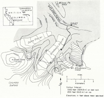
Fig. 1. Map of Athabasca Glacier and vicinity modified from the Jasper National Park Map (1:190 080) distributed by the Canadian Government. Outline shows field area and locations of triangulation stations.
The Field Experiment
Setting. The Athabasca Glacier (lat. 52.2°N., long, 117.2°W.) is located south of the main highway between Banff and Jasper in the Canadian Rockies of Alberta. It is one of several valley glaciers originating in the Columbia Icefield lying on the continental divide go km south-east of Jasper. Figure 1 gives a general map of the glacier and the surrounding terrain.
From the edge of the icefield at an elevation of 2 700 m, the glacier descends, in a distance of 2 km, over a series of three gentle ice falls to an elevation of 2 300 m. The terminus lies at an elevation of 1 920 m. The section between the lowest ice fall and the terminus forms a tongue 3.8 km long with a nearly constant width of about 1.1 km. The geometry of this lower section has been described in detail by Reference Keller, Frischknecht and RaaschKeller and Frischknecht (1961), Paterson (unpublished), Reference Paterson and SavagePaterson and Savage (1963), and Reference KanasewichKanasewich (1963). Reference Paterson and SavagePaterson and Savage (1963) gave extensive information about the pattern of surface motion. Bore-hole measurements by Reference Savage and PatersonSavage and Paterson (1963) gave in addition the variation of velocity with depth at several locations on the glacier. These studies showed a section of the glacier centered 0.8 km below the lowest ice fall to have a particularly simple geometry and surface deformation field. This section, corresponding approximately with the C-section of Reference Paterson and SavagePaterson and Savage (1963), was chosen as being best suited for this field experiment.

Fig. 2. Topographic map of the field area. Bedrock stations are numbered after Reference ReidReid (1961). Topography and elevations are given as shown on the topographical map (1:4 800) compiled in 1962 by the Canadian Government (Topographical Survey, Department of Mines and Technical Surveys, and the Water Resources Branch, Department of Northern Affairs and National Resources) from aerial photography and field survey carried out on 31 July 1962. Elevation of the ice surface on 8 September 1966 was about 10 ft (3 m) lower than as shown. Surface slope measured from the map and computed from 1966 survey data are in agreement.
Field measurements and the local glacier geometry. In the summer of 1966 an array of 9 bore holes and a more extensive grid of surface markers were established. Bore holes and surface markers were arranged in an approximately rectangular grid of longitudinal lines (henceforth referred to as lines and denoted by arabic numerals) and lateral lines (referred to as sections and denoted by capital letters). The arrangement of the lines and the sections and their relationship to features on the glacier surface are shown in Figure 2. The grid spacing was 150 m or approximately half of the center-line depth, except near the margins where longitudinal lines were spaced 100 m apart. The bore holes were in three sections A, B, and C of 5, 3, and 1 holes respectively. Each hole was named according- to its location in the grid (Fig. 2).
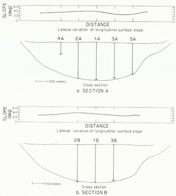
Fig. 3. Cross-section geometry. Cross-section shown is the C section of Reference Paterson and SavagePaterson and Savage (1963). Surface slopes were measured from the 1962 topographic map. Vertical lines represent bore holes of the present study.
Figure 3 shows to what extent the bore holes covered the glacier cross-section as determined by Reference Paterson and SavagePaterson and Savage (1963). It was assumed that all of the holes, except 4A, penetrated to bedrock, although it is possible that some of them were stopped by debris imbedded in the ice slightly above the base. Hole 4A could not be continued below approximately one third of the ice depth because of debris in the ice. In a number of attempts to place bore holes in the marginal zones of debris-covered ice, penetration below depths of about 20 m proved to be impractical for the same reason.

Fig. 4. Center-line geometry and surface strain-rate. Data are from Paterson (unpublished). Heavy line segments in longitudinal profile represent reflecting surfaces observed in a seismic survey. Errors in bed slope are as given by Paterson. Arrows C, A, and B give locations of cross-sections in which bore holes were placed during this field experiment.
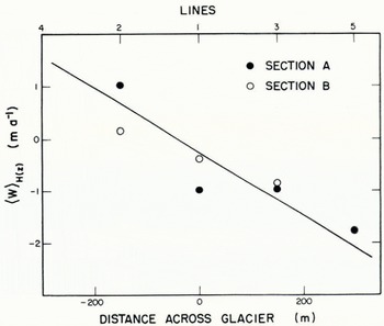
The lateral variation of the longitudinal component of surface slope at sections A and B is shown in Figure 3. The locations of sections A, B, and C in a longitudinal profile along the center-line of the glacier and their relationship to surface and bed topography and to the distribution of surface longitudinal strain-rate are shown in Figure 4. Section A is centered in a region of nearly constant surface slope and uniform longitudinal strain-rate (±10% over a length of two glacier depths).
Motion in the area of the surface marker grid and in the volume of the bore-hole array was measured by determining the initial configuration of the surface markers and bore holes in the summer of 1966 and the deformed configuration about one year later in the summer of 1967. There was essentially complete recovery and measurement of the surface markers and bore holes in 1967. Only the bottom one third of hole 1C was not recovered and measured, A history of bore-hole operations in the summers of ro,66 and 1967 is given in Table I. In 1968 the tops of all bore holes except hole 1C were located, but only two holes (holes 2A and 3B) could be recovered and measured at depth. In this paper only the measurements made between the summers of 1966 and 1967 are discussed.
TABLE I. Chronolooy of bore-hole operations

Field methods. The methods used for making surface and bore-hole measurements were for the most part similar to those which have been used in earlier bore-hole experiments.
The absolute locations of selected surface markers and the surface intersection of bore holes were determined by triangulation. Sitings were made from bedrock stations in a network established by the Water Resources Branch of the Department of Northern Affairs and National Resources (Reference ReidReid, 1961) with a Wild T2 theodolite. Relative locations of all surface markers were determined by tape measurements of the legs and diagonals of the grid rectangles.
The method of boring and recovering holes developed by Reference Kamb and ShreveKamb and Shreve (1966) on the Blue Glacier, Washington, was used on the Athabasca Glacier. In this method holes are bored with electrically powered thermal drills called hot points designed by Shreve (Reference Shreve and SharpShreve and Sharp, 1970). Electricity is supplied by gasoline-powered generators. For electrical and mechanical linkage between a hot point and the glacier surface a sheathed multiconductor cable is used. Bore holes are not cased with pipe; instead a stranded stainless-steel aircraft cable, weighted at the bottom, is lowered down the hole. At a later time, recovery is accomplished by use of a special thermal drill ("cable-following hot point"), which is threaded onto the aircraft cable. Hot points for initial boring of holes are cylindrically symmetric and penetrate the ice vertically. Both types of hot points produce holes about 0.07 m in diameter. Average penetration rates were about 6 m h-1.
During the recovery of the Athabasca Glacier bore holes, periods of extremely rapid hot point penetration (up to six times the normal rate) were experienced at all depths. This indicates that the holes had not closed completely and that the aircraft cable had not migrated normal to itself through the ice. Thus in this case the displacement of cables correctly represented ice displacements. Furthermore it is unlikely that the presence of the cable and the bore hole modified the motion of the ice to any significant degree.
Tilts were measured in initial and deformed bore holes for the purpose of determining their shapes and coordinates at depth. The originally drilled holes were checked for verticality by making tilt determinations every 15 to 20 m. The instrument used for these measurements is a single-shot optical inclinometer loaned by the Parsons Survey Company, South Gate, California. It is a proven instrument identical in mechanism to the inclinometers used previously on several glaciers (e.g. Reference Savage and PatersonSavage and Paterson, 1963; Reference Shreve and SharpShreve and Sharp, 1970). The tilt survey of deformed bore holes was done with a newly developed inclinometer which can be read remotely from the surface (Reference RaymondRaymond, 1971[b]). An electrical output gives the instrument orientation to within 0.1° in tilt magnitude (deviation from vertical) and 20° in azimuth of tilt (direction of tilting) as it was used in 1967. (Subsequently the instrument has been modified to improve the accuracy of azimuth determination.) Its efficiency of operation permitted a much greater density of data to be taken than would have been possible with earlier methods. Measurements were taken at 2 m intervals along the length of the hole, except for the lower 10 to 15 m where a 1 m interval was used.
The possible sources of experimental error associated with the bore-hole measurements in addition to inclinometer instrumental error are: non-parallelism of inclinometer and bore hole made possible by a difference in hole and instrument diameter, wandering of hotpoint on initial emplacement of the hole, non-centering of the aircraft marking cable in the initial hole, fluctuations in the diameter of the hole resulting from changes in hot-point efficiency, spiralling of the cable following hot point around the aircraft cable during bore-hole recovery, and modification of the sides of the hole during the time between boring and the inclinometry survey as a result of flow and freezing processes caused by the presence of the hole.
Coordinates and Notation
Two orthogonal right-handed coordinate systems are used in this paper for the description and analysis of the measurements. In one system (X, Y, Z) the Y axis is directed vertically downward; it is parallel to the initially emplaced bore holes. The X axis has direction parallel to the azimuth of the average surface velocity (N.36.9°.). The origin is left unspecified and is chosen for convenience in the specific application.
In the other system (x, y, z) the z axis is parallel to the Z axis The x axis instead of being horizontal as is the X axis, is taken parallel to the ice surface at the center of the bore-hole array, which has a slope of 3.9°. The surface intersection of hole 1A on 8 September 1966 is taken as the origin of this system (See Figure 2).
The following quantities can be defined with respect to the above coordinate systems. For a fixed choice of the origin of the (X, Y, Z) system, Y8(X, Z, t) represents the elevation of the ice surface at time t. The X and Z components of the surface slope are αX (X, Z, t) = ∂Ys/ ∂X and αZ(X, Z, t) = ∂Ys/ ∂Z respectively. Similarly Yb(X, Z) represents the elevation of the bed, and the X and Z components of the bed slope are βX(X, Z) = ∂Yb/∂X and βZ(X, Z) = ∂Yb/∂Z Let the trace of a bore hole be parametrically represented by Xhb(Y, t) and Zh(Y, t); the X and Z components of tilt of the bore hole are γX(Y, t) = ∂Xh(Y, t) and γz(Y, t) = ∂Xh(Y, t)/ ∂Y. In terms of angular measure, components of tilt are ΓX = tan-1 γz and Γz = tan-1 γz. Similarly these quantities can be defined with respect to the (x, y, z) coordinates and are notated in similar fashion with x, y and z replacing X, Y and Z. The x, y and z components of velocity are denoted by u, v, and w. Tensor components of strain-rate and rotation rate are defined in the usual manner in terms of the gradients of velocity.
With these definitions some of the terms used in the earlier discussion and also in that which follows can be given more precise meaning. Longitudinal surface slope (the longitudinal component of surface slope) is γZ or its equivalent in angular measure. The lateral surface slope is γz = γz or their equivalents in angular measure. Longitudinal and lateral components of tilt are γX (or ΓX ) and z (or ΓZ). Longitudinal velocity is u, and ∂u/∂x represents the longitudinal strain-rate. Transverse motion is represented by the y and z components of velocity v and w; w is referred to as the lateral component of velocity.
Results of Measurements
Surface velocity and strain-rate. Average velocity of stakes measured between September 1966 and July 1967 ranges from 31 m a-1 to 54 m a-1 over the area where theodolite measurements were made. The azimuths of displacement vectors average 036.9°. and deviate from this direction by less than 2º.
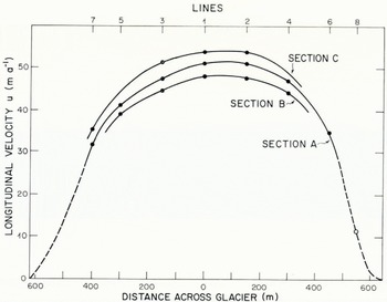
Fig. 5. Lateral variation of surface velocity. Solid circles give velocity of markers determined directly by triangulation. The often circle gives velocity as estimated from measured velocities at adjacent stakes and tape measure.
Lateral variation of average longitudinal velocity u of stakes in sections A, B, and C is shown in Figure 5. The center-line of flow, as defined by the maximum velocity in a lateral profile, falls half-way between line 1 and 2. In section A the profile can be extended essentially to the north-west margin on the basis of tape measurements. These indicate that the longitudinal velocity of stake 8A is 11 m a-1. Extrapolation of the velocity profile indicates that near the margin a zone of decreased velocity gradient must exist, if there is not to be negative (up-glacier) velocity at the margin. On both sides of the glacier the marginal sliding velocity can be no greater than a few meters per year.
The y component of velocity v ranges from — 2.6 m a-1 to 5.6 m a-1. The velocity normal to the surface averaged for all surface markers is 3.5 m a-1. This closely balances the negative annual balance of approximately 3.7 m of ice measured at the surface stakes. Magnitude of lateral velocity at the surface is less than 0.6 m a-1 at all triangulated markers except for 7c and 2c where lateral velocities of 1.22 and —1.30 m a-1 were measured. Values v and w measured at the surface are reported below in conjunction with the values measured at depth. Estimated standard errors for measured velocity of the stakes are 0.20 m a-1 for u and w, and 0.35 m a-1 for v, except at 2B where v may be in error by as much as 0.8 m a-1.
The geometry of the complete surface strain net was determined by tape measurements in early September 1966 and late July 1967. Average surface strain-rate in each grid square was computed by the method of Reference NyeNye (1959[b]). For some squares and rectangles in the out-lying parts of the surface strain net, for which only one diagonal had been taped, a determinate procedure based on the analysis of triangles was used. Over the area of the strain net minimum principal strain-rales range from —0.123 a-1 to —0.015 a-1; maximum principal strain-rates range from —0.002 a-1 to 0.166 a-1.
The distribution of surface strain-rate shows features expected in the ablation zone of a valley glacier. The longitudinal strain-rate is compressive. Within the area of the borehole array éxx ranges from —0.023 to —0.016 a-1; closer to the margins, exx becomes less compressive. The lateral variation of longitudinal strain-rate between sections A and B and between sections C and A can be seen in Figure 5. The lateral extension rate èzz is close to zero over the area of the bore-hole array (-0.002 to 0.005 a-1) but attains greater magnitude locally near the margins. Shear strain-rate èxz has a roughly anti-symmetric distribution about the center-line of flow. Magnitude of èxz within the net attains maximum values of 0.10 to 0.15 a-1 near the north-west margin of the glacier. Standard errors for the measured components of surface strain-rate are 0.001 a-1 or less for all squares and rectangles in the surface strain net.
A complete compilation of the initial locations of all bore holes and surface markers, measured strain-rate, and velocity determinations can be obtained from Raymond (unpublished). In so far as comparison can be made, measured surface strain-rate is compatible with that reported by Paterson (unpublished) for this part of the glacier. The surface velocity measured by Paterson between September 1959 and July 1960 was 15% smaller than that measured in the present study over a similar interval between 1966 and 1967.
Tilting in bore holes. Tilt measurements made in the originally bored holes show the deviations from vertical to be small and the azimuth of non-zero deviations to be random. The root-mean-square deviation from vertical of the components of tilt (Γ x and Γ z ) are 0.25°. Thus the initial bore holes were closely vertical, as could be expected from the symmetry of the boring hot points which were used to drill the holes.
An example of tilt data taken in a deformed hole is shown in Figure 6 and 7. Components of tilt Γ X and Γ z are calculated from the measured magnitude and azimuth of tilt; depth Y is calculated from the measured are length along the hole and the components of tilt. The solid curves are smoothing curves, which were chosen to represent the depth profile of tilting. Smoothing curves were chosen to represent each set of tilt data. For complete compilation of bore-hole tilt data see Raymond (unpublished.
For the most part smoothing curves were chosen by hand drawing best fit curves, as estimated by eye, on plots of the measured magnitudes and azimuths of tilt versus depth. Smooth curves for Γx and Γ z were then calculated from the smoothed distributions of magnitude and azimuth. This procedure has an advantage over the other possibility of directly smoothing the components of tilt, in that certain systematic errors in the azimuth measurement can be reduced. One such systematic effect arises because bearing friction in the compass mechanism of the inclinometer is the main source of instrumental error in determination of azimuth. A slight asymmetry in this error is caused by a tendency of the inclinometer to rotate preferentially in one sense as it is lowered down the hole. This effect can be largely eliminated by taking the center of the well-defined band into which azimuth readings fall, rather than taking the median or a weighted average. A second systematic effect is that any error in an azimuth determination always has the effect of diminishing the calculated component of tilt in the correct plane. This is a second-order effect, but nevertheless, for a 20° error in azimuth, it amounts to 7%, and is thus a systematic effect which should be minimized by eliminating noise in the azimuth determinations before computing the components of tilt. Where the magnitude of tilt approaches zero and the azimuth becomes undefined the above procedure breaks down. For this reason the near-surface portions of several bore holes were handled by direct smoothing of Γ X and Γ Z .

Fig. 6. Longitudinal component of tilt measured in hole 1A on 29 July 1967.
Root-mean-square deviation of the measured components of tilt from the respective smoothing curves is 0.47 º for the longitudinal component and 0.63 º for the lateral component. The generally greater scatter in the lateral components of tilt is an effect of the relatively large error in the azimuth measurement (±20°). For the most part, the scatter in the data is much greater than could be produced by instrumental error (only 0.1° in tilt magnitude); however, it is entirely compatible with the other possible experimental errors enumerated in the section on field methods. Therefore the scatter is most probably experimental noise; there is no compelling reason to attribute any of the scatter to real features of the flow field. On the other hand the possibility that such features exist and contribute to the scatter cannot be discounted. Whatever the sources of scatter, they are not significant with respect to the broad pattern of flow on the scale of the glacier cross-section dimensions, which is of primary concern in this study.

Fig. 7. Lateral component of till measured in hole 1A on 29 July 1967
Bore-hole coordinate profiles. Integration of γ χ = tan ΓX gives the difference in X coordinates of a point on a bore hole at depth Y and the coordinates of the surface intersection of the hole (Y = 0):

The deformed bore-hole coordinate profiles calculated from the smoothed tilt profiles are shown in Figures 8 and 9. For easy comparison they have been normalized to unit time by plotting ΔX(Y, Δt)/Δt and ΔZ(Y, Δt)/Δt, where Δt is the time interval between emplacement of the initially vertical hole and inclinometry after later recovery. All measurement intervals were close to one year (Table I). Bore holes lying on the same longitudinal line are plotted against the same origin. The initial bore-hole configurations are represented by the Y axes.
The deformed bore-hole profiles as plotted represent the differentia] displacement with respect to the surface as a result of ice deformation over the period of one year.
Accuracy of ΔX and ΔZ calculated from Equations (1) can be estimated from the formula
where ΔY is the spacing of lilt measurements, k is the number of intervals ΔY between the surface and depth Y, σγ is the standard deviation of (he component of tilt γX or γZ, and σΔ is the standard deviation of γX or γZ. Equation (2) is valid if the sources of noise are identical at all depths and the individual tilt measurements are independent. If the first of these conditions is assumed to be true, then statistical analysis shows that any dependence between lilt measurements is too weak to be of significance in calculating standard errors for ΔX and ΔZ. At a depth of 300 m, Equation (2) gives standard error of 0.30 m for ΔX and ΔZ in the initially bored holes and respective standard errors of 0.20 m and 0.27 m for ΔX and ΔZ in deformed holes measured after one year. By combining these quantities for initial and deformed holes standard errors of 0,36 m a-1 and 0.41 m a-1 can be assigned to the annual differential displacement in longitudinal and lateral directions at depth 300 m.
Some of the features to be discussed in greater detail below are already apparent from examination of Figures 8 and 9. Measured annual differential displacement between the surface and bed ranges from 5.7 to 13.7 m in the longitudinal direction (Fig. 8), This is much less than the longitudinal velocity of 31 to 54 m a-1 measured at the surface (Fig. 5) and shows that over an extensive area motion is largely accomplished by sliding over the bed or by extremely concentrated shearing in the unmeasured few meters of ice between the deepest tilt measurements and the bed. This is in agreement with observations of Reference Savage and PatersonSavage and Paterson (1963) in a single bore hole (hole 322) which was in the vicinity of the bore holes of this study. Comparison of the profiles of ΔX for bore holes on the same longitudinal line (Fig. 8) shows that the longitudinal strain-rate is progressively more tensile with increasing depth. This agrees with the conclusion reached by Reference Savage and PatersonSavage and Paterson (1963) concerning the depth dependence of the longitudinal strain-rate in this reach of the glacier. Figure 9 indicates the presence of significant lateral flow toward the margins in a roughly symmetric pattern.
Velocity and strain-rate at depth. When the deformation field is simple shear parallel to the y = 0 plane (which approximates the glacier surface), then ![]()
The basic assumption of the method is that the x and z gradients of velocity can be evaluated by comparison of velocity in neighboring holes. This is accomplished by choosing interpolating functions to represent the distribution of the components of velocity on the xz plane at a given depthy. These are differentiated to get x and z gradients. It is further assumed that the ice is incompressible, so


Fig. 8. Longitudinal displacement with respect to the surface as measured in bore holes.

Fig. 9. Lateral displacement with respect to the surface as measured in bore holes.
The distribution of v at a given bore hole must be estimated indirectly. First, it is required to be consistent with the value of v measured at the surface. Second, it is required to be consistent with a zero velocity normal to the bed. This second requirement gives
where the b subscripts on velocity components indicate their values at the bed. At all bore holes, except holes 4A and 5A, both components of bed slope are known from the seismic measurements reported by Reference Paterson and SavagePaterson and Savage (1963) and the differences between depths of holes reaching bed rock. At holes 4Λ and 5A only the lateral component of bed slope is known; at these holes longitudinal slope of the bed is assumed to be equal to that at the surface. The distribution of v between the constrained points at the surface and the bed is calculated from a relaxed form of Equation (3). The method, the basic formulae, and its application to the present measurements are discussed in detail by Reference RaymondRaymond (1971[a]). Some of the results of the analysis are shown in Figures 10, 11, and 12.

Fig. 10. Distribution of longitudinal velocity in valley-glacier cross-sections: (a) measured in section A, (b) measured in section B, (c) computed by Reference NyeNye (1965) for a parabolic channel of width ratio 2. Nye’s solution has been scaled to cover approximately the same range of velocity as observed. Units are m a-1.

Fig. 11. Distribution of longitudinal strain-rate mid-way between sections A and B. Units are a-1.

Fig. 12. Distribution of transverse velocity in (a) section A and (b) section B.
In Figures 10, 11, and 12 the bed and surface geometry in the plotted sections are based on the C section of Reference Paterson and SavagePaterson and Savage (1963), slightly modified to agree with the depths of the holes believed to have reached bedrock (Fig. 3). In these diagrams the flow quantities represent velocity and strain-rate on planar transverse sections parallel to the y axis and the original slake lines across the glacier (Fig. 2). The areal distribution of velocity and longitudinal strain-rate shown in Figures 10, 11, and 12 are based on interpolation between the holes. In section A. where bore-hole data at depth are most extensive, it is possible to estimate the distribution of u outside of the bore-hole array from u measured near the margins at the surface and marginward extrapolation of u determined at depth in the holes (Fig. 10a).
Standard error estimated for u and to is 0.22 m a-1 at the surface and 0.46 m a-1 at 300 m. Error increases approximately as the square-root of depth. Standard error estimated for v is 0.35 m a-1 at the surface and about 0.5 m a-1 at the bed. Standard error for intermediate depth could not be estimated, but it should not greatly exceed 0.5 m a-1. In holes 2B and 5A the error in v can be somewhat larger (0.8 m a-1) because of the possible larger error in the surface value at 2B and uncertainty in the longitudinal bed slope at 5A. For ∂u/∂x a standard error of 0.001 a-1 at the surface and 0.004 a-1 at 300 m depth is indicated. The above estimates apply across the essentially complete width of the sections at the surface and where direct measurement from bore-hole data exists at depth. Velocity for points at depth outside of the bore-hole array is subject to greater uncertainty than quoted above. (For a more complete discussion of errors see Reference RaymondRaymond, 1971 [a].)
Features of the Longitudinal Velocity Field
The main features of the distribution of longitudinal velocity in sections A and B (Fig. 10) are: high sliding velocity over the central portion of die glacier, low sliding velocity al the margins, stronger shear strain-rate near the margins than at the base of the glacier in its central portion, and contours of constant velocity which are approximately semicircular and have shapes significantly different from the cross-section boundary shape.
Sliding velocity. For purposes of discussion, sliding velocity is here defined as the velocity estimated at the bed by extrapolation of the velocity field determined by direct measurement in the bore holes. Beneath seven of the bore holes such extrapolation must be made only over lengths of 2 to 6 m (Table I) or less than 2% of the depth of the glacier. It is possible that the sliding velocily so defined does not represent the existing discrete velocity discontinuity al the ice-rock interface, but rather the combined effects of "true sliding" and an "effective sliding" caused by concentrated deformation in a basal layer beneath the lowermost measurements. For purposes of representing the gross features of the internal velocity field and understanding their relationship to conditions at the surface and bed, the distinction between true and effective sliding is not of direct importance. In terms of large-scale averages the two are not distinguishable. (The distinction is, of course, of great relevance to any discussion of the mechanism of basal sliding.)
One of the most striking features shown in Figure 10 is the high basal sliding velocity, which persists across most of the width of the glacier in both sections A and B. The contribution of basal sliding velocity to surface velocity at the center-line of sections A and B is 81 and 87% respectively. The relative contribution of basal sliding velocity to the surface velocity at a given longitudinal line is only slightly decreased toward the margins. This is supported directly by measurements at hole 5A where basal sliding velocily is still 70% of the surface velocity, and indirectly by the additional constraints placed on the velocity contours outside of the bore-hole array by the surface measurements. A zone of particularly high sliding velocity is centered around line 2 in both sections A and B.
In marked contrast to the sliding velocity of about 40 m a-1 near the center of the channel, the sliding velocity at both margins of the glacier is only a few meters per year. The large lateral gradients in the sliding velocity are particularly significant with respect to any theory of glacier sliding. In addition the great lateral variation in sliding velocity is in strong conflict with the distribution of sliding velocity assumed by Nye in his theoretical analysis of glacier flow in cylindrical channels (Reference NyeNye, 1965).
Shear strain-rate and shear stress at the bed. Shear strain-rate near the bed at the center of the channel contrasts remarkably with that close to the margins (Fig. 10). The values of ∂u/∂y measured at the bottoms of the deep bore holes range from —0.06 a-1 to —0.17 a-1 with an average of -0.10 a-1. In contrast the value of ∂u/∂z at the surface near the north-west margin ranges from 0.2 a-1 to 0.3 a-1. Unless the ice is grossly inhomogeneous in its mechanical properties, the contrast between basal and marginal shear strain-rate implies a similar contrast in shear stress, albeit somewhat weaker because of the non-linear rheology of ice. Thus the glacier is being supported more strongly by "friction" near its margins as compared with “friction” along its base in the center.
A very important consequence of this condition is that the standard procedure for estimating shear stress at the bed gives incorrect results. In the absence of longitudinal stress gradients, the basal shear stress averaged over the area of the bed is easily calculated:

where P and A are respectively the length of the ice-rock contact and the area in the transverse section (Fig. 13), and p is the average density of the ice. The standard assumptions for calculation of shear stress versus depth at the center-line of a valley glacier are that (1) the shear stress at the bottom is equal to the average shear stress at the bed, and (2) the shear stress is linear with depth. Thus,

Fig. 13. Definition of geometrical quantities in a cross-section. H = H(0) is the maximum depth in the section, A = A(W_) is the total area of the section; P is the total length of the ice rock contact.
Where f = A/PH with H being the center-line depth. The quantity f is often called the “shape factor” and has a value of 0.58 for sections A and B. In the present case failure of the first assumption leads to over-estimation of the basal stress at the center-line in sections A and B. Even if the shear stress happens to have linear depth dependence, Equation (5) is incorrect. A quantitative estimate of the error in Equation (5) can be easily obtained for section A. The nearly semi-circular shape of the velocity contours (Fig. 10) indicates that the actual shear-stress distribution would be reasonably represented thereby a dependence corresponding to Equation (5) with f equal to 0.50. This conclusion follows from Nye (Reference Nye1952, Reference Nye1965). Thus in so far as longitudinal stress gradients can be neglected, the second of the standard assumptions is reasonably correct, but the first leads to over-estimation of shear stress by about 16%. This represents a significant failure of Equation (5) in a relatively simple geometrical situation and illustrates a possible source of error in the analysis of all previous bore-hole experiments. A more detailed analysis of the present measurements to give the distribution of stress within the glacier and rheological parameters of the flowing glacier ice will be given in a separate paper.
Flux through the cross-section. A parameter of hydrological interest is the ratio of the average value of a over the area of a cross-section to the average value of u over the width at the surface, that is 〈u〉 A/〈u〉 W. Ice flux through a cross-section is usually calculated under the assumption that this ratio is one. For section A calculation of 〈u〉 A and 〈u〉 W from Figure 10 gives 41.0 m a-1 and 36.5 m a-1 respectively. The ratio 〈u〉 A/〈u〉 W is 1.12. This is significantly different from the value of 1, which is usually assumed. For section A calculation of the average of over depth at the center-line, 〈u〉 H gives 49.6 m a-1. The ratio 〈u〉 A/〈u〉 H is 0.83. Thus, 〈u〉 H gives a worse estimate of 〈u〉 A than 〈u〉 W. The geometrical average of 〈u〉 H and 〈u〉 W, 〈u〉 G = (〈u〉 H/〈u〉 W)½ has a value of 42.6 m a-1 and is a much better approximation to 〈u〉 A than either 〈u〉 W or 〈u〉 H considered singly. This indicates that the distribution of surface velocity is not sufficient for dependable calculation of ice discharge, but that a single bore-hole at the center-line in conjunction with surface measurements can give a considerably more reliable result.
Total ice flux through section A is computed to be 1.09 × 10⁷ m3 a-1.
Comparison with solutions of Nye. Reference NyeNye (1965) computed numerical solutions to the problem of steady rectilinear flow of an isotropic material obeying a power law (n = 3) in cylindrical channels of various cross-sections. He considered only symmetric cross-sections, with sliding velocity everywhere zero, although these conditions are not essential to his numerical method. In particular, a solution for zero sliding velocity is easily converted to one for arbitrary constant sliding velocity by addition of a constant to the velocity solution and leaving the stress solution unchanged. The fundamental assumptions on which the numerical treatment is based are that of rectilinear flow (in which u = u(y, z) and v = w = 0) and homogeneity of the rheological properties. Nye’s solution for a parabolic channel of width ratio 2 is shown in Figure toe. Such a channel geometry approximates quite well the actual sections A and B of the Athabasca glacier, except for the bedrock shelf which may exist on the south-cast valley wall (Reference Paterson and SavagePaterson and Savage, 1963). Figure 10c is identical to Nye’s representation (p. 680, fig. 8a) except that the contours have been relabeled to correspond to a constant sliding velocity of 38 m a-1 and to a scaling appropriate to the observed range of velocities.
Nye’s solution shows certain features which are in agreement with the observed velocity-field. For example Nye predicts that there should be a zone of decreased velocity gradient (∂u/∂z) near the margin as is observed (Figs. 5 and 10a). In addition, his analysis (p. 679) predicts that ∂тxy = —pgx/2 at the surface on the center-line. This accords with the observations,
However, differences between Nye’s solution and the observed pattern oi’ longitudinal velocity are very apparent. This is not surprising in view of the drastic difference between the boundary condition assumed by Nye and the actual distribution of sliding velocity. The most obvious incompatibility between the theoretical and observed distributions is that the relative strength of shear at the margins arid at the base in the center is opposite for the two distributions. As a consequence, the shape factor of 0.646, which corresponds to the linear depth distribution of shear stress т xy, that approximates the theoretical depth distribution at the cenler-line (Reference NyeNye, 1965, p. 679, table IV), is larger than the shape factor of 0.50 which is appropriate to the observed velocity field. A difference in the quantity 〈u〉 A/〈u〉 W also exists. For the parabolic channel of width ratio 2 Nye’s result (p. 677, table III B) is 0.98 when there is no sliding. The value adjusted for the non-zero sliding velocity as represented in Figure to is 0.996. Either of these is distinctly smaller than the observed value of 1.12. These gross differences could probably be rectified by applying a more realistic velocity boundary condition in the theoretical treatment.
By considering the solution to the flow problem for boundaries having the shape of the observed velocity contours, the problem becomes exactly that considered by Nye in terms of geometry and boundary conditions. In this way it is possible to discover whether there are any observable effects arising from the non-rectilinear nature of the flow in the observed sections or from failure of Nye’s rheological assumptions. By considering the width ratios of observed contours it is possible to draw some conclusions without carrying out an explicit solution. The width ratio R is half the distance between the surface intersection of a contour divided by the maximum depth of that contour. Width ratios computed for velocity contours in sections A and B are given in Table II. Nye enumerated some principles based on symmetry which relate the solution in a channel of width ratio R to the solution in a channel of width ratio R-*. These are particularly simple for a boundary with R = 1, which has symmetry such that there is nothing which distinguishes the planes z = 0 and y = 0. This is the case when the boundary has reflection symmetry about the lines at ±45° from the y axis. In this event all velocity contours interior to the boundary must have width ratios equal to one. Consider section A, where the velocity contours are nearly symmetric. Since the contour for u = 46 m a-1 has width ratio one, all contours interior to it should have the same ratio one. This is not the case (Table II), which shows that the longitudinal flow is influenced observably by either the non-rectilinear nature of the velocity field (Figs. 11 and 12) or by inhomogeneity in the rheological properties of the ice.
TABLE II. Width ratio of longitudinal velocity contours

Possible causes of sliding velocity behavior. Since the greatest disparities between theoretical predictions and the observations reported here are probably caused by the large systemmatic lateral gradients in the velocity of sliding, it is important to consider the cause of the observed sliding distribution and whether it is typical of valley glaciers.
For a relation between shear stress and sliding velocity describing stable sliding, shear stress must be an increasing function of sliding velocity when all other parameters are constant. The observations in sections A and B show that there is a relatively lower sliding velocity near the margins where the shear stress is relatively greater. Thus, the observed lateral variation of sliding velocity must be caused by lateral variation of the parameters which affect the relation between stress and sliding velocity, rather than the internal distribution of stress which would exist if such parameters exhibited no lateral variation.
Up to now two parameters have been identified as being important in determining the sliding response to an applied stress. The first is the small-scale topography or roughness of the bed. Although no theoretical analysis of the quantitative effect of bed topography on velocity of sliding has been proven, it seems certain that high bed roughness impedes sliding (Reference WeertmanWeertman, 1964). The second parameter is related to the state of the water between the ice and rock. A correlation between water discharge in streams below glacier termini and variations in surface velocity has been observed on several glaciers (e.g. [Union Géodésiquc et Géophysique Internationale], 1963, p. 65-66; Reference PatersonPaterson, 1964). These observations support the hypothesis that water can have a strong influence on sliding, and indicate that when there is an abundant supply of water, glacier sliding is enhanced. However, the actual mechanism by which water affects glacier sliding is poorly understood and is in dispute. Here it is assumed, as docs Reference LliboutryLliboutry (1968), that the pertinent parameter is the difference between the average normal stress at the ice interface and the water pressure in passageways having access to the bed. When the glacier is sliding stably, it is reasonable to expect that a low pressure difference, corresponding to high water pressure, enhances glacier sliding.
A possible explanation of the observed sliding behavior can be based on the lateral variation of water pressure at the bed. In order to consider this hypothesis in a simple way, it is assumed that the glacier surface is laterally horizontal, that the average normal stress at the ice interface is equal to the ice overburden pressure, and that the pressure in the water at the bed corresponds to a laterally horizontal, hydrostatic water table. The pertinent pressure difference can then be represented as
where z representa the location in the section, H(z) the ice depth there, and δ is the depth of the water level measured below the surface (Fig. 13). The density of water and the density of ice are represented by ρw and ρ respectively. Starting from the deepest part of the section depth H, z = 0) Δρ increases toward the margins and reaches a maximum at a point zδ
where the ice-rock contact intersects the water table. Beyond that point it decreases to zero at the glacier margin. The pressure difference can be considerably larger at zδ
than at the center-line when the water level is high (i.e. as δ approaches 0.1H). This is substantiated by examination of the ratio ![]() as illustrated in Figure 14. With high water levels in a typical valley glacier cross-section, the region of maximum Δρ would be close to the margin, and its retarding effect would tend to produce a smaller marginal sliding velocity than that occurring at the center-line. The effect thus produced would be approximately the same on both sides of the glacier, and would tend to show the largest gradients in the sliding velocity, where the valley sides are steep.
as illustrated in Figure 14. With high water levels in a typical valley glacier cross-section, the region of maximum Δρ would be close to the margin, and its retarding effect would tend to produce a smaller marginal sliding velocity than that occurring at the center-line. The effect thus produced would be approximately the same on both sides of the glacier, and would tend to show the largest gradients in the sliding velocity, where the valley sides are steep.

Fig. 14. Pressure difference and water level. r(δ) gives the ratio of the difference in hydrostatic over-burden and water pressure at the top of the water column (depth δ) to the same difference at the deepest part of the channel (depth H).
If the above mechanism is to provide an explanation for the main features of the distribution of sliding velocity, sliding displacement must occur in the presence of high water levels. Water level was monitored in one of the deep bore holes (hole 2A) for several days in the summer of 1968. The water level fluctuated around an average level of about 40 m below the surface, which corresponds to a value of δ equal to 13H. This observation demonstrates that high water pressure can exist in hydraulic systems deep within the glacier and gives indication that high water pressure at the glacier bed is not unreasonable. Measurements by Reference MathewsMathews (1964) of water pressure in a mine tunnel reaching the base of South Leduc Glacier also give support to this idea.
It is also conceivable that smaller sliding velocity at the margins in comparison with the center-line of a valley glacier could arise from a lateral variation in bed roughness caused by a systematic difference in the glacial abrasion process at the valley sides and on the bottom of the channel. In addition, if the sliding velocity as defined here is not a simple velocity discontinuity at a clear-cut contact between solid bedrock and homogeneous ice, but rather a more complicated phenomenon involving concentrated shearing in a structurally distinct layer of basal ice, there may be pertinent parameters which have not been identified by-existing analyses of basal sliding.
Several features of the distribution of sliding are incompatible with the simplest explanation based on water-pressure variation. The gradient in sliding velocity between lines 3 and 5 (Fig. 10) is much greater than could be expected there on this basis, since the lateral slope of the bed is small. At a corresponding location on the other side of the section there is a maximum in the sliding velocity and a low lateral gradient. These features indicate that either the actual pressure distribution in subglacial water deviates from the assumed distribution or that variations in other parameters must also contribute to the distribution of sliding velocity.
If the observed contrast between sliding near the margins and at the center in sections A and B is indeed caused by the water-pressure effect described above or some fundamental differences in roughness or other parameters on the channel sides and bottom, then it could be a general feature of flow in temperate valley glaciers. It was suggested to the author by Professor W. B. Kamb that some evidence for this comes from surface measurements on several glaciers and their comparison with results of previous bore-hole measurements. Previous bore-hole experiments indicate that although basal sliding is highly variable, on the average it accounts for about 50% of the motion at the surface (Reference KambKamb, 1964). However, sliding velocity at the margins of glaciers is generally considerably less than 50% of the center-line surface velocity. Specific examples are given by Reference MeierMeier (1960, p. 26, fig. 24) for the Castleguard sector of the Saskatchewan Glacier, where marginal velocity is less than 20% of the center-line surface velocity for four transverse profiles spaced roughly 1.4 km apart along the glacier. Other examples are Blue Glacier (personal communication from M. F. Meier), Rhone Glacier (Reference MercantonMercanton, 1916, map no. 3), Athabasca Glacier (Paterson, unpublished, table 12 and figs. 8 to 14) and Austerdalsbreen (Reference Glen and LewisGlen and Lewis, 1961). If sliding velocity is usually smaller near the margins than in the center of the channel in valley glaciers, the present observations probably are an extreme example of the general rule. Nevertheless, theoretical analysis of flow in valley glaciers may be in systematic error until such lateral variation in sliding velocity is taken into account.
Distribution of Longitudinal Strain-Rate
All existing theories of glacier flow require the longitudinal strain-rate ∂u/∂x to be either zero or constant over the glacier thickness. Figure 11 shows this requirement is not satisfied in this section of the Athabasca Glacier. The distribution of ∂u/∂x over the area of the section is in fact quite complex.
Figure 15 illustrates the depth dependence of the compression rate at the three lines where direct data are available. In all three cases there is an approximately linear decrease with depth. Compression rate averaged over depth at line 1 is 0.012 a-1. This agrees very well with the value of 0.014 a-1 predicted by Reference Savage and PatersonSavage and Paterson (1963, p. 4534) for this locality, and supports their conclusion based on similarly made predictions at a number of locations that there are few places along the center-line of the Athabasca Glacier at which longitudinal strain-rate is depth independent. Their work and the measurements of Reference Shreve and SharpShreve and Sharp (1970, p. 82) from bore-hole pairs on the Blue Glacier indicate that compression rate can also increase with depth.
Reference NyeNye (1959[a]) has considered the effects of bending on the distribution of longitudinal strain-rate along the surface of a glacier. Approximately uniform bending would occur if there were a down-stream change in longitudinal slope of the bed, accompanied by a similar change in curvature of the flow lines. Such bending would also cause an approximately linear variation of longitudinal strain-rate with depth and could contribute to the distribution reported here.

Fig. 15. Depth dependence of longitudinal strain-rate
At any point on the glacier surface the rotation rate is given by

since to a very good approximation éxy is zero there. (Equation (6) would be exact if the ice were isotropic and the y axis were everywhere perfectly normal to the surface.) Consequently the bending rate at the surface is

If the bending were uniform then ∂u/∂x would be linear with depth and —∂2v/∂x2 would be independent of depth and give the bending rate. With these conditions the difference in dujdx across the thickness H would be

The bending rate κ can be variously estimated from (a) surface values of ∂u/∂y determined from tilting in two bore holes on the same longitudinal line (giving ∂2u/∂x ∂y), (b) surface values of ∂2v/∂x2 estimated by differencing v measured by triangulation at different stakes on a longitudinal line, (c) by the equation

which is valid to a good approximation when the surface is in equilibrium and the longitudinal gradient in net balance is small, and (d) a similar equation applied at the bed

In the latter estimate, the first and second derivatives of the longitudinal slope of the bed at the center-line can be estimated from the seismic measurements of Paterson (unpublished) (see Fig. 4).
In Table III, the difference in ∂u/∂x across the thickness of the glacier predicted by these various estimates of bending rate are compared with the observed values. The predicted effects of bending are in general too small to account completely for the observed difference in ∂u/∂x. At line 1, the effect of bending based on estimates (b) and (d) are compatible with the observations. However, there is considerable uncertainty in each of these estimates, so the agreement does not necessarily substantiate that bending can account completely for the observed variation with depth of ∂u/∂x. It does seem probable that bending makes a significant contribution at line 1. This may also be the case at line 2. There seems to be no evidence that bending contributes at line 3.
TABLE III. Observed difference in longitudinal strain-rate between the surface and the bed Δ(∂u/∂x) is compared with the effect of bending as estimated from (a) bore-hole tilt data, (b) triangulation data, (c) surface curvature gradient, (d) bed curvature gradient. units are a -1

The areal distribution of ∂u/∂x on the cross-section (Fig. 11 ) is not compatible with a uniform bending rate affecting the whole section. Such an interpretation would require that ∂u/∂x be a linear function of y and z, which is not the case. This fact is of general significance since it is easily shown that even if ∂u/∂x is independent of x, it must be a linear function of y and z in order for the strain-rate field to be independent of x. Thus the distribution of ∂u/∂x illustrates the three-dimensional character of the deformation and indicates that longitudinal stress gradients must be taken into account for the determination of stress within the glacier. The rather complex distribution of ∂u/∂x is probably a combined result of a number of factors such as those acting to maintain equilibrium of the glacier surface, the bending effects cited above, and constraints placed on the longitudinal variation of u at the glacier bed by the parameters which determine the slip velocity.
Features of the Transverse Velocity Field
Motion normal to the main longitudinal component of flow exists as illustrated in Figure 12. The magnitudes of the transverse velocities are smaller than the total longitudinal velocity by more than one order of magnitude. However, the transverse velocities are not greatly smaller than the differential longitudinal velocity between the glacier surface and bed; thus in sections A and B, the transverse motion represents a significant feature of the internal flow. The motion occurs in a roughly symmetric pattern of diverging marginward and surface-ward flow, with the surfaceward component (up to 5.6 m a-1) and the lateral component up to 3.1 m a-1) attaining about equal magnitudes. Most of the lateral transport occurs at depth. In hole 1A, which is near the center-line of the channel, there is relatively strong lateral motion which disrupts the symmetry of the overall pattern.
Transverse velocity at the surface and bed. Where there is net accumulation or ablation, there must be a compensating component of velocity normal to the surface of the glacier in order to maintain equilibrium. For Sections A and B, this is the case within the accuracy of the measurements, and the velocity normal to the surface can be interpreted as being in direct response to the negative net balance which exists in this part of the glacier. The somewhat greater magnitude of the transverse velocity vectors on the south-east (right-hand) side of the glacier in comparison with those on the north-west side shown in Figure 12 is caused in part by stronger ablation on the south-east side of the glacier (Paterson, unpublished) and a geometrical effect caused by the smaller surface slope there (Fig. 3).
The apparent non-zero component of transverse velocity normal to the basal perimeter of the sections is caused by deviation from perfect cylindrical geometry of the bed. The bed does not parallel the x axis; longitudinal bed slope with respect to the x axis (αx ) is +2.0º, +1.2º and —1.0° at lines 2, 1, and 3 respectively. Because of the high basal velocity which exists over most of the width of sections A and B (Fig. 10), these small deviations from cylindrical geometry have a strong effect. In a glacier with smaller basal velocities, similar irregularities in bed geometry would result in smaller transverse velocity at the bed and presumably would cause a smaller perturbation of the flow in the overlying ice.
The pattern of transverse velocity which exists at the surface and bed in sections A and B has detailed features which are related to features of bed geometry and mass balance peculiar to these sections. Nevertheless, the general constraints imposed on the internal flow by the boundary velocities observed in these sections are typical of the ablation areas of valley glaciers. Some of the consequences of non-zero net balance at the surface of a valley glacier are discussed and related to the observed internal flow field in the following sections.
Causes of lateral flow. The dependence of transverse velocity on depth at the center-line of a glacier and its relationship to net balance at the surface, to the geometry of the bed, and to the depth distribution of longitudinal strain-rate have been analysed under the assumption of plane strain, where it is assumed that ![]() (e.g. Reference NyeNye, 1957; Reference Savage and PatersonSavage and Paterson, 1963). However, when the ice depth varies laterally, there are obvious considerations based on the incompressibility of ice which require non-zero lateral transport in order to maintain equilibrium. Some of these have been discussed briefly by Reference NielsenNielsen (1955). Here they are discussed in greater detail in order to understand the pattern of transverse flow observed in sections A and B.
(e.g. Reference NyeNye, 1957; Reference Savage and PatersonSavage and Paterson, 1963). However, when the ice depth varies laterally, there are obvious considerations based on the incompressibility of ice which require non-zero lateral transport in order to maintain equilibrium. Some of these have been discussed briefly by Reference NielsenNielsen (1955). Here they are discussed in greater detail in order to understand the pattern of transverse flow observed in sections A and B.
Consider the average of w over the depth of the glacier H(z) at a given location z in a transverse section x, i.e.

In the ablation zone of a glacier, the ice can be assumed to be incompressible, so that

where A’ is any sub area of the cross-section with boundary C’, and n’ is the outward-pointing normal to C’. Using the notation shown in Figure 13, Equation (9) can be applied to the area A(z) to give

where C̋ is the open curve, with normal n̋, composed of the surface segment and the basal segment of the boundary to A(z).
To consider some of the consequences of Equation (10) in a simple yet generally significant way, it is assumed that the glacier has a planar upper surface (y = 0) and a cylindrical channel with generators parallel to the x axis. Further it is assumed that vs , the value of v at the surface, is uniform across the glacier and ∂u/∂x is constant over the area of the section. Under these assumptions Equation (9) applied to the complete section requires

Equation (10) becomes

For the special case of a parabolic channel
Equation (11) gives

In this case the depth-averaged lateral velocity is zero at the center of the channel and increases linearly toward the margins. In (he ablation zone vs is negative and the lateral motion is toward the margins. Differentiation of Equation (12) gives

At the center of the channel the lateral slope of the bed is zero, so that

and

In the ablation zone where ∂u/∂x is compressive, lateral extension is to be expected. It is important to note that the strength of the lateral extension does not depend on the width ratio of the cross-section but on its shape. (By proceeding directly from Equation (10) it is possible to derive a more general result:

This depends only on the assumptions of a cylindrical glacier geometry, equality of vs at the center-line to its average over the width of the surface, and equality of ∂u∂x averaged over the center-line depth and averaged over the cross-section area. Again it is the channel shape and not the ratio of width to depth which is the determining factor.) The simple results expressed in Equations (12) and (13) indicate that motion toward the margins can be expected to have about the same magnitude as the upward surface-normal velocity. Furthermore, for typical valley glacier cross-sections lateral extension averaged over depth in the central part of the channel is not insignificant in comparison to the longitudinal compression acting in response to ablation.
Interpretation of observed lateral flux. In qualitative terms, the pattern of marginward flow observed in sections A and B is just what would be expected from the above discussion. If the sections are approximated by a parabolic channel of width ratio 2 and ∂u/∂x in Equation (13) is set equal to 〈∂u/∂x〉A as computed from Figure 11 (—0.012a-1), then Equation (13) gives 〈∂w/∂z〉H(0) equal to 0.004 a-1. This compares very favorably with 0.005 a-1 observed at hole 1A and 0.003 a-1 observed at hole 1B. If vs in Equation (12) is set equal to its average across the surface (3.8 m a-1), then "predicted" lateral transport as a function of distance across the glacier can be calculated from Equation (12). In Figure 16, this is compared with the lateral transport observed at the bore holes. Although there are some discrepancies, there is a clear correspondence between the observed values and the predicted distribution. These comparisons indicate that the general pattern of the observed motion represents the type oftransver.se velocity field which can be expected 10 be typical of valley glaciers in the ablation zone. The discrepancies exist because the assumptions used in the derivation of equations do not apply exactly. Sections A and B are only approximately parabolic (Fig. 13); cylindrical geometry exists only to a first approximation (Figs. 3 and 4): v is not uniform across the surface (Fig. 12); ∂u/∂x is not uniform on the sections (Fig. 11). The resolution and coverage of the bore-hole measurements is not sufficient to make it possible to give dependable explanations of deviations from the predicted flow in terms of specific features of the bed geometry and the distribution of longitudinal strain-rate.

Fig. 16. Comparison of depth-averaged lateral velocity predicted from Equation (12) (solid line), observed in section A (solid circle), and observed in section B (open circle).
Lateral surface elevation differences. A detailed analytical investigation of the transverse flow pattern involving the actual depth distribution of v and w and the specific lateral surface profile needed to produce the requisite driving stresses is a difficult non-linear boundary-value problem. This will not be considered here. It is possible, however, to make a simple order-of-magnitude estimate of the elevation difference between the central and marginal parts of the glacier surface which is necessary to drive the observed lateral flux.
Consider the problem of a rectangular region of depth H and width W, which is occupied by a Newtonian fluid of viscosity η At the top of the slab (y = 0) a sinusoidally varying normal stress is applied
where N is positive and h=2π/W. The shear stress τyz is zero there. On the bottom (y = H) and the lateral margins (z = ±W/2) of the slab, the velocity normal to the boundary and the shear stress parallel to the boundary are zero. The solution to this problem can be derived by standard analysis of the biharmonir equation and is considered in detail by Raymond (unpublished). The maximum lateral flux qz max in the slab occurs at z = ± W/4 or half-way between the center and lateral margins of the slab, and is related to the normal stress amplitude N by

The above problem is different from the one of interest. Most obvious is the difference in bed shape and the shear stress acting there. The boundary condition applied to the planar upper surface of the slab also differs from the natural boundary condition in which the convex upward glacier surface is stress free. The natural condition can be approximated by taking the surface of the slab to have the mean elevation of the true glacier surface, and by taking normal stress on the slab surface to be the weight of the overlying material between the slab surface and the actual glacier surface. In general, this would not have a sinusoidal lateral variation. But it is reasonable to suppose that the magnitude of the lateral transport is determined mainly by the total elevation difference between the center and margins ΔH and is less strongly dependent on the specific shape of the surface; thus
is a reasonable correspondence. The assumed constant viscosity of the slab material is a considerable simplification. In reality, the effective viscosity at depth is less than that near the surface as a result of the large strain-rate associated with the longitudinal flow. However, by taking an appropriate average viscosity a reasonable correspondence between the slab and the glacier should exist. On the basis of the observed strain-rates éxy and standard assumptions about τxy , an average viscosity of about 10 bar year is reasonable.
If now it is assumed that the maximum lateral flux in sections Λ and B can be represented by the flux observed at hole 5A (which is about half-way between the center-line and the south-west margin and shows an average lateral velocity of 1.8 m a-1 over a depth of 260 m), then with W = 1.2 km the required normal stress amplitude is 0.36 bar as given by Equation (14). This corresponds to an elevation difference between the center and margins of 7.8 m. The existing elevation differences are 7.6 m for the south-east side and 6.1 m for the northwest side. In view of the many simplifications made in the above calculation, this exceptionally good agreement must be regarded as being somewhat fortuitous. Nevertheless, it indicates that the existing "central hump" on the Athabasca glacier produces stresses which can reasonably account for the magnitude of the observed lateral transport.
Depth distribution of the lateral flow. Most of the lateral transport in sections A and B occurs at depth (Fig. 12). This is somewhat akin to extrusion flow as envisioned by Reference DemorestDemorest (1943). Although extrusion flow has been discredited as a mechanism for the longitudinal component of flow, it may represent the normal pattern of transverse flow associated with the convex lateral surface profile in the ablation area of valley glaciers. (Correspondingly where there is positive net balance on a valley glacier, transverse intrusion flow may be representative.) The problem of how the upper layers of ice can be equilibrated when they are resting on a stratum of faster moving ice, which was overlooked by Demorest, does not necessarily arise in this case because of the lateral confinement imposed by the valley walls. (The pattern of motion calculated for the rectangular slab considered in the preceding section gives some support to the above hypothesis. Across the full width of the slab, lateral velocity at its base is 2.5 times greater than at its surface.)
If this hypothesis is true, measurement of small lateral velocity w and strain-rate ézz on the surface of a valley glacier in the accumulation or ablation area should not be taken as evidence that they are equally small at all depths.
Acknowledgements
I am particularly grateful to Professor Barclay Kamb for many stimulating discussions which contributed to progress in all phases of this research. The success of the field program is due in large measure to the foundations built up over many years at the California Institute of Technology by the combined efforts of Professors Kamb, Sharp, and Shreve. Dr William Harrison and Messrs Terry Bruns and Don Lashier assisted in the field work.
The Canadian Government gave permission to work in Jasper National Park and allowed the entry of field equipment into Canada. Special thanks go to Bill Ruddy and Chester Kongsrude of Snowmobile Tours, Ltd., who generously provided transport of equipment and supplies on the glacier.
During the period of this research I was supported by a. National Science Foundation Graduate Fellowship. Research expenses were funded by National Science Foundation Grant GP-5447. I am grateful to the University of Washington for support during preparation of the final manuscript and for providing part of publication costs under National Science Foundation Grant GU-2655 and Office of Naval Research Contract N0014-67-A-0103-0007. NR 307-252.
MS. received 19 June 1970 and in revised form 27 September 1970