


Impact Statement
To develop machines for fusion power, obtaining models that scale with the machine size is a paramount issue. A magnetised target fusion (MTF) power plant, for example, exhibits cavity surface disturbances that will vary with the design parameters of the machine. The present results indicate that, for initial disturbances, the dominant scalable parameters are the geometric factors (the initial surface position relative to submerged obstacles) and the initial surface acceleration. Interestingly, fluid properties such as viscosity, surface tension and density do not explicitly appear in the analysis for high Froude numbers  $Fr$ (high inertia to gravity effects ratio). For small $Fr$, we do observe the influence of viscosity and surface tension; the experimental free surface is observed to be smoother than the corresponding analytical results from potential flow models. Therefore, analytical models can be used for designing worst-case scenarios in applications in which it is critical to diminish surface perturbations and jets, such as the design of imploding cavities in MTF plants.
1. Introduction
Generating energy via MTF relies on the rapid compression of magnetised plasma to fusion conditions (Reference Kirkpatrick, Lindemuth and WardKirkpatrick, Lindemuth, & Ward, 1995). General Fusion is developing an MTF concept on which fusion is achieved by first rotating a liquid metal liner inside a rotating core to create a quasi-spherical cavity into which magnetised plasma is injected, as shown in figure 1(a). Pistons are then used to impulsively push the liquid out of a series of radial channels (see zoom-in of figure 1b), which in turn causes the liner to move radially inwards, collapsing the cavity and hence compressing the plasma to fusion conditions (Reference LabergeLaberge, 2019). To maintain plasma stability during compression, it is critical that disturbances on the liner–cavity interface (see zoom-in on the right of figure 1b), which is initially some distance in front of the channel walls, are kept to a minimum i.e. the interface is as smooth as possible (Reference Avital, Suponitsky, Khalzov, Zimmermann and PlantAvital, Suponitsky, Khalzov, Zimmermann, & Plant, 2020; Reference Huneault, Plant and HigginsHuneault, Plant, & Higgins, 2019). Due to the initial proximity of the interface to the walls of the channels, it is reasonable to assume that the onset of any disturbances is due to the interaction of the liquid with these walls, and will depend on the acceleration of the liquid, the initial distance of the interface from the end of the channels and the geometry of the channels. To explore the origins of such disturbances, we idealise the problem to that of a liquid being impulsively accelerated past a single cylindrical obstacle over a finite time interval, as represented with a yellow circle in panel (c) of figure 1. As such, the cylindrical obstacle represents the wall between two consecutive channels, whilst the finite time interval confines the problem to the initial motion of the interface, where the interface has moved a distance comparable to that of the wall (cylinder) thickness. Finally, the rapid acceleration of the fluid allows one to consider potential flow solutions to such problems which, if verified experimentally, can then be readily expanded to the multiple obstacle configurations, such as those seen in the actual machine (figure 1b).

Figure 1. (a) Artistic rendering of the lateral view of a MTF power plant. (b) Zoomed-in view of the initially disturbed surface as pusher pistons move the liquid metal through radial channels. (c) Zoomed-in view of (b), where a single channel wall is represented as an equivalent circular obstacle that disturbs the moving free surface of the liquid metal liner.
Prior studies on the interaction between a moving free surface and submerged obstacles primarily focused on the canonical system of a submerged cylindrical obstacle in a two-dimensional semi-infinite fluid. Reference LambLamb (1913) modelled the circle as a dipole potential, modified to satisfy linearised free-surface conditions, which produced a satisfactory solution to the surface perturbations, but was limited to small disturbances on the free surface. This was later extended by Reference HavelockHavelock (1927, Reference Havelock1936), who constructed a complete solution to the linear problem. Later, Reference Wehausen and LaitoneWehausen and Laitone (1960) designed a recursive scheme for the linearised problem, whilst Reference TuckTuck (1965) extended the approach by Reference Wehausen and LaitoneWehausen and Laitone (1960) to address nonlinearities on the free surface. The works by Reference TelsteTelste (1987), Reference GreenhowGreenhow (1988), Reference Teles da Silva and PeregrineTeles da Silva and Peregrine (1990), Reference TerentevTerentev (1991) and Reference Guerber, Benoit, Grilli and BuvatGuerber, Benoit, Grilli, and Buvat (2012) rely on numerical simulations to analyse the full initial/boundary value problem of the forced motion of a submerged cylinder and its interaction with the free surface. Analytical works to describe the full nonlinear problem, however, are usually limited to the initial development of the perturbation. Reference Tyvand and MilohTyvand and Miloh (1995) used conformal mapping to bipolar coordinates to obtain a Taylor time series expansion of the surface perturbation. Reference MakarenkoMakarenko (2003) and Reference Kostikov and MakarenkoKostikov and Makarenko (2018) explored an alternative method for computing the short-time triggering of nonlinear effects based on the transformation of the full domain equations into a boundary integro-differential system, defined only on the free surface. While analytical expressions were obtained independently by Reference Kostikov and MakarenkoKostikov and Makarenko (2018) and Reference Tyvand and MilohTyvand and Miloh (1995) for surface perturbations up to the fourth order in time, only the method by Reference Kostikov and MakarenkoKostikov and Makarenko (2018) proved to be easily extendable to higher orders, as well as submersion motions different from constant acceleration or constant velocity. Such an investigation was conducted by Reference Martín Pardo and NedićMartín Pardo and Nedić (2021), who analysed the influence of the obstacle size, the initial surface level and the liquid acceleration profile on the resulting surface perturbations. Reference Martín Pardo and NedićMartín Pardo and Nedić (2021) developed a recursive semi-analytical method to obtain higher-order accuracy of the surface perturbation in both time and space. A marginal gain in accuracy, however, was observed as higher-order solutions were implemented. To the best of our knowledge, there is no rigorous experimental validation of the analytical models cited above in the literature.
Reference Tyvand and MilohTyvand and Miloh (1995), Reference Kostikov and MakarenkoKostikov and Makarenko (2018) and Reference Martín Pardo and NedićMartín Pardo and Nedić (2021) provide approximations of different orders to the temporal series for nonlinear surface disturbances, but are limited to a finite prediction time. After such prediction times, the analytical solutions grow unbounded without any resemblance to the physical system itself. How well and for how long these approximations hold needs to be validated experimentally. Moreover, these analytical models are based on potential flow theory, and therefore neglect viscous and surface tension effects; see, for example, the study of Reference Moreira and PeregrineMoreira and Peregrine (2010) who analysed surface tension effects on the free surface and the nonlinear features that emerge as a result, in particular the appearance of capillary–gravity waves. It remains unclear how these effects will change the surface as compared with the results provided by these models. To answer these critical questions, we developed an experimental facility where a liquid is impulsively accelerated around a circular cylinder, and compared the results with the analytical models by Reference Tyvand and MilohTyvand and Miloh (1995), Reference Kostikov and MakarenkoKostikov and Makarenko (2018) and Reference Martín Pardo and NedićMartín Pardo and Nedić (2021).
The second objective is to determine the critical parameters for which surface disturbances result in jetting, the most adverse condition in the application of MTF. Jetting is usually described as a collimated stream of liquid that results from hydrodynamic instability and singularity formation on a liquid surface (Reference Cruz-Mazo and StoneCruz-Mazo & Stone, 2022; Reference EggersEggers, 1993; Reference Lai, Eggers and DeikeLai, Eggers, & Deike, 2018). Although prior studies have classified jetting and gravity waves based on empirical observations (Reference Martín Pardo and NedićMartín Pardo & Nedić, 2021; Reference ReinRein, 1996; Reference Zhao, Brunsvold and MunkejordZhao, Brunsvold, & Munkejord, 2011), we believe an approach which utilises highest standing wave theory (Reference GrantGrant, 1973; Reference OkamuraOkamura, 1998; Reference Penney, Price, Martin, Moyce, Penney, Price and ThornhillPenney et al., 1952; Reference TaylorTaylor, 1953) may provide a physical foundation to the classification of surface disturbances into jetting or gravity waves.
2. Experimental set-up and system parameters
A custom facility, the frontal view of which is shown in figure 2, was developed to measure free-surface disturbances on an accelerating liquid. In each experiment, a double-piston assembly pushed a mass of water past an initially submerged cylindrical obstacle. The system was set into motion via the expansion of compressed gas from a reservoir, released with the opening of a solenoid valve. A thorough description of the different components of the apparatus can be found in § 1 of the supplementary material available at https://doi.org/10.1017/flo.2022.29. The moving free surface was recorded using high-speed imaging. Two sample video frames for one of the experiments are shown in figure 3; figure 3(a) corresponds to an instant before the fluid is set into motion, whilst figure 3(b) shows a later time when disturbances are clearly visible. The circular obstacle boundary is delimited by a blue circle in the figures. A Cartesian coordinate system is fixed with the  $x$-axis along with the initial planar position of the liquid surface and the $y$-axis passing through the centre of the obstacle, directed vertically upwards. The obstacle of radius $R$ is located at the coordinate $x=0$, $y = -H_0$, where $H_0$ is the initial depth of the surface relative to the obstacle. The time $t$ is measured from the initiation of the liquid motion. The instantaneous surface profiles are detected by an edge-tracking algorithm, indicated as red curves in figure 3, from which the surface profile height $\eta (x,t)$ and the average surface height $\bar {\eta }(t)$ can be measured (figure 3b). Since at $t\le 0$ the surface is planar (figure 3a), it follows that $\eta (x,t=0) = \bar {\eta }(t=0) = 0$. For conditions where a rising central column develops in the surface, as shown in the inset of figure 3(b), the width $W(t)$ between the local minima of the column, and the prominence $P(t)$ of the peak, is utilised to analyse the evolution of this central column.

Figure 2. Diagram of the experimental apparatus (not to scale).

Figure 3. Video frames of one experiment with the coordinate system and main geometric variables utilised to describe surface perturbations (a) before ( $t < 0$) and (b) after ( $t > 0$) the beginning of the motion.
The average surface height  $\bar {\eta }(t)$ depends only on the geometric parameters $R$ and $H_0$ and on the initial gas pressure $P_0$ in the reservoir. A total of 260 experiments were conducted for this work, with input parameters in the ranges $2.5\ \mathrm {mm} \le R \le 7.5\ \mathrm {mm}$, $R\le H_0\le 5R$ and $0.2\ \mathrm {MPa} \le P_0 \le 0.7\ \mathrm {MPa}$. The particular selection of these bounds corresponds to an optimal functioning of the experimental device and to the mitigation of wall effects from the water tank. See § 1 of the supporting material for further discussion on these inputs limits.
Figure 4 shows five representative motion curves  $\bar {\eta }(t)$ for different values of $P_0$ for a set-up with $R = 8$ mm and $H_0 = 10$ mm. Each dash-dot line shows the 10-value moving average of measured values, with the bands indicating the standard deviation of the moving windows. Continuous lines indicate constant acceleration parabolas of the form $at^2/2$ that have been fitted to each $\bar {\eta }(t)$ curve. Note that the acceleration of the average surface height $\bar {\eta }(t)$ corresponds to the rate of change of the volumetric flow rate per unit area of the fluid as it moves through the water tank. As a first approximation, and to allow for systematic comparison between experiments and theory, we assume that the acceleration of the interface is approximately constant for times where the parabola fit lies within the uncertainty bounds of the experimental data $\bar {\eta }(t)$. The times at which this assumption is no longer valid are shown as white circles in figure 4. Under this premise, each motion function $\bar {\eta }(t)$ can be parameterised only by the fitted acceleration constant $a$. Similar fits to those shown in figure 4 were obtained for measurements from experiments with other values of $R$,
$R$,  $H_0$ and $P_0$.

Figure 4. Temporal dependence of the average surface height  $\bar {\eta }(t)$ for a set-up with an obstacle radius of $R = 5.0$ mm, an initial surface depth of $H_0 \approx 6.3$ mm and different initial gas pressures $P_0$. Dashed lines represent measured 10-value averages and coloured bands show the corresponding standard deviation. Parabolas (solid lines) correspond to the best fit of a constant acceleration profile departing from rest for each experimental curve. White circles denote the time validity of the constant acceleration assumption.
To characterise the evolution of the surface disturbance with time, we will analyse the perturbation height, defined as  $\Delta \eta (t) \equiv \max _x \eta (x,t) - \min _x \eta (x,t)$. Like the average surface height $\bar {\eta }(t)$, the perturbation height $\Delta \eta (t)$ depends only on $R, H_0$ and $P_0$. In particular, the dependence on $P_0$ can be conveniently substituted by the dependence on $\bar {\eta }(t): \Delta \eta ( t) = f_1 (R, H_0, \bar {\eta }(t); t)$, where a semicolon has been used to separate the parameters $R$,
$R$,  $H_0$ and $\bar {\eta }(t)$ that define the functional form of $f_1$ from the variable $t$. Utilising the motion profile instead of the initial gas pressure detaches our analysis of the particularities of the experimental apparatus, thus making it applicable to general moving surfaces and submerged obstacles. Moreover, if we restrict our study to the time for which the motion of the surface is one of constant acceleration, $\Delta \eta (t)$ can be simplified to $\Delta \eta ( t) = f_2 (R, H_0, a; t)$. In order to facilitate the comparison between our results and those found in the literature, we introduce the characteristic velocity
 \begin{equation} \bar{U} = \sqrt{\frac{a H_0}{2}}, \end{equation}
which corresponds to the average velocity of the surface position  $\bar {\eta }(t)$ between $t= 0$ and the characteristic time $t= T$, defined as the time taken for the surface to move its own initial depth $H_0$, that is $\bar {U} = {H_0}/{T}$, with $T$ defined such that $\bar {\eta }(t=T) = H_0$. The system variables are non-dimensionalised using $H_0$ as a spatial scale and $T$ as a time scale (see, for example, Reference Tyvand and MilohTyvand & Miloh, 1995). Throughout this work, we denote with a starred variable $x^*$ the non-dimensional counterpart of the corresponding dimensional variable $x$. We thus obtain the non-dimensional perturbation amplitude $\Delta \eta ^* \equiv \Delta \eta /H_0$ as a function of only two dimensionless independent groups, and of the non-dimensional position $x^*\equiv x/H_0$ and time $t^*\equiv t/T$: $\Delta \eta ^* ( t^*) = f_3( r^*, \lambda ;t^*)$ where $r^*$ is the obstacle radius to initial depth ratio
 \begin{equation} r^ * = \frac{R}{H_0}, \end{equation}
and  $\lambda$ is the inverse squared Froude number
 \begin{equation} \lambda = (g + a) H_0 / \bar{U}^2. \end{equation}
Here, the apparent gravity  $g+a$ felt in a fixed-obstacle reference frame is used to facilitate a comparison of the experimental results to numerical/analytical studies found in the literature, e.g. Reference TerentevTerentev (1991) and Reference Tyvand and MilohTyvand and Miloh (1995). Combining equations (2.1) and (2.3), we obtain a definition for $\lambda$ under the assumption of constant acceleration
 \begin{equation} \lambda = 2 + g H_0/\bar{U}^2, \end{equation}
which shows that  $\lambda \geq 2$. Although $r^*$ and $\lambda$ have been used in previous studies, we propose to use the variables
 $$\begin{gather} H^ * = \frac{H_0}{R} -1 \equiv \frac{1- r^ * }{r^ * } \quad \mbox{and} \end{gather}$$
 $$\begin{gather}{Fr} = \frac{1}{\sqrt{\lambda}}, \end{gather}$$
which are more relatable to experimental conditions. Therefore, the functional form of  $\Delta \eta ^* ( t^*)$ to be analysed in this work is $\Delta \eta ^* ( t^*) = f( H^*, {Fr}; t^* )$. The non-dimensional fill depth $H^*$ indicates the distance between the initial free surface and the highest point of the cylinder surface, i.e. $H^* = 0$ corresponds to the initial free surface being initially tangent to the cylinder while $H^* = 5$ means it is five radii away from this point. The Froude number $Fr$ is the ratio between inertia and apparent gravity forces at the surface, with larger $Fr$ values indicating faster fluid motions relative to apparent gravity effects.
3. Identification and classification of jetting and gravity waves
3.1 Perturbation features
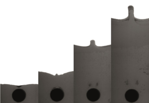
Frame sequences from two representative experiments are shown in figure 5, one (figure 5a) corresponding to conditions that lead to the creation of jetting, the other corresponding to a free surface with gravity waves (figure 5b). For the jetting case, figure 5(a), the obstacle radius was  $R = 5.0$ mm, initial surface depth $H_0 = 6.4$ mm and with a characteristic liquid velocity of $\bar {U} = 0.61$ m s $^{-1}$, whilst for the gravity wave case figure 5(b) the radius was $R = 5.0$ mm, initial surface depth $H_0 = 13.1$ mm and $\bar {U} = 0.57$ m s $^{-1}$. The corresponding recorded videos of these two experiments can be found in the supplementary material to this article. Note that, since the values of $H_0$ and $\bar {U}$ are different for the two experiments, the non-dimensional times $t^*$ of each frame evolve differently for equal dimensional times $t$ in figure 5.

Figure 5. Features that emerge on the free surface for (a) jetting, and (b) gravity wave. The surface shown in (a) corresponds to experimental settings  $R = 5.0$ mm, $H_0 = 6.4$ mm and $\bar {U}= 0.61$ m s $^{-1}$ ( $H^* = 0.28, Fr = 0.70$), while the surface shown in (b) corresponds to $R = 5.0$ mm, $H_0 = 13.1$ mm and $\bar {U} = 0.57 (H^* = 0.38, Fr = 0.64 )$ m s $^{-1}$. Dimensional and non-dimensional times have been annotated on each frame.
At  $t=10$ ms, the initially planar free surface has developed a central depression above the cylinder. The depth of the depression is different for both cases. This is expected, given the different initial surface depths $H_0$. Also, a deeper central depression can be observed for the shallower initial depth. By $t=15$ ms, a central wave starts to appear for both cases. Critically, we note that the central wave for the jetting case is narrower as compared with the gravity wave case. By $t=20$ ms, the central waves grow in amplitude for both cases, but the morphology of the waves is quite different. For the jetting case, a strong, thin jet, with very steep slopes appears, where droplets (in the form of a spray) will detach from the bulk of the fluid, carrying perturbation energy along with them. The gravity wave case, on the other hand, begins to subside and the perturbation energy will be dispersed as a gravity wave. The two cases shown in figure 5 have both different initial fill depths $H_0$ and were driven at different characteristic velocities $\bar {U}$. By altering these two parameters for each experiment, one can obtain free-surface perturbations that vary in morphology as has been discussed here, and that can be categorised as either a gravity wave or a jet.
3.2 Central column steepness
As mentioned in § 1, the presence of jets on the free surface can be detrimental to the MTF application. Therefore, being able to predict the conditions under which each perturbation regime is observed is of practical importance. Except for cases where the surface keeps an almost planar form during its motion (for small fluid velocities  $Fr \lessapprox 0.35$ and/or large initial depths $H^* \gtrapprox 4.0$), a central depression in the moving surface is observed, followed by the formation of an emerging liquid column around $x=0$ (see inset in figure 3b). In this section, we show how the analysis of the evolution of this central liquid column can be utilised to find the limiting set of parameters $H^*$ and $Fr$ that separate a smooth surface, where gravity waves are present, from one where jetting onsets.
It is reasonable to assume that the central liquid column may no longer sustain its shape, and hence break into a jet, when its height becomes too large for its width, i.e. the column becomes too steep. Finding the limiting breaking steepness for the cases of standing waves and progressive waves has been studied extensively in the past (e.g. Reference Penney, Price, Martin, Moyce, Penney, Price and ThornhillPenney et al., 1952; Reference TaylorTaylor, 1953). Notice that, in the moving obstacle reference frame discussed previously, the average surface height is quiescent and the central column can be studied as a solitary standing wave. We shall, therefore, rely on the theory of highest standing waves to obtain a breaking limit for the observed central column.
The study of highest standing waves before reaching the breaking limit was first conducted by Reference Penney, Price, Martin, Moyce, Penney, Price and ThornhillPenney et al. (1952), who postulated that these waves break when the peak angle reaches a value of 90 $^\circ$, corresponding to a maximal slope of 45 $^\circ$ on its surface. Under this condition, the particles at the tip of the wave face a zero pressure gradient, and so fall freely under gravity at the maximum height. The assertion of the 90 $^\circ$ peak angle by Reference Penney, Price, Martin, Moyce, Penney, Price and ThornhillPenney et al. (1952) for the highest wave was later corroborated experimentally by Reference TaylorTaylor (1953) and theoretically by Reference GrantGrant (1973) and Reference OkamuraOkamura (1998).
The well-established topic of highest progressive periodic waves in deep water, which is related to, but is different from, highest standing waves, was pioneered by Reference StokesStokes (1880) using classical nonlinear wave theory. Reference StokesStokes (1880) showed that the highest progressive waves have a peak angle of 120 $^\circ$, which corresponds to a maximum slope of 30 $^\circ$ on the liquid surface. Defining the steepness of a wave as the ratio of its prominence $P$ to its width $W$ (see inset in figure 3), i.e. $s \equiv P/W$, (Reference Schwartz and FentonSchwartz & Fenton, 1982), using numerical computations, produced the currently established value of $s_{br} = 0.1412$ for the maximum attainable steepness for travelling deep water waves before breaking. The maximum slope angle for a standing wave of 45 $^\circ$ is 50 $\%$ greater than the steepest slope angle of $30^\circ$ for a progressive wave. Therefore, the maximum steepness should be approximately 50 % higher for standing waves than for progressive waves, that is $s_{br} \approx 0.2118$. This elementary estimate holds notably well, when compared with the values obtained by Reference GrantGrant (1973), Reference Schwartz and WhitneySchwartz and Whitney (1981), Reference Tsai, Jeng and HsuTsai, Jeng, and Hsu (1994) and Reference Tyvand and NølandTyvand and Nøland (2021). These authors arrive by different methods to maximal values in the range $0.204\leq s_{br}\leq 0.213$. In this work, we will utilise a value of $s_{br}=0.2$, which gives the needed accuracy for determining whether a central column reached its breaking limit in our experiments.
The central wave steepness for a selection of  $Fr$ and $H^*$ is shown in figure 6. For cases where the shape of the wave could no longer be accurately tracked due to the formation of splashes and droplets, the continuous line has been replaced by dashed lines in figure 6. Before the onset of a central column, the steepness is approximately zero, after which the steepness parameter begins to increase as the central column grows. This growth is initiated at later times for larger $H^*$ (around $t^* = 2$ for $H^*=2.33$ in figure 6a) and at earlier times for smaller $H^*$ (around $t^* = 1.0$ for $H^*=0.43$ in figure 6d). Moreover, the rate at which the steepness increases is slower for bigger $H^*$, which is evident by comparing, for example, the slopes of the curves for $H^*=2.33$ with those for $H^*=1.50$, 0.67 and $0.43$. For equal $H^*$ values, the initial growth rate seems to be related to $Fr$. Smaller $Fr$ (smaller characteristic velocities) result in slower column growth; see, for example, the $H^*=2.33$ curves for $Fr$ values of $0.40$ and $0.75$. In certain cases, after the initial growth phase, the steepness begins to decrease, e.g. for $H^*=0.67, Fr = 0.58$, eventually reaching a plateau, whilst for other cases, namely $Fr > 0.51$ and $H^*=0.67$, it continues to grow unbounded, with splashes observed at the tip of the wave. When the latter occurs, and for a given $H^*$, the maximum height of the column is typically lower for smaller $Fr$ values. For example, in figure 6(d), the maximum steepness of the initial plateau is $0.47$ for $Fr = 0.69$, $0.41$ for $Fr = 0.67$ and $0.35$ for $Fr = 0.50$. For the smaller $Fr$ cases, or equivalently slower characteristic velocities, the plateau is not observed within the field of view of the experiment, although one is expected to be seen had the field of view been increased.

Figure 6. Wave steepness evolution for experiments with multiple values of  $H^*$ and $Fr$. The 10-value moving average and the corresponding standard deviation are plotted in the form of continuous lines and transparent shades of the same colour; (a) $H^* = 2.33$, (b) $H^* = 1.50$, (c) $H^* = 0.67$ and (d) $H^* = 0.43$.
In figure 6, the breaking wave threshold of  $s_{br}=0.2$ has been indicated with a dashed grey line. All the experiments shown in figure 6(a) for $H^* = 2.33$ and in figure 6(b) for $H^*=1.50$, $Fr \le 0.65$ cases have steepness curves that remain below the breaking wave limit at all measured times. For the faster fluid motion ( $H^*=1.50$, $Fr = 0.69$) figure 6(b) shows that the wave steepness surpasses the threshold and continues to grow unbounded. A similar behaviour is observed for the case $H^* = 0.67$. However, the surface motion needs to be slower than $Fr = 0.51$ for the column steepness to remain bounded by the limiting threshold. Finally, for $H^*=0.43$, we see that the steepness curves for all velocities consist of an initial rapid growth region (e.g. $Fr = 0.69$ in the range $0< t^*<1$), followed by plateaus, within high uncertainty (e.g. $Fr = 0.69$ in the range $1< t^*<1.7$), and then periods of erratic behaviour (e.g. $Fr = 0.69$ for $t^*>1.7$). The initial growth for these cases corresponds to the formation of a central depression (e.g. figure 5(a) at 10 ms). The plateau indicates that a jet is forming inside the depression (e.g. figure 5(a) at 15 ms). The jet continues to grow until its tip surpasses the uppermost point of the surface (e.g. figure 5(a) at 20 ms). At these times the steepness measurements are no longer accurate since part of the surface has broken into droplets at the tip of the jet.
3.3 Classification phase map
The previous section focused on establishing an experimental method to determine whether the central liquid column evolves into a jet, or else remains a gravity wave throughout the fluid motion. We now apply this criterion to all the collected experimental data and classify the observed perturbations. The resulting classification map is shown in figure 7, where each marker corresponds to a single experiment of a particular pair of values  $H^*$ and $Fr$. The marker colour indicates the observed surface regime; blue for gravity waves, where $s<0.2$ at all times, and orange for jetting, where this threshold is surpassed at any point in time.

Figure 7. Decision boundaries for the regimes of rough and smooth surfaces for a diagram of  $Fr$ versus $H^*$. Each marker represents a different experiment, with the size of the marker indicating the obstacle radius $R$ and the colour indicating the classification of the surface. Marginal histograms in the vertical and horizontal axis indicate the distribution of experiments that were classified into each of the two regimes.
From figure 6 we notice that those experiments corresponding to low velocities  $\bar {U}$ (smaller values of $Fr$) can be tracked for smaller total times than faster experiments. For $H^* = 2.33$ (figure 6a) the steepness curve with $Fr = 0.62$ could be tracked up to $t^*=2.8$, while for $Fr =0.40$, the corresponding curve was plotted only up to $t^* = 2.2$. This technical limitation of our experimental set-up does not prevent the classification process of the central waves into gravity waves or jetting, since most of the time, if an experiment conducted with a given $H^*$ is seen to be a gravity wave, then it is likely those experiments with the same $H^*$ but slower velocities and smaller values of $Fr$ will also be classified as gravity waves.
The coloured regions in the background of figure 7 show the domains in the ( $H^*$, $Fr$) space for which a gravity wave (in blue), or jetting (in orange) surface should be expected. The experimental decision boundary between the two regions was obtained using the support vector classification method (the support vector classification (see Reference NobleNoble, 2006) method was implemented with scikit-learn and Python utilising a radial basis function kernel. The decision boundary between the two classification regions is obtained through an optimisation process that minimises the number of outliers on each side of the boundary (avoiding under-fitting), while at the same time preventing a high complexity of the resulting curve (avoiding over-fitting)), which gave an optimal regularisation parameter $C = 10.0$ for the provided dataset. The steep slope of the boundary indicates that $H^*$ is the more influential parameter than $Fr$. Hence, this decision boundary can be viewed as a critical fill level, below which gravity waves (or inversely jets) are expected. Critically, it is not a vertical line, but a monotonically increasing one, which indicates that at equal values of $H^*$, decreasing the fluid velocity (decreasing $Fr$) will increase the likelihood of obtaining a smooth surface. For example, an experiment with $H^*=1$, $Fr = 0.65$ is observed to yield jetting on the liquid free surface, while one with $H^*=1$, $Fr = 0.45$ will have a smooth surface throughout its motion. Similarly, increasing the Froude number (faster motions), would require a larger fill level to ensure gravity waves are observed; for example, a critical fill level of $H^*_{{crit}} = 0.5$ is required for ${Fr}=0.35$, whilst $H^*_{{crit}} = 1.35$ for ${Fr}= 0.7$.
A second decision boundary obtained using the analytical model developed by Reference Martín Pardo and NedićMartín Pardo and Nedić (2021) has been superimposed in figure 7 with a dashed line. Reference Martín Pardo and NedićMartín Pardo and Nedić (2021) obtained a similar classification map for a constant acceleration profile, making use of the slenderness of the central wave (in Reference Martín Pardo and NedićMartín Pardo and Nedić (2021), the slenderness was defined as the ratio between the height of the centre of mass of the central wave to its semi-height), instead of the steepness. They utilised three regimes instead of two: gravity wave, transition and jetting. In figure 7 the decision boundary of the theoretical model developed in Reference Martín Pardo and NedićMartín Pardo and Nedić (2021) was adapted to the new classification criterion based on the steepness of the central wave compared with the threshold value of  $s_{br}=0.2$. As shown, the agreement between the experimental and analytical decision boundaries is excellent. Within the range of $Fr$ values utilised, the highest horizontal distance between decision boundaries is 0.2 in the value of $H^*$, which is smaller than 5 % of the range of $H^*$ values presented in the phase map. Both curves have a very steep slope and are monotonically increasing. One possible explanation for the departure between the experimental and analytical results as the speed decreases (decreasing $Fr$), is that viscous effects begin to become non-negligible for the experimental results. Momentum diffusion by viscosity takes a characteristic time scale of $H_0^2 / \nu$ where $\nu = 8.90\times 10^{-4}\ {\rm Pa} \cdot {\rm s}$ is the dynamic viscosity of water. As an example, a low-velocity experiment with $H_0 = 6$ mm and $\bar {U}= 0.22$ m s $^{-1}$ will have a viscosity time scale of 40 ms, and an inertial time scale of $T = H_o/\bar {U} = 27$ ms, which is comparable in magnitude to the former. Therefore, in this case, viscosity will play an important role in smoothing the free surface, while they are neglected in the analytical model. This would also explain why the analytical decision boundary in figure 7 is located to the right of the experimental decision boundary. Several experiments that would be classified as jets by the analytical model are observed to be smooth gravity waves in the experiments, due to the smoothing effects of surface tension and viscosity. Also, notice how the separation between the two decision boundaries increases as $Fr$ decreases. The smoothing effects of surface tension and viscosity have more time to become relevant at smaller fluid velocities (smaller $Fr$) and thus a greater difference between the analytical model and the experiments should be expected. Nevertheless, the decision boundary of the analytical model in figure 7 can still be used as a worst-case scenario for many practical applications that seek to obtain a smooth surface.
Marginal histograms have also been plotted in figure 7 to show the distribution in  $H^*$ (horizontal histogram) and $Fr$ (vertical histogram) of experiments classified to have jetting or gravity waves. The horizontal histogram demonstrates a high correlation between the central wave classification and the value of $H^*$. A value of $H^*=0.70$ serves as a nominal threshold to divide both regimes: more than 90 % of the experiments classified as jetting and gravity waves located to the left and right of this $H^*$ value respectively. Also worth noting is the maximum value of $H^*$ for which jetting is observed. From (2.4), (2.6), ${Fr} \le 1/\sqrt {2}\approx 0.71$, whose limit corresponds to the fastest experiments, where the role of gravity is negligible when compared with inertial effects. Both the analytical and the experimental decision boundaries in figure 7 predict a maximum height of $H^* = 1.35$ such that jetting can still be observed at this maximum $Fr$. The vertical histogram does not show a conclusive relationship between the classification label and the value of $Fr$, but does highlight scarcity of experiments at smaller $Fr$. At these values, the slow velocities made it hard to observe the development of a central wave within the field of view, and therefore fewer experiments could be successfully classified into jetting or gravity waves. An example of this is the experiment for $H^*=0.67$, $Fr = 0.36$, on which, as shown in figure 6(c), the measurements are cut short before the central wave height could reach a maximum. Finally, note that the marker sizes in figure 7 indicate the size $R$ of the obstacle. That the classification of the experiments is independent of the size of the obstacle serves as further proof that $H^*$, and not $R$, is the relevant parameter to be utilised when conducting this classification.
4. Comparison against analytical models
4.1 Analysis of two typical cases
Existing analytical models (Reference Kostikov and MakarenkoKostikov & Makarenko, 2018; Reference Martín Pardo and NedićMartín Pardo & Nedić, 2021; Reference Tyvand and MilohTyvand & Miloh, 1995) consider a submerged obstacle in an initially quiescent semi-infinite fluid, whilst our experiments consider the opposite. Given that  $\bar {\eta }(t)$ is moving under constant acceleration, transforming the experimental variables in the fixed-obstacle frame to a moving-obstacle frame is therefore trivial. The models consider the perturbation amplitude $\eta (x,t)$ as a small time series
 \begin{equation} \eta_N(x,t) = \eta^{(1)}(x) t + \eta^{(2)}(x) t^2 + \eta^{(3)}(x) t^3 + \cdots ,\end{equation}
where the odd-ordered coefficients  $\eta ^{(1)}$, $\eta ^{(3)}\ldots$ are null for constant acceleration motion. We denote $\eta _N$ as the surface profile computed up to order $N$, and $\Delta \eta _N$ the corresponding perturbation amplitude. For example, for order $N=8, \eta _8 \equiv \eta ^{(2)}(x)t + \eta ^{(4)}(x)t^4 + \eta ^{(6)}(x) t^6 + \eta ^{(8)}(x)t^8$ and $\Delta \eta _8(t) \equiv \max _x \eta _8(x,t) - \min _x \eta _8(x,t)$. Reference Tyvand and MilohTyvand and Miloh (1995) and Reference Kostikov and MakarenkoKostikov and Makarenko (2018) independently derived analytical expressions for $\eta _4$, while Reference Martín Pardo and NedićMartín Pardo and Nedić (2021) developed a systematic method to compute coefficients of higher orders, producing results up to $\eta _8$.
Measurements of surface perturbation amplitude are plotted in figure 8 for a jetting case (orange line), and a gravity wave case (blue line). Each curve contains a 10-value moving average (dash-dotted line) and the corresponding standard deviation (coloured band around the line) (here, we refer to the 10-value moving average and standard deviation of a particular variable as the result of taking each of these statistics of the variable over a moving window that comprises 10 frames (or 1.25 ms at 8000 f.p.s.)). The  $\Delta \eta$ curve of the jetting case is compared with results from the analytical models. Lamb's conjecture (Reference LambLamb, 1913) of perturbation amplitude for a submerging dipole (instead of a cylinder) corresponds to the $\eta _2$ approximation, as demonstrated by Reference Martín Pardo and NedićMartín Pardo and Nedić (2021). Eight representative frames corresponding to times $t^* = 0.55$, 1.10, 1.70 and 1.80 of the jetting experiment (A,B,C and D, respectively) and $t^* = 0.25$, 0.65, 0.85 and 1 (i, ii, iii and iv, respectively) of the gravity wave experiment, have been included in figure 8 as a reference of the free-surface profile at each time. The superimposed red line on each frame is the predicted surface profile $\eta _8$ using the model of Reference Martín Pardo and NedićMartín Pardo and Nedić (2021). The gravity wave case in figure 8 includes only a comparison with the $\Delta \eta _8$ solution using the model by Reference Martín Pardo and NedićMartín Pardo and Nedić (2021), for greater clarity in the figure.

Figure 8. Perturbation height  $\Delta \eta ^*$ versus time $t^*$ for jetting (orange curve, $\bar {U}= 0.74$ m s $^{-1}$, $H_0 = 6.6$ mm, $R = 5$ mm) and gravity waves (cyan curve, $\bar {U}= 1$ m s $^{-1}$, $H_0 = 17.0$ mm, $R = 5$ mm). Dashed lines represent moving average for a 10-value window, while transparent bands represent standard deviation in measurements. Solutions of the analytical model $\eta _2$, $\eta _4$, $\eta _6$ and $\eta _8$ are plotted for the jetting curve, and $\eta _8$ is shown for the gravity waves case. Four characteristic frames for each case corresponding to the points A, B, C and D in the jetting curve and i, ii, iii and iv in the gravity wave curve are displayed above and below the figure, respectively. The surface profile corresponding to the analytical solution $\eta _8$ at each time has been superimposed onto the frames for comparison.
Before proceeding to compare the results from the analytical model and those from experiments, it is worth recalling that this model is specifically designed for predicting initial perturbations on a flow where surface tension and viscosity effects are negligible. The first assumption – initial perturbations – means that the model will only accurately predict the surface behaviour up until a particular instant (called prediction time), after which the surface amplitude will grow unbounded, without any resemblance to experimental measurements. This divergence comes from truncating the infinite series of (4.1) to a finite order  $N$. The second assumption – neglecting surface tension and viscosity effects – allows for utilising potential flow theory in the development of the model.
The analytical predictions are in good agreement with the experiments for initial times in both cases. Using figure 8 one can determine the time at which the solution of one order deviates from the experimental results. For the jetting case (orange line) a prediction time of  $t^*_2 \approx 0.85$ is observed for the $\Delta \eta _2$ approximation, $t_4 \approx 1.15$ for $\Delta \eta _4$, $t_6 \approx 1.60$ for $\Delta \eta _6$ and $t_8 \approx 1.75$ for $\Delta \eta _8$. It is clear that the prediction time increases with the order $N$ of the model, as should be expected when we incorporate new terms to the time series (4.1). It should also be noted that the relative increase in prediction time decreases as the order of the model increases, e.g. the increase from order $N=4$ to 6 is 0.45, whilst the increase from $N=6$ to 8 is 0.15. Therefore, an upper bound exists on the maximum prediction time of the small-time series (4.1) approximation, regardless of how many new terms are added to it. Except otherwise noted, all analytical model results presented in this work correspond to $N=8$, which is the highest order discussed in Reference Martín Pardo and NedićMartín Pardo and Nedić (2021). They showed that obtaining higher orders come with a high computational cost at and relatively small prediction time gains.
It is noticeable in figure 8 that the greater accuracy models for  $\Delta \eta _6$ and $\Delta \eta _8$ predict the initial plateau of the surface perturbation amplitude for the jetting case, but then fail to correctly anticipate the subsequent growth after this plateau. After their corresponding prediction times, the analytical predictions grow rapidly and unbounded, while the experimental amplitude shows a plateau with a longer duration and a slower growth afterwards.
The comparisons between experiments and analytical models are made clearer when the free-surface position is compared with the surface profile obtained from the  $\eta _8$ model by Reference Martín Pardo and NedićMartín Pardo and Nedić (2021) for the selected frames shown in figure 8 for the jetting case. The $\eta _8$ curve closely follows the free surface up to $t^* = 1.75$. Some nonlinear features appear in the model profile on either side of the central depression at $t^*=0.55$ (panel a) and $t^*=1.10$ (panel b), which become more pronounced at $t^*=1.70$ (panel c) and begin to deviate significantly from the experimental surface. Nevertheless, the central column for both the model and experimental results are similar until $t^*=1.70$. At $t^*=80$, which is after the prediction time for the $\Delta \eta _8$ model prediction, the nonlinearities have grown considerably to create a profile that is very different from the measured free surface. The contrast between the fast-growing nonlinearities and the smooth behaviour of the measured free surface can be directly related to the absence of surface tension effects in the models. Surface tension has a stronger influence on the dynamics of the jet formation when small radii of curvature are reached at the tip of the jet. Since surface tension is always a smoothing and stabilising factor in the evolution of the perturbation, it will induce a slower growth than if it were not present, as observed in figure 8.
Similar comparisons can be made between the analytical models and the experiments for the gravity wave case (blue line in figure 8). Here, the  $\Delta \eta _8$ curve predicts fairly well the experimental measurements of $\Delta \eta$ until $t^*\approx 1$, where the analytical curve starts growing unbounded. The four predicted surface profiles displayed in video frames in figure 8 for the gravity wave experiment (in Roman letters) show also a good agreement with the experimental surfaces. The last frame (iv), at $t\approx 1$, displays nonlinearities on the predicted profile that do not appear on the experiment, similarly to what was observed for the jetting frames.
The analysis and comparisons against analytical models shown here are for only two of the 260 experiments conducted. The following section includes a general analysis that includes the full set of experiments, to obtain a conclusive idea of how well the analytical models compare with experimental results.
4.2 Analysis across all experiments
For greater clarity, we utilise subscript ‘ $exp$’ to indicate results obtained from the experimental measurements. To generalise the comparison performed in the previous section to all of the measurements, we define two new variables; the prediction error of the perturbation amplitude
 \begin{align} {E}_{\Delta \eta} (t^ * ) = \left| \frac{\Delta \eta_{exp}(t^ * ) - \Delta \eta_8(t^ * )}{\Delta \eta_{exp}(t^ * )} \right| \times 100\,\% \end{align}
and the prediction error of the surface profile  $\eta (x,t)$
 \begin{equation} {E}_{\eta} (t^ * ) = \left| \frac {\displaystyle \int^L_{{-}L} [ \eta_{exp}(x,t^ * ) - \eta_8(x,t^ * ) ]\, \mathrm{d} x }{\displaystyle \int^L_{{-}L} \eta_{exp}(x,t^ * ) \,\mathrm{d} x } \right|\times 100\,\%.\end{equation}
These are therefore relative errors between the analytical model predictions  $\Delta \eta _8$ and $\eta _8$, and the corresponding experimental values $\Delta \eta _{exp}$ and $\eta _{exp}$, respectively, measured with the same system inputs. Note that (4.3) considers a comparison of the integral height $\int _{-L}^L\eta (x,t^*)\,\mathrm {d} x$ of the surface which, unlike (4.2), considers the global behaviour of the surface profile, and thus imposes a more restrictive comparison between model and experiment. As an example, the perturbation amplitude error for the time frame A of the jetting experiment presented in figure 8 is found to be ${E}_{\Delta \eta } =16.1\,\%$, while the corresponding surface profile error is of ${E}_{\Delta \eta } =21\,\%$ at that time.
Although the objective of this analysis is to obtain a measure of the accuracy of the model, it should be noted that an additional source of error exists on the experimental measurements in the form of resolution error. Its contribution to the overall prediction error is non-negligible for initial times, when the amplitude of the perturbations is small as compared with the spatial resolution of the camera, but would diminish at later times as the perturbations grow. Indeed, for the case when there are no perturbations, hence  $\eta _8=0$ and $\Delta \eta _8=0$, the prediction errors could be as great as 100 % due to resolution errors in the experimental data. We, therefore, expect the total prediction error to first decrease, as a result of the diminishing effects of the resolution error on the total error, before increasing as a result of discrepancies between the model and experimental observations. We shall therefore calculate the relative prediction errors for $t^*>0.5$ where the amplitudes are approximately 20 times the spatial resolution of the camera. Recall that the spatial resolution of our measurements is 0.10 mm, which corresponds to distances of 2 mm or greater – see, for example, figure 8.
Figure 9 shows the evolution of the distributions of  ${E}_{\Delta \eta }$ (figure 9a) and ${E}_{\eta }$ (figure 9b) as a function of the non-dimensional time $t^*$. At each time $t^*$ displayed in the figure, the sets of experiments classified as gravity waves and jets have been analysed separately, and the distributions of their amplitude and profile errors have been plotted in blue and orange, respectively. To show multiple distributions of errors at once, a kernel density estimation has been utilised for each set of error measurements. Each distribution contains three discontinuous lines that indicate the quartiles in the distribution.

Figure 9. Distribution of prediction errors for (a) perturbation amplitude, (b) surface profile. Distributions of experiments classified as jets (orange) and gravity waves (blue) have been plotted separately for multiple times. A black dashed line indicates the maximum error 10 % for which the prediction of each variable is acceptable.
A practical definition for assessing the adequacy of the analytical model is that of the validity time  $t_v$. We consider that the predictions of either perturbation amplitude or surface profile are no longer valid for times where the median (second quartile) of the error surpasses a predefined threshold from below. In each panel of figure 9, a dashed line has been drawn to indicate an error threshold of 10 %. For this threshold, we observe that amplitude prediction (figure 9a) for experiments with gravity waves have a validity time of $t_v^* \approx 0.95$, after which the error quickly grows unbounded, indicating that the model is no longer applicable at those times. In the case of experiments where jets are observed, the validity time is $t_v^* \approx 1.45$. The trends observed for the surface profile error (figure 9b) are similar to those for the amplitude error in figure 9(a): both error distributions (for gravity waves and jets) grow unbounded at different times, with the predictions for gravity waves having again a smaller time validity ( $t_v^* \approx 0.75$) as compared with the jet experiments ( $t_v^* \approx 1.25$).
Two main differences must be highlighted between the measured amplitude errors and profile errors. First, the validity times of the  $\eta _8$ model are larger when predicting surface amplitudes than when predicting surface profiles, e.g. compare the validity time for amplitude predictions of jet experiments ( $t_v^* = 1.45$) with the corresponding profile prediction ( $t_v^* = 1.25$). Therefore, in general, the $\eta _8$ model from Reference Martín Pardo and NedićMartín Pardo and Nedić (2021) is better at describing jet experiments than gravity wave experiments and, in doing so, it predicts with greater accuracy and for longer times the perturbation amplitude than the overall surface profile. Nevertheless, at initial times $t^*<0.7$ the model will give accurate predictions for variables and experiments in both regimes.
The choice of a 10 % threshold for the prediction error, however, is arbitrary. A discussion on how it was selected and further analysis on the validity time for gravity waves and jetting experiments can be found § 2 of the supplementary material.
5. Conclusions
Time-resolved measurements of a flow past a submerged circular cylinder are presented, under constant acceleration conditions, and compared with existing analytical models. These are, to the best of our knowledge, the first such experiments reported in the literature.
By varying the Froude number  $Fr$, and the non-dimensional fill depth $H^*$, two distinct flow surface perturbations were identified: gravity waves and jets. Utilising the theory of highest standing waves by Reference Tyvand and NølandTyvand and Nøland (2021), a criterion based on the steepness of the central column is used for classification purposes; when $s_{br} > 0.2$, the central column was found to develop into a jet, whilst for $s_{br} \leq 0.2$ a gravity wave emerged. The classification map, and the corresponding boundary as a function of $Fr$ and $H^*$, are compared with the analytical potential flow model of Reference Martín Pardo and NedićMartín Pardo and Nedić (2021). This model is only applicable for the early stages of surface motion, in cases on which surface tension and viscosity effects are negligible. For large $Fr$, the experimental results and model predictions are in excellent agreement, with differences appearing for lower $Fr$ cases, where the effects of viscosity, which are neglected in the model, play a more dominant role. For the greatest possible Froude number of ${Fr}=2^{-1/2}$, under the assumption of constant acceleration, a jet will be observed on the free surface for $H^*<1.35$, that is to say, where the initial surface is less than 1.35 radial distances above the top surface of the cylinder. This critical fill level decreases to 0.5 when ${Fr}=0.35$.
A detailed comparison between the surface profile obtained from the model of Reference Martín Pardo and NedićMartín Pardo and Nedić (2021) and the current experimental results was also conducted. It was found that the model was able to predict both the amplitude of the central column and the overall shape of the disturbance to within an error of 10 %, and this for both gravity waves and jets. The non-dimensional time over which the model is considered to be accurate, that is to say where the error is less than 10 %, was found to be, on average, 60 % longer for jet dominated free surfaces as compared with gravity wave ones. Moreover, this validity time was found to be longer when predicting the amplitude of the free surface ( $t^*_v \approx 1.45$ for jet and $t^*_v \approx 0.95$ for gravity wave) compared with the profile of the surface ( $t^*_v \approx 1.25$ for jet and $t^*_v \approx 0.75$ for gravity wave). It is important to stress that, although the non-dimensional validity time is lower for gravity waves, their characteristic time scales are longer, and thus the model can track the free surface over longer dimensional times. These findings, therefore, suggest that the model of Reference Martín Pardo and NedićMartín Pardo and Nedić (2021) is well suited for predicting the onset and amplitude of jets on free surfaces, which is of particular interest for MTF machines where such features are detrimental.
The potential to extend the proposed experiment to new studies is considerable, and in closing, we present a few directions the work could be expanded to. In § 1, we idealised the problem of surface disturbances inside an MTF machine to those of a liquid that moves around one submerged circular cylinder. The natural next step in approaching the multiple channel geometry would be analysing multiple-obstacle experiments, where an array of submerged two-dimensional cylinders is utilised to perturb the moving liquid surface. This geometry more closely relates to the periodical arrangement of channels (each cylinder represents the wall between consecutive channels) and such analysis would provide insight on the influence of the channel periodicity on the initial disturbances seen in MTF machines. Also, the influence of surface tension and viscosity in the transition between gravity waves and jetting regimes (see figure 7) can be subject to an extended analysis, on which liquids with multiple viscosity and surface tension coefficients could be utilised. Transition maps (similar to those obtained by Reference Cossali, Coghe and MarengoCossali, Coghe, and Marengo (1997) and Reference Wang, Yang and ZhaoWang, Yang, and Zhao (2011) for coalescing droplets) in terms of new non-dimensional numbers (Weber and Ohnesorge numbers) would provide physical insight into the role of surface tension and viscosity effects on the jetting formation process. Such analysis is left to future work.
Supplementary material
Supplementary material is available at https://doi.org/10.1017/flo.2022.29.
Acknowledgements
We would like to show our gratitude to Professor A. Higgins, and to the following colleagues from General Fusion: P. Forysinski, R. Segas, R. Smith. Their comments and insights greatly improved the manuscript. General Fusion Inc. actively supported this investigation and donated most of the experimental equipment utilised in the project.
Funding statement
This work was supported by the Canadian Natural Science and Engineering Research Council (grant nr. ALLRP/553986-2020) and General Fusion.
Declaration of interests
The authors declare no conflict of interest.
Author contributions
Conceptualisation: R.M.P. and J.N.; Experiments: R.M.P., N.B., D.L.; Software development (surface tracker): R.M.P.; Data cleaning and preliminary analysis: R.M.P., N.B., D.L.; Formal analysis: R.M.P. and J.N.; Writing - original draft: R.M.P.; Writing - review and editing draft: J.N., N.B., D.L.; Supervision: J.N. and R.M.P.; Funding acquisition: J.N. All authors approved the final submitted draft.
Ethical standards
The research meets all ethical guidelines, including adherence to the legal requirements of the study country.


 Open access