


1. Introduction
We consider the two-dimensional degenerate stochastic process (X(t), Y(t)) defined by
 \begin{equation} {\mathrm{d}} X(t) = -Y(t) \, {\mathrm{d}} t, \qquad {\mathrm{d}} Y(t) = f[Y(t)] \, {\mathrm{d}} t + \{v[Y(t)]\}^{1/2} \, {\mathrm{d}} B(t), \end{equation}
where B(t) is a standard Brownian motion. We assume that the functions $f(\cdot)$
and
$f(\cdot)$
and $v(\cdot) > 0$
are such that Y(t) is a diffusion process. Hence, X(t) is an integrated diffusion process.
$v(\cdot) > 0$
are such that Y(t) is a diffusion process. Hence, X(t) is an integrated diffusion process.
Let
 \begin{equation} \mathcal{C} \,:\!=\, \{(x,y) \in \mathbb{R}^2 \,:\, x > 0, \, 0 \le a < y < b\}. \end{equation}
We define the first-passage time
 \begin{equation} \tau(x,y) = \inf\{t > 0 \,:\, (X(t),Y(t)) \notin \mathcal{C} \mid (X(0),Y(0)) = (x,y) \in \mathcal{C} \}. \end{equation}
Our aim is to compute explicitly the probability
 \begin{equation} p(x,y)\,:\!=\, \mathbb{P}[X(\tau(x,y))=0] \end{equation}
for important diffusion processes. That is, we want to obtain the probability that the process (X(t), Y(t)) will exit $\mathcal{C}$
through the y-axis. By symmetry, we could assume that
$\mathcal{C}$
through the y-axis. By symmetry, we could assume that $X(0)=x<0$
instead and define
$X(0)=x<0$
instead and define ${\mathrm{d}} X(t) = Y(t) \, {\mathrm{d}} t$
. Moreover, we are interested in the expected value of
${\mathrm{d}} X(t) = Y(t) \, {\mathrm{d}} t$
. Moreover, we are interested in the expected value of $\tau(x,y)$
and in its moment-generating function.
$\tau(x,y)$
and in its moment-generating function.
First-passage problems for integrated diffusion processes are difficult to solve explicitly. In the case of integrated Brownian motion, some authors have worked on such problems when the first-passage time is defined by
 \begin{equation} \tau_1(x,y) = \inf\{t > 0 \,:\, X(t)=c \mid (X(0),Y(0)) = (x,y)\}. \end{equation}
In particular, [Reference Lachal11] gave, an expression for the probability density function of $\tau_1(x,y)$
in terms of integrals that must in practice be evaluated numerically. This result generalised the formula derived in [Reference McKean15] when
$\tau_1(x,y)$
in terms of integrals that must in practice be evaluated numerically. This result generalised the formula derived in [Reference McKean15] when $x=c$
, and that computed in [Reference Goldman7]. A formula was obtained in [Reference Gor’kov8] for the density function of
$x=c$
, and that computed in [Reference Goldman7]. A formula was obtained in [Reference Gor’kov8] for the density function of $|Y(\tau_1(x,y))|$
; see also [Reference Lefebvre12]. The joint density function of the time T(x, y) at which X(t) first returns to its initial value and Y(T(x, y)) was computed in [Reference Atkinson and Clifford4]. An asymptotic expansion for the conditional mean
$|Y(\tau_1(x,y))|$
; see also [Reference Lefebvre12]. The joint density function of the time T(x, y) at which X(t) first returns to its initial value and Y(T(x, y)) was computed in [Reference Atkinson and Clifford4]. An asymptotic expansion for the conditional mean $\mathbb{E}[\tau_1(x,y) \mid \tau_1(x,y) < \infty]$
was provided in [Reference Hesse9].
$\mathbb{E}[\tau_1(x,y) \mid \tau_1(x,y) < \infty]$
was provided in [Reference Hesse9].
More recently, [Reference Abundo2] considered the first-passage time to a constant boundary in the general case of integrated Gauss–Markov processes, reducing the problem to that of a first-passage time for a time-changed Brownian motion. In [Reference Abundo3], the author obtained explicit results for the mean of the running maximum of an integrated Gauss–Markov process.
In the context of an optimal control problem, [Reference Lefebvre13] computed the mathematical expectation of a function of $\tau(x,y)$
when Y(t) is a Brownian motion with zero drift and
$\tau(x,y)$
when Y(t) is a Brownian motion with zero drift and $(a,b) = (0,\infty)$
. This mathematical expectation was expressed as an infinite series involving Airy functions and their zeros.
$(a,b) = (0,\infty)$
. This mathematical expectation was expressed as an infinite series involving Airy functions and their zeros.
To model the evolution over time of the wear level of a given device, one-dimensional diffusion processes, and in particular Wiener processes, have been used by various authors; see, for instance, [Reference Ye, Wang, Tsui and Pecht18] and the references therein. Use of a jump-diffusion process was proposed in [Reference Ghamlouch, Grall and Fouladirad6]. Depending on the choice for the infinitesimal parameters of the diffusion or jump-diffusion processes, these models can be acceptable and perform well.
However, diffusion and jump-diffusion processes both increase and decrease in any time interval, whereas wear should be strictly increasing with time. Hence, to obtain a more realistic model, [Reference Rishel17] defined wear processes as follows:
 \begin{equation*} {\mathrm{d}} X(t) = \rho[X(t),Y(t)] \, {\mathrm{d}} t, \qquad {\mathrm{d}} Y(t) = f[X(t),Y(t)] \, {\mathrm{d}} t + \{v[X(t),Y(t)]\}^{1/2} \, {\mathrm{d}} B(t), \end{equation*}
where $\rho(\cdot,\cdot)$
is a deterministic positive function. The variable X(t) denotes the wear of a given device at time t, and Y(t) is a variable that influences the wear. Actually, in [Reference Rishel17], Y(t) was a random vector
$\rho(\cdot,\cdot)$
is a deterministic positive function. The variable X(t) denotes the wear of a given device at time t, and Y(t) is a variable that influences the wear. Actually, in [Reference Rishel17], Y(t) was a random vector $(Y_1(t),\ldots,Y_i(t))$
of environmental variables. When
$(Y_1(t),\ldots,Y_i(t))$
of environmental variables. When $\rho(\cdot,\cdot)$
is always negative, X(t) represents instead the amount of deterioration that the device can suffer before having to be repaired or replaced. Notice that X(t) is strictly decreasing with t in the continuation region
$\rho(\cdot,\cdot)$
is always negative, X(t) represents instead the amount of deterioration that the device can suffer before having to be repaired or replaced. Notice that X(t) is strictly decreasing with t in the continuation region $\mathcal{C}$
defined in (2). Therefore, X(t) could indeed serve as a model for the amount of deterioration that remains.
$\mathcal{C}$
defined in (2). Therefore, X(t) could indeed serve as a model for the amount of deterioration that remains.
In [Reference Lefebvre14], the author considered a model of this type for the amount of deterioration left in the case of a marine wind turbine. The function $\rho(\cdot,\cdot)$
was chosen to be
$\rho(\cdot,\cdot)$
was chosen to be $-\gamma Y(t)$
, where
$-\gamma Y(t)$
, where $\gamma > 0$
, and the environmental variable Y(t) was the wind speed. Because wind speed cannot be negative, a geometric Brownian motion was used for Y(t). The aim was to optimally control the wind turbine in order to maximise its remaining useful lifetime (RUL). The RUL is a particular random variable
$\gamma > 0$
, and the environmental variable Y(t) was the wind speed. Because wind speed cannot be negative, a geometric Brownian motion was used for Y(t). The aim was to optimally control the wind turbine in order to maximise its remaining useful lifetime (RUL). The RUL is a particular random variable $\tau_1(x,y)$
, defined in (5), with c equal to zero (or to a positive constant for which the device is considered to be worn out).
$\tau_1(x,y)$
, defined in (5), with c equal to zero (or to a positive constant for which the device is considered to be worn out).
The random variable $\tau(x,y)$
defined in (3) is a generalisation of the RUL. If we choose
$\tau(x,y)$
defined in (3) is a generalisation of the RUL. If we choose $a=0$
and
$a=0$
and $b=\infty$
,
$b=\infty$
, $\tau(x,y)$
can be interpreted as the first time that either the device is worn out or the variable Y(t) that influences X(t) ceases to do so. The function p(x, y) is then the probability that the device will be worn out at time
$\tau(x,y)$
can be interpreted as the first time that either the device is worn out or the variable Y(t) that influences X(t) ceases to do so. The function p(x, y) is then the probability that the device will be worn out at time $\tau(x,y)$
.
$\tau(x,y)$
.
Another application of the process (X(t), Y(t)) defined by (1) is the following: let X(t) denote the height of an aircraft above the ground, and let Y(t) be its vertical speed. When the aircraft is landing, so that ${\mathrm{d}} X(t) = -Y(t) \, {\mathrm{d}} t$
, X(t) should decrease with time. The function p(x, y) becomes the probability that the aircraft will touch the ground at time
${\mathrm{d}} X(t) = -Y(t) \, {\mathrm{d}} t$
, X(t) should decrease with time. The function p(x, y) becomes the probability that the aircraft will touch the ground at time $\tau(x,y)$
.
$\tau(x,y)$
.
In this paper, explicit formulae are obtained for the Laplace transform of the quantities of interest. In some cases, it is possible to invert these Laplace transforms. When it is not possible, numerical methods can be used.
First, in Section 2, we compute the Laplace transform of the function p(x, y) in the most important particular cases. Then, in Sections 3 and 4, we do the same for the mean of $\tau(x,y)$
and its moment-generating function. Finally, we conclude with a few remarks in Section 5.
$\tau(x,y)$
and its moment-generating function. Finally, we conclude with a few remarks in Section 5.
2. First-passage places
First, we derive the differential equation satisfied by the Laplace transform of the function p(x, y) defined in (4).
Proposition 1.
The function $p(x,y) = \mathbb{P}[X(\tau(x,y))=0]$
satisfies the partial differential equation (PDE)
$p(x,y) = \mathbb{P}[X(\tau(x,y))=0]$
satisfies the partial differential equation (PDE) $\frac{1}{2} \, v(y) \, p_{yy}(x,y) + f(y) \, p_y(x,y) - y \, p_x(x,y) = 0$
. Moreover, the boundary conditions are
$\frac{1}{2} \, v(y) \, p_{yy}(x,y) + f(y) \, p_y(x,y) - y \, p_x(x,y) = 0$
. Moreover, the boundary conditions are
 \begin{equation} p(x,y) = \left\{ \begin{array}{c@{\quad}l} 1 \ \ \ & {if\ x=0\ and\ a < y < b,} \\[4pt] 0 \ \ \ & {if\ y=a\ or\ y=b\ and\ x>0.} \end{array} \right. \end{equation}
Proof. The probability density function $f_{X(t),Y(t)}(\xi,\eta;\,x,y)$
of (X(t), Y(t)), starting from
$f_{X(t),Y(t)}(\xi,\eta;\,x,y)$
of (X(t), Y(t)), starting from $(X(0),Y(0))=(x,y)$
, satisfies the Kolmogorov backward equation [Reference Cox and Miller5, p. 247]
$(X(0),Y(0))=(x,y)$
, satisfies the Kolmogorov backward equation [Reference Cox and Miller5, p. 247]
 \begin{equation*} \frac{1}{2} v(y) \frac{\partial^2}{\partial y^2} f_{X(t),Y(t)} + f(y) \frac{\partial}{\partial y} f_{X(t),Y(t)} - y \frac{\partial}{\partial x} f_{X(t),Y(t)} = \frac{\partial}{\partial t} f_{X(t),Y(t)}. \end{equation*}
Furthermore, the density function $g_{\tau(x,y)}(t)$
of the random variable
$g_{\tau(x,y)}(t)$
of the random variable $\tau(x,y)$
satisfies the same PDE:
$\tau(x,y)$
satisfies the same PDE:
 \begin{equation*} \frac{1}{2} v(y) \frac{\partial^2}{\partial y^2} g_{\tau(x,y)} + f(y) \frac{\partial}{\partial y} g_{\tau(x,y)} - y \frac{\partial}{\partial x} g_{\tau(x,y)} = \frac{\partial}{\partial t} g_{\tau(x,y)}. \end{equation*}
It follows that the moment-generating function of $\tau(x,y)$
, namely
$\tau(x,y)$
, namely $M(x,y;\,\alpha) \,:\!=\, \mathbb{E}\big[{\mathrm{e}}^{-\alpha \tau(x,y)}\big]$
, where
$M(x,y;\,\alpha) \,:\!=\, \mathbb{E}\big[{\mathrm{e}}^{-\alpha \tau(x,y)}\big]$
, where $\alpha > 0$
, is a solution of the PDE
$\alpha > 0$
, is a solution of the PDE
 \begin{equation} \frac{1}{2} v(y) \frac{\partial^2}{\partial y^2} M(x,y;\,\alpha) + f(y) \frac{\partial}{\partial y} M(x,y;\,\alpha) - y \frac{\partial}{\partial x} M(x,y;\,\alpha) = \alpha M(x,y;\,\alpha), \end{equation}
subject to the boundary conditions
 \begin{equation} M(x,y;\,\alpha) = 1 \quad \textrm{if}\ x=0,\ y=a\ \textrm{or}\ y=b. \end{equation}
Finally, the function p(x, y) can be obtained by solving the above PDE with $\alpha = 0$
[Reference Cox and Miller5, p. 231], subject to the boundary conditions in (6).
$\alpha = 0$
[Reference Cox and Miller5, p. 231], subject to the boundary conditions in (6).
Remark 1. In (6), we assume that the process Y(t) can indeed take on the values a and b. In particular, if the origin is an unattainable boundary for Y(t) and $Y(0) = y > 0$
, the boundary condition
$Y(0) = y > 0$
, the boundary condition $p(x,a=0) = 0$
cannot be used.
$p(x,a=0) = 0$
cannot be used.
Let
 \begin{equation}L(y;\,\beta) \,:\!=\, \int_0^{\infty} \textrm{e}^{-\beta x} \, p(x,y) \, {\mathrm{d}} x, \end{equation}
where $\beta > 0$
.
$\beta > 0$
.
Proposition 2.
The function $L(y;\,\beta) \,:\!=\, \int_0^{\infty} {\mathrm{e}}^{-\beta x} p(x,y) \, {\mathrm{d}} x$
,
$L(y;\,\beta) \,:\!=\, \int_0^{\infty} {\mathrm{e}}^{-\beta x} p(x,y) \, {\mathrm{d}} x$
, $\beta > 0$
, satisfies the ordinary differential equation (ODE)
$\beta > 0$
, satisfies the ordinary differential equation (ODE)
 \begin{equation} \frac{1}{2} v(y) L''(y;\,\beta) + f(y) L'(y;\,\beta) - y [\beta L(y;\,\beta) - 1] = 0, \end{equation}
subject to the boundary conditions
 \begin{equation} L(a;\,\beta) = L(b;\,\beta) = 0. \end{equation}
Proof. We have, since $\beta > 0$
and
$\beta > 0$
and $p(x,y) \in [0,1]$
,
$p(x,y) \in [0,1]$
,
 \begin{equation*} \int_0^{\infty} {\mathrm{e}}^{-\beta x} p_x(x,y) \, {\mathrm{d}} x = {\mathrm{e}}^{-\beta x} p(x,y) \Big|_{x=0}^{x=\infty} + \beta \int_0^{\infty} {\mathrm{e}}^{-\beta x} p(x,y) \, {\mathrm{d}} x = 0 - 1 + \beta L(y;\,\beta), \end{equation*}
from which (10) is deduced. Moreover, the boundary conditions follow at once from the fact that $p(x,a) = p(x,b) = 0$
.
$p(x,a) = p(x,b) = 0$
.
We now try to compute $L(y;\,\beta)$
in the most important particular cases.
$L(y;\,\beta)$
in the most important particular cases.
2.1. Case 1
Assume first that Y(t) is a Wiener process with infinitesimal parameters $f(y) \equiv \mu$
and
$f(y) \equiv \mu$
and $v(y) \equiv \sigma^2$
. The general solution of (10) can then be expressed as follows:
$v(y) \equiv \sigma^2$
. The general solution of (10) can then be expressed as follows:
 \begin{equation} L(y;\,\beta) = {\mathrm{e}}^{-\mu y / \sigma^2} [c_1 {\rm Ai}(\zeta) + c_2 {\rm Bi}(\zeta)] + \frac{1}{\beta}, \qquad \zeta\,:\!=\, \frac{2 \, \beta \, \sigma^2 \, y + \mu^2}{(2 \, \beta \, \sigma^4)^{2/3}} ,\end{equation}
where ${\rm Ai}(\cdot)$
and
${\rm Ai}(\cdot)$
and ${\rm Bi}(\cdot)$
are Airy functions, defined in [Reference Abramowitz and Stegun1, p. 446]. Moreover, the constants
${\rm Bi}(\cdot)$
are Airy functions, defined in [Reference Abramowitz and Stegun1, p. 446]. Moreover, the constants $c_1$
and
$c_1$
and $c_2$
are determined from the boundary conditions in (11).
$c_2$
are determined from the boundary conditions in (11).
Remark 2. The solution $L(y;\,\beta)$
in (12) was obtained by making use of the software program MAPLE. We can also find this solution (perhaps in an equivalent form) in a handbook, like [Reference Polyanin and Zaitsev16]. This remark applies to the solutions of the various ODEs considered in the rest of the paper.
$L(y;\,\beta)$
in (12) was obtained by making use of the software program MAPLE. We can also find this solution (perhaps in an equivalent form) in a handbook, like [Reference Polyanin and Zaitsev16]. This remark applies to the solutions of the various ODEs considered in the rest of the paper.
In the case when Y(t) is a standard Brownian motion, so that $\mu=0$
and
$\mu=0$
and $\sigma=1$
, the above solution reduces to
$\sigma=1$
, the above solution reduces to
 \begin{equation} L(y;\,\beta) = c_1^* {\rm Ai}\big(2^{1/3} \beta^{1/3} y\big) + c_2^* {\rm Bi}\big(2^{1/3} \beta^{1/3} y\big) + \frac{1}{\beta}, \end{equation}
where
 \begin{align*} c_1^* & \,:\!=\, \frac{3^{5/6} - 3 {\rm Bi}\big(2^{1/3} \beta^{1/3} b\big) \Gamma(2/3)}{\beta \big[3^{5/6} {\rm Ai}\big(2^{1/3} \beta^{1/3} b\big) - 3^{1/3} {\rm Ai}\big(2^{1/3} \beta^{1/3} b\big)\big]} , \\ c_2^* & \,:\!=\, \frac{3^{1/3} - 3 {\rm Ai}\big(2^{1/3} \beta^{1/3} b\big) \Gamma(2/3)}{\beta \big[3^{5/6} {\rm Ai}\big(2^{1/3} \beta^{1/3} b\big) - 3^{1/3} {\rm Ai}\big(2^{1/3} \beta^{1/3} b\big)\big]}. \end{align*}
Again making use of MAPLE, we obtain the following proposition.
Proposition 3.
Setting $a=0$
and taking the limit as b tends to infinity, the function
$a=0$
and taking the limit as b tends to infinity, the function $L(y;\,\beta)$
given in (13) becomes
$L(y;\,\beta)$
given in (13) becomes
 \begin{equation} L(y;\,\beta) = -\frac{3^{2/3} \Gamma(2/3)}{\beta} {\rm Ai}\big(2^{1/3} \beta^{1/3} y\big) + \frac{1}{\beta}. \end{equation}
Although the expression for the function $L(y;\,\beta)$
in Proposition 3 is quite simple, it does not seem possible to invert the Laplace transform in order to obtain an analytical formula for the probability p(x, y). It is, however, possible to numerically compute this inverse Laplace transform for any pair (x, y). Indeed, with the help of the command NInverseLaplaceTransform of the software package MATHEMATICA, we obtain the values of p(x, 1) and of p(1, y) shown respectively in Figures 1 and 2. The function p(x, 1) decreases from
$L(y;\,\beta)$
in Proposition 3 is quite simple, it does not seem possible to invert the Laplace transform in order to obtain an analytical formula for the probability p(x, y). It is, however, possible to numerically compute this inverse Laplace transform for any pair (x, y). Indeed, with the help of the command NInverseLaplaceTransform of the software package MATHEMATICA, we obtain the values of p(x, 1) and of p(1, y) shown respectively in Figures 1 and 2. The function p(x, 1) decreases from $p(0.05,1) \approx 0.9986$
to
$p(0.05,1) \approx 0.9986$
to $p(1,1) \approx 0.6429$
, while p(1, y) increases from
$p(1,1) \approx 0.6429$
, while p(1, y) increases from $p(0.05,1)$ $\approx$ $0.0339$
to
$0.0339$
to $0.6429$
. Furthermore, the function p(1, y) is practically affine in the interval
$0.6429$
. Furthermore, the function p(1, y) is practically affine in the interval $[0.05,1]$
. We find that the linear regression line is
$[0.05,1]$
. We find that the linear regression line is $p(1,y) \approx 0.008641 + 0.6463 y$
for
$p(1,y) \approx 0.008641 + 0.6463 y$
for $0.05 \le y \le 1$
. The coefficient of determination
$0.05 \le y \le 1$
. The coefficient of determination $R^2$
is equal to 99.92%.
$R^2$
is equal to 99.92%.

Figure 1. Numerical value of p(x, 1) for $x=0.05, 0.10,\ldots,1$
.
$x=0.05, 0.10,\ldots,1$
.
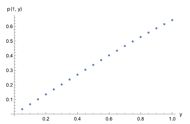
Figure 2. Numerical value of p(1, y) for $y=0.05, 0.10,\ldots,1$
.
$y=0.05, 0.10,\ldots,1$
.
The function p(x, 1) is also almost affine. We calculate $p(x,1) \approx 0.9844 - 0.3770 x$
for
$p(x,1) \approx 0.9844 - 0.3770 x$
for $0.05 \le x \le 1$
and
$0.05 \le x \le 1$
and $R^2 \approx$
96.15%. However, if we try a polynomial function of order 2 instead,
$R^2 \approx$
96.15%. However, if we try a polynomial function of order 2 instead, $R^2$
increases to 99.99%. The regression equation is
$R^2$
increases to 99.99%. The regression equation is
 \begin{equation*} p(x,1) \approx -0.003\,985 + 0.7152 x - 0.065\,59 x^2 \qquad \textrm{for}\ 0.05 \le x \le 1. \end{equation*}
Next, we deduce from [Reference Abramowitz and Stegun1, (10.4.59)] that
 \begin{equation} {\rm Ai}(z) \approx \frac{{\mathrm{e}}^{-({2}/{3}) z^{3/2}}}{2 \sqrt{\pi} z^{1/4}} \bigg(1- \frac{\Gamma(7/2)}{36 \Gamma(3/2)} z^{-3/2} \bigg) \approx \frac{{\mathrm{e}}^{-({2}/{3}) z^{3/2}}}{2 \sqrt{\pi} z^{1/4}} \big(1 - 0.104\,17 \, z^{-3/2}\big) \end{equation}
for $|z|$
large. Making use of this approximation, we find that the inverse Laplace transform of the function
$|z|$
large. Making use of this approximation, we find that the inverse Laplace transform of the function $L(y;\,\beta)$
given in (14) is
$L(y;\,\beta)$
given in (14) is
 \begin{align} p(x,y) \approx 1 + \frac{{\mathrm{e}}^{-({1}/{11}) {y^3}/{x}} x^{1/12}}{y^{7/4}} &\bigg\{{-}0.633\,98 \, {\rm CylinderD}\bigg({-}\frac{7}{6}, \frac{2 y^{3/2}}{3 \sqrt{x}\,}\bigg) y^{3/2} \nonumber \\ & \quad + 0.066\,04 \sqrt{x} \, {\rm CylinderD}\bigg({-}\frac{13}{6}, \frac{2 y^{3/2}}{3 \sqrt{x}\,}\bigg) \bigg\},\end{align}
where ${\rm CylinderD}(\nu,z)$
(in MAPLE) is the parabolic cylinder function denoted by
${\rm CylinderD}(\nu,z)$
(in MAPLE) is the parabolic cylinder function denoted by $D_{\nu}(z)$
in [Reference Abramowitz and Stegun1, p. 687].
$D_{\nu}(z)$
in [Reference Abramowitz and Stegun1, p. 687].
Remark 3. In theory, the approximation given in (15) is valid for $|z|$
large. However, as can be seen in Figure 3, it is quite accurate even in the interval [Reference Abramowitz and Stegun1, Reference Atkinson and Clifford4].
$|z|$
large. However, as can be seen in Figure 3, it is quite accurate even in the interval [Reference Abramowitz and Stegun1, Reference Atkinson and Clifford4].

Figure 3. Function ${\rm Ai}(y)$
(solid line) and its approximation (dashed line) given in (15) in the interval [Reference Abramowitz and Stegun1, Reference Atkinson and Clifford4].
${\rm Ai}(y)$
(solid line) and its approximation (dashed line) given in (15) in the interval [Reference Abramowitz and Stegun1, Reference Atkinson and Clifford4].
To check whether the formula for p(x, y) in (16) is precise, we numerically computed the inverse Laplace transform of the function $L(3;\,\beta)$
and compared it with the corresponding values obtained from (16) for
$L(3;\,\beta)$
and compared it with the corresponding values obtained from (16) for $x=0.5,1,\ldots,5$
. The results are presented in Table 1. We may conclude that the approximation is excellent (at least) when
$x=0.5,1,\ldots,5$
. The results are presented in Table 1. We may conclude that the approximation is excellent (at least) when $y=3$
.
$y=3$
.
Table 1. Probability p(x, 3) computed by numerically inverting the Laplace transform $L(3;\,\beta)$
(I), and the corresponding values obtained from (16) (II) for
$L(3;\,\beta)$
(I), and the corresponding values obtained from (16) (II) for $x=0.5,1,\ldots,5$
.
$x=0.5,1,\ldots,5$
.

2.2. Case 2
Suppose now that the process Y(t) has infinitesimal parameters $f(y) = \mu y$
and
$f(y) = \mu y$
and $v(y) = \sigma^2 y$
. If
$v(y) = \sigma^2 y$
. If $\mu < 0$
, Y(t) is a particular Cox–Ingersoll–Ross model (also called a CIR process). This is important in financial mathematics, in which it is used as a model for the evolution of interest rates.
$\mu < 0$
, Y(t) is a particular Cox–Ingersoll–Ross model (also called a CIR process). This is important in financial mathematics, in which it is used as a model for the evolution of interest rates.
Let $\Delta \,:\!=\, \sqrt{\mu^2 + 2 \beta \sigma^2}$
. The general solution of (10) with the above parameters is
$\Delta \,:\!=\, \sqrt{\mu^2 + 2 \beta \sigma^2}$
. The general solution of (10) with the above parameters is
 \begin{equation*} L(y;\,\beta) = c_1 \exp\bigg\{\frac{(-\mu + \Delta)}{\sigma^2} y\bigg\} + c_2 \exp\bigg\{\frac{(-\mu - \Delta)}{\sigma^2} y\bigg\} + \frac{1}{\beta}. \end{equation*}
In the case when $\mu=0$
,
$\mu=0$
, $\sigma=1$
, and
$\sigma=1$
, and $(a,b) = (0,\infty)$
, we find that the solution that satisfies the boundary conditions
$(a,b) = (0,\infty)$
, we find that the solution that satisfies the boundary conditions $L(0;\,\beta) = L(b;\,\beta) = 0$
, taking the limit as b tends to infinity, is
$L(0;\,\beta) = L(b;\,\beta) = 0$
, taking the limit as b tends to infinity, is $L(y;\,\beta) = ({1 - {\mathrm{e}}^{-\sqrt{2 \beta} y}})/{\beta}$
. This time, we are able to invert the Laplace transform analytically.
$L(y;\,\beta) = ({1 - {\mathrm{e}}^{-\sqrt{2 \beta} y}})/{\beta}$
. This time, we are able to invert the Laplace transform analytically.
Proposition 4.
For the diffusion process Y(t) with infinitesimal parameters $f(y) \equiv 0$
and
$f(y) \equiv 0$
and $v(y) = y$
, if
$v(y) = y$
, if $(a,b) = (0,\infty)$
, then the probability p(x, y) is given by
$(a,b) = (0,\infty)$
, then the probability p(x, y) is given by
 \begin{equation*} p(x,y) = {\rm erf}\bigg(\frac{y}{\sqrt{2 x}\,}\bigg), \end{equation*}
where ${\rm erf}(\cdot)$
is the error function defined by
${\rm erf}(\cdot)$
is the error function defined by ${\rm erf}(z) = ({2}/{\sqrt{\pi}}) \int_0^z {\mathrm{e}}^{-t^2} \, {\rm d} t$
.
${\rm erf}(z) = ({2}/{\sqrt{\pi}}) \int_0^z {\mathrm{e}}^{-t^2} \, {\rm d} t$
.
2.3. Case 3
Next, let Y(t) be an Ornstein–Uhlenbeck process, so that $f(y) = -\mu y$
, where
$f(y) = -\mu y$
, where $\mu>0$
, and
$\mu>0$
, and $v(y) \equiv \sigma^2$
. We find that the general solution of (10) is
$v(y) \equiv \sigma^2$
. We find that the general solution of (10) is
 \begin{align*} L(y;\,\beta) &= {\mathrm{e}}^{\beta y/ \mu} \bigg\{c_1 M\bigg({-}\frac{\sigma^2 \beta^2}{4 \mu^3},\frac{1}{2},\frac{\big(\sigma^2 \beta + \mu^2 y\big)^2}{\mu^3 \sigma^2} \bigg) \\ & \quad+ c_2 U\bigg({-}\frac{\sigma^2 \beta^2}{4 \mu^3},\frac{1}{2},\frac{\big(\sigma^2 \beta + \mu^2 y\big)^2}{\mu^3 \sigma^2} \bigg) \bigg\} + \frac{1}{\beta}, \end{align*}
where $M(\cdot,\cdot,\cdot)$
and
$M(\cdot,\cdot,\cdot)$
and $U(\cdot,\cdot,\cdot)$
are Kummer functions defined in [Reference Abramowitz and Stegun1, p. 504]. We can find the constants
$U(\cdot,\cdot,\cdot)$
are Kummer functions defined in [Reference Abramowitz and Stegun1, p. 504]. We can find the constants $c_1$
and
$c_1$
and $c_2$
for which
$c_2$
for which $L(a;\,\beta) = L(b;\,\beta) = 0$
. However, even in the simplest possible case, namely when
$L(a;\,\beta) = L(b;\,\beta) = 0$
. However, even in the simplest possible case, namely when $\mu=\sigma=1$
and
$\mu=\sigma=1$
and $(a,b)=(0,\infty)$
, it does not seem possible to invert the Laplace transform to obtain p(x, y). Proceeding as in Case 1, we could try to find approximate expressions for p(x, y).
$(a,b)=(0,\infty)$
, it does not seem possible to invert the Laplace transform to obtain p(x, y). Proceeding as in Case 1, we could try to find approximate expressions for p(x, y).
2.4. Case 4
Finally, if Y(t) is a geometric Brownian motion with $f(y) = \mu y$
and
$f(y) = \mu y$
and $v(y) = \sigma^2 y^2$
, the general solution of (10) is given by
$v(y) = \sigma^2 y^2$
, the general solution of (10) is given by
 \begin{equation*} L(y;\,\beta) = y^{{1}/{2}-{\mu}/{\sigma^2}} \bigg\{c_1 I_{\nu}\bigg(\frac{\sqrt{8 \beta y}}{\sigma} \bigg) + c_2 K_{\nu}\bigg(\frac{\sqrt{8 \beta y}}{\sigma} \bigg) \bigg\} + \frac{1}{\beta}, \end{equation*}
where $\nu = \big({2 \mu}/{\sigma^2}\big) - 1$
, and
$\nu = \big({2 \mu}/{\sigma^2}\big) - 1$
, and $I_{\nu}(\cdot)$
and
$I_{\nu}(\cdot)$
and $K_{\nu}(\cdot)$
are Bessel functions defined as follows [Reference Abramowitz and Stegun1, p. 375]):
$K_{\nu}(\cdot)$
are Bessel functions defined as follows [Reference Abramowitz and Stegun1, p. 375]):
 \begin{equation} I_{\nu}(z) = \bigg(\frac{z}{2}\bigg)^{\nu} \sum_{k=0}^{\infty} \frac{\big({z^2}/{4}\big)^{k}}{k! \Gamma(\nu+k+1)} , \qquad K_{\nu}(z) = \frac{\pi}{2} \frac{I_{-\nu}(z)-I_{\nu}(z)}{\sin(\nu \pi)}. \end{equation}
Because a geometric Brownian motion is always positive, we cannot set a equal to zero. We can nevertheless determine the constants $c_1$
and
$c_1$
and $c_2$
for
$c_2$
for $b > a >0$
and then take the limit as a decreases to zero. We can also choose
$b > a >0$
and then take the limit as a decreases to zero. We can also choose $a=1$
, for instance, and take the limit as b tends to infinity. For some values of the parameters
$a=1$
, for instance, and take the limit as b tends to infinity. For some values of the parameters $\mu$
and
$\mu$
and $\sigma$
, the function
$\sigma$
, the function $L(y;\,\beta)$
can be expressed in terms of elementary functions. Then, it is easier to evaluate the inverse Laplace transform numerically.
$L(y;\,\beta)$
can be expressed in terms of elementary functions. Then, it is easier to evaluate the inverse Laplace transform numerically.
3. Expected value of $\tau(x,y)$

We now turn to the problem of computing the expected value of the first-passage time $\tau(x,y)$
.
$\tau(x,y)$
.
Proposition 5.
The function $m(x,y)\,:\!=\,\mathbb{E}[\tau(x,y)]$
is a solution of the Kolmogorov backward equation
$m(x,y)\,:\!=\,\mathbb{E}[\tau(x,y)]$
is a solution of the Kolmogorov backward equation
 \begin{equation} \frac{1}{2} v(y) m_{yy}(x,y) + f(y) m_y(x,y) - y m_x(x,y) = -1. \end{equation}
The boundary conditions are
 \begin{equation} m(x,y) = 0 \quad if\ x=0,\ y=a\ or\ y=b. \end{equation}
Proof. Equation (18) is obtained (under appropriate assumptions) from the PDE (7) satisfied by the moment-generating function $M(x,y;\,\alpha)$
by first using the series expansion of the exponential function:
$M(x,y;\,\alpha)$
by first using the series expansion of the exponential function:
 \begin{align*} M(x,y;\,\alpha) \,:\!=\, \mathbb{E}\big[{\mathrm{e}}^{-\alpha \tau(x,y)}\big] & = \mathbb{E}\big[1 -\alpha\tau(x,y) + \tfrac{1}{2} \alpha^2 \tau^2(x,y) + \cdots\big] \\ & = 1 - \alpha \mathbb{E}[\tau(x,y)] + \tfrac{1}{2} \alpha^2 \mathbb{E}\big[\tau^2(x,y)\big] + \cdots \\ & = 1 - \alpha m(x,y) + \tfrac{1}{2} \alpha^2 \mathbb{E}\big[\tau^2(x,y)\big] + \cdots . \end{align*}
Then, substituting the above expression into (7), we indeed deduce that the function m(x, y) satisfies (18). Finally, since $\tau(0,y) = \tau(x,a) = \tau(x,b) = 0$
, we get the boundary conditions in (19).
$\tau(0,y) = \tau(x,a) = \tau(x,b) = 0$
, we get the boundary conditions in (19).
Remark 4.
-
(i) As in the case of the probability p(x, y), if
$Y(t) > a$
for
$t \ge 0$
, then we cannot write that
$m(x,a)=0$
for
$x>0$
. Actually, if
$a=0$
, we might have
$\lim_{y \downarrow 0} m(x,y) = \infty$
instead. -
(ii) Moreover, let A be the event
$\{Y(t) > a, \, 0 \le t \le \tau(x,y)\}$
. We may be interested in computing the mathematical expectation
$m^*(x,y) \,:\!=\, \mathbb{E}[\tau(x,y) \mid A]$
. That is, we want to compute the average time needed to leave the region
$\mathcal{C}$
, given that Y(t) will never be equal to a. In such a case, if Y(t) can indeed be equal to a, we would have the boundary condition
$m^*(x,a)= \infty$
.


If we assume that Y(t) can take on the values a and b, we can state the following proposition.
Proposition 6. The function
 \begin{equation} N(y;\,\beta) \,:\!=\, \int_0^{\infty} {\mathrm{e}}^{-\beta x} m(x,y) \, {\rm d} x \end{equation}
satisfies the non-homogeneous second-order linear ODE
 \begin{equation} \frac{1}{2} v(y) N''(y;\,\beta) + f(y) N'(y;\,\beta) - y \beta N(y;\,\beta) = -\frac{1}{\beta}. \end{equation}
Moreover, we have the boundary conditions
 \begin{equation} N(a;\,\beta) = N(b;\,\beta) = 0. \end{equation}
Proof. Equation (21) is deduced from the formula
 \begin{equation*} \int_0^{\infty} {\mathrm{e}}^{-\beta x} m_x(x,y) \, {\mathrm{d}} x = \beta \int_0^{\infty} {\mathrm{e}}^{-\beta x} m(x,y) \, {\mathrm{d}} x - m(0,y) \end{equation*}
and the boundary conditions in (19). Furthermore, (22) follows at once from (20) and (19).
We can obtain an explicit expression for the function $N(y;\,\beta)$
for all the cases considered in the previous section. However, in general it is difficult to calculate the inverse Laplace transform needed to get m(x, y). Therefore, we must either try to find an approximate solution, which can for instance be valid for large y, or invert the Laplace transform numerically in any particular case of interest.
$N(y;\,\beta)$
for all the cases considered in the previous section. However, in general it is difficult to calculate the inverse Laplace transform needed to get m(x, y). Therefore, we must either try to find an approximate solution, which can for instance be valid for large y, or invert the Laplace transform numerically in any particular case of interest.
We now present a problem where it is possible to compute m(x, y) explicitly and exactly. Consider the diffusion process Y(t) having infinitesimal mean $f(y)=1/y$
and infinitesimal variance
$f(y)=1/y$
and infinitesimal variance $v(y) \equiv 1$
, so that (21) becomes
$v(y) \equiv 1$
, so that (21) becomes
 \begin{equation} \frac{1}{2} N''(y;\,\beta) + \frac{1}{y} N'(y;\,\beta) - y \beta N(y;\,\beta) = -\frac{1}{\beta}. \end{equation}
Remark 5. The diffusion process Y(t) is a Bessel process of dimension 3. For this process, the origin is an entrance boundary [Reference Karlin and Taylor10, p. 239], which implies that if $Y(0)>0$
, then
$Y(0)>0$
, then $Y(t)>0$
for any
$Y(t)>0$
for any $t>0$
.
$t>0$
.
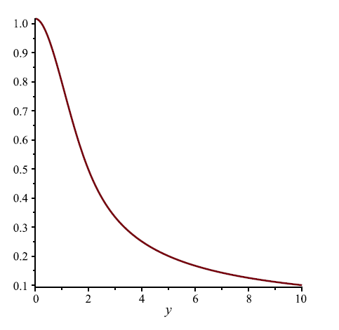
Figure 4. Function m(x, y) given in (24) when $x=1$
and
$x=1$
and $y \in (0,10)$
.
$y \in (0,10)$
.
The general solution of (23) is
 \begin{equation*} N(y;\,\beta) = \frac{1}{\sqrt{y}\,} \bigg\{c_1 I_{1/3}\bigg(\frac{2}{3} \sqrt{2 \beta} y^{3/2}\bigg) + c_2 K_{1/3}\bigg(\frac{2}{3} \sqrt{2 \beta} \, y^{3/2}\bigg)\bigg\} + \frac{1}{\beta^2 y}, \end{equation*}
where $I_{\nu}(\cdot)$
and
$I_{\nu}(\cdot)$
and $K_{\nu}(\cdot)$
are defined in (17). Moreover, suppose that
$K_{\nu}(\cdot)$
are defined in (17). Moreover, suppose that $(a,b)=(0,\infty)$
. Then, because
$(a,b)=(0,\infty)$
. Then, because $Y(t) \neq 0$
for
$Y(t) \neq 0$
for $t \ge 0$
, the function m(x, y) is actually the expected time taken by X(t) to hit the y-axis. We can show that the function
$t \ge 0$
, the function m(x, y) is actually the expected time taken by X(t) to hit the y-axis. We can show that the function $N(y;\,\beta)$
may be expressed as follows:
$N(y;\,\beta)$
may be expressed as follows:
 \begin{equation*} N(y;\,\beta) = -\frac{6^{1/6} \Gamma(2/3)}{\beta^{11/6} \pi \sqrt{y}} K_{1/3}\bigg(\frac{2}{3} \sqrt{2 \beta} y^{3/2}\bigg) + \frac{1}{\beta^2 y}. \end{equation*}
Now, it is indeed possible to invert the above Laplace transform. We find, with the help of MAPLE, that
 \begin{equation} m(x,y) = \frac{x}{y} - \frac{3^{7/6} \Gamma(2/3)}{4^{2/3} \pi} \frac{x^{4/3}}{y^2} {\mathrm{e}}^{-{y^3}/{9x}} W_{-{4}/{3},{1}/{6}}\bigg(\frac{2 y^{3}}{9 x}\bigg) \end{equation}
for $x>0$
and
$x>0$
and $y>0$
, where
$y>0$
, where $W_{\nu,\kappa}(\cdot)$
is a Whittaker function defined in [Reference Abramowitz and Stegun1, p. 505]. We can check that
$W_{\nu,\kappa}(\cdot)$
is a Whittaker function defined in [Reference Abramowitz and Stegun1, p. 505]. We can check that $\lim_{x \downarrow 0} m(x,y) = 0$
(as required) and that
$\lim_{x \downarrow 0} m(x,y) = 0$
(as required) and that $\lim_{y \rightarrow \infty} m(x,y) = 0$
, which follows from the definition of X(t):
$\lim_{y \rightarrow \infty} m(x,y) = 0$
, which follows from the definition of X(t): ${\mathrm{d}} X(t) = -Y(t) \, {\mathrm{d}} t$
. Finally, we compute
${\mathrm{d}} X(t) = -Y(t) \, {\mathrm{d}} t$
. Finally, we compute
 \begin{equation*} \lim_{y \downarrow 0} m(x,y) = \frac{3^{11/6} \Gamma(2/3)}{2^{5/3} \, \pi} \, x^{2/3}.\end{equation*}
The function m(1, y) is shown in Figure 4 for $y \in (0,10)$
. Furthermore, the same function is presented in Figure 5 for
$y \in (0,10)$
. Furthermore, the same function is presented in Figure 5 for $y \in (0,0.05)$
in order to show the convergence of the function as y decreases to zero.
$y \in (0,0.05)$
in order to show the convergence of the function as y decreases to zero.

Figure 5. Function m(x, y) given in (24) when $x=1$
and
$x=1$
and $y \in (0,0.05)$
.
$y \in (0,0.05)$
.
4. Moment-generating function of
$\tau(x,y)$

As we have seen in Section 2, the moment-generating function $M(x,y;\,\alpha)$
of
$M(x,y;\,\alpha)$
of $\tau(x,y)$
satisfies the Kolmogorov backward equation
$\tau(x,y)$
satisfies the Kolmogorov backward equation
 \begin{equation*} \tfrac{1}{2} v(y) M_{yy}(x,y;\,\alpha) + f(y) M_y(x,y;\,\alpha) - y M_x(x,y;\,\alpha) = \alpha M(x,y;\,\alpha). \end{equation*}
This PDE is subject to the boundary conditions in (8).
Remark 6. Let $M^*(x,y;\,\alpha) \,:\!=\, \mathbb{E}[{\mathrm{e}}^{-\alpha \tau(x,y)} \mid X(\tau(x,y)) = 0]$
. This function satisfies (7), subject to the boundary conditions
$M^*(x,y;\,\alpha) \,:\!=\, \mathbb{E}[{\mathrm{e}}^{-\alpha \tau(x,y)} \mid X(\tau(x,y)) = 0]$
. This function satisfies (7), subject to the boundary conditions
 \begin{equation*} M^*(x,y;\,\alpha) = \left\{ \begin{array}{c@{\quad}l} 1 & \textrm{if}\ x=0\ \textrm{and}\ a < y < b, \\[3pt] 0 & \textrm{if}\ y=a\ \mathrm{or}\ y=b\ \textrm{and}\ x>0. \end{array} \right. \end{equation*}
Similarly,
 \begin{equation} M^{**}(x,y;\,\alpha) \,:\!=\, \mathbb{E}[{\mathrm{e}}^{-\alpha \tau(x,y)} \mid Y(\tau(x,y)) = a \; {\rm or} \; Y(\tau(x,y))=b] \end{equation}
satisfies (7) as well, and the boundary conditions are
 \begin{equation*} M^{**}(x,y;\,\alpha) = \left\{ \begin{array}{c@{\quad}l} 0 & \textrm{if}\ x=0\ \textrm{and}\ a < y < b, \\[4pt] 1 & \textrm{if}\ y=a\ \mathrm{or}\ y=b\ \textrm{and}\ x>0. \end{array} \right. \end{equation*}
We define the Laplace transform
 \begin{equation} \Phi(y;\,\alpha,\beta) = \int_0^{\infty} {\mathrm{e}}^{-\beta x} M(x,y;\,\alpha) \, {\mathrm{d}} x. \end{equation}
Since
 \begin{equation*} \int_0^{\infty} {\mathrm{e}}^{-\beta x} M_x(x,y;\,\alpha) \, {\mathrm{d}} x = \beta \int_0^{\infty} {\mathrm{e}}^{-\beta x} M(x,y;\,\alpha) \, {\mathrm{d}} x - M(0,y;\,\alpha),\end{equation*}
we can prove the following proposition.
Proposition 7.
The function $\Phi(y;\,\alpha,\beta)$
defined in (26) satisfies the non-homogeneous second-order linear ODE
$\Phi(y;\,\alpha,\beta)$
defined in (26) satisfies the non-homogeneous second-order linear ODE
 \begin{equation} \tfrac{1}{2} v(y) \Phi''(y;\,\alpha,\beta) + f(y) \Phi'(y;\,\alpha,\beta) - y [\beta \Phi(y;\,\alpha,\beta)-1] = \alpha \Phi(y;\,\alpha,\beta). \end{equation}
If Y(t) can take on the values a and b, the boundary conditions are
 \begin{equation} \Phi(a;\,\alpha,\beta) = \Phi(b;\,\alpha,\beta) = \frac{1}{\beta}. \end{equation}
Remark 7. Because the moment-generating function $M(x,y;\,\alpha)$
is itself a Laplace transform,
$M(x,y;\,\alpha)$
is itself a Laplace transform, $\Phi(y;\,\alpha,\beta)$
is a double Laplace transform.
$\Phi(y;\,\alpha,\beta)$
is a double Laplace transform.
Although it is possible to find the solution to (27) that satisfies the boundary conditions in (28) for the most important diffusion processes, the expressions obtained are quite complex. Therefore, inverting the Laplace transform to get the moment-generating function $M(x,y;\,\alpha)$
is generally very difficult.
$M(x,y;\,\alpha)$
is generally very difficult.
The function $\Psi(y;\,\alpha,\beta) \,:\!=\, \int_0^{\infty} {\mathrm{e}}^{-\beta x} M^{**}(x,y;\,\alpha) \, {\mathrm{d}} x$
, where
$\Psi(y;\,\alpha,\beta) \,:\!=\, \int_0^{\infty} {\mathrm{e}}^{-\beta x} M^{**}(x,y;\,\alpha) \, {\mathrm{d}} x$
, where $M^{**}(x,y;\,\alpha)$
is defined in (25), satisfies the homogeneous ODE
$M^{**}(x,y;\,\alpha)$
is defined in (25), satisfies the homogeneous ODE
 \begin{equation*} \tfrac{1}{2} v(y) \Psi''(y;\,\alpha,\beta) + f(y) \Psi'(y;\,\alpha,\beta) - y [\beta \Psi(y;\,\alpha,\beta)-0] = \alpha \Psi(y;\,\alpha,\beta). \end{equation*}
Suppose that Y(t) is a standard Brownian motion and that $(a,b)=(0,\infty)$
. We must then solve
$(a,b)=(0,\infty)$
. We must then solve $\frac{1}{2} \Psi''(y;\,\alpha,\beta) = (\alpha + \beta y) \Psi(y;\,\alpha,\beta)$
, subject to
$\frac{1}{2} \Psi''(y;\,\alpha,\beta) = (\alpha + \beta y) \Psi(y;\,\alpha,\beta)$
, subject to $\Psi(0;\,\alpha,\beta) = 1/\beta$
. We find that
$\Psi(0;\,\alpha,\beta) = 1/\beta$
. We find that
 \begin{equation*} \Psi(y;\,\alpha,\beta) = \frac{{\rm Ai}\big({2^{1/3} (\alpha + \beta y)}/{\beta^{2/3}}\big)}{\beta {\rm Ai}\big({2^{1/3} \alpha}/{\beta^{2/3}}\big)} \qquad \textrm{for}\ y \ge 0. \end{equation*}
It is not difficult to invert the Laplace transform numerically for any values of $\alpha$
and y.
$\alpha$
and y.
5. Concluding remarks
Solving first-passage problems for integrated diffusion processes is a difficult task. In this paper, we were able to obtain explicit solutions to such problems for the most important diffusion processes. In some cases, the solutions were exact ones. We also presented approximate solutions. When it was not possible to give an analytical expression for the function we were looking for, we could at least use numerical methods in any special case.
As mentioned in the introduction, the author has used integrated diffusion processes in optimal control problems. These processes can serve as models in various applications. In particular, if ${\mathrm{d}} X(t) = k Y(t) \, {\mathrm{d}} t$
, X(t) can represent the wear (if
${\mathrm{d}} X(t) = k Y(t) \, {\mathrm{d}} t$
, X(t) can represent the wear (if $k > 0$
) or the remaining amount of deterioration (if
$k > 0$
) or the remaining amount of deterioration (if $k < 0$
) of a machine when Y(t) is always positive, so that X(t) is strictly increasing (or decreasing), which is realistic.
$k < 0$
) of a machine when Y(t) is always positive, so that X(t) is strictly increasing (or decreasing), which is realistic.
Finally, we could generalise the results presented in this paper by assuming that X(t) is a function of one or more independent diffusion processes $Y_1(t),\ldots,Y_i(t)$
, as for the wear processes defined in [Reference Rishel17]. In the case of the application to the degradation of a marine wind turbine, environmental variables that influence its wear are, in addition to wind speed, air temperature, humidity, salinity, etc.
$Y_1(t),\ldots,Y_i(t)$
, as for the wear processes defined in [Reference Rishel17]. In the case of the application to the degradation of a marine wind turbine, environmental variables that influence its wear are, in addition to wind speed, air temperature, humidity, salinity, etc.
Of course, if we consider at least two such variables, the problem of computing the function $p(x,y_1,\ldots,y_i)$
that generalises p(x, y), for example, becomes even harder, because taking the Laplace transform of this function with respect to x will not transform the Kolmogorov backward equation, which is a partial differential equation, into an ordinary differential equation.
$p(x,y_1,\ldots,y_i)$
that generalises p(x, y), for example, becomes even harder, because taking the Laplace transform of this function with respect to x will not transform the Kolmogorov backward equation, which is a partial differential equation, into an ordinary differential equation.
In some cases, it might be possible to exploit the symmetry present in the problem to reduce the PDE to an ODE. That is, we might make use of the method of similarity solutions to express the Laplace transform $L(y_1,y_2;\,\beta)$
of the function
$L(y_1,y_2;\,\beta)$
of the function $p(x,y_1,y_2)$
as a function
$p(x,y_1,y_2)$
as a function $L^*(z;\,\beta)$
, where z is the similarity variable. For instance, in some problems
$L^*(z;\,\beta)$
, where z is the similarity variable. For instance, in some problems $L(y_1,y_2;\,\beta)$
could be a function of
$L(y_1,y_2;\,\beta)$
could be a function of $z \,:\!=\, y_1+y_2$
, thus transforming the PDE it satisfies into an ODE. For this method to work, both the PDE (after simplification) and the boundary conditions must be expressible in terms of the variable z.
$z \,:\!=\, y_1+y_2$
, thus transforming the PDE it satisfies into an ODE. For this method to work, both the PDE (after simplification) and the boundary conditions must be expressible in terms of the variable z.
Acknowledgement
The author wishes to thank the anonymous reviewers of this paper for their constructive comments.
Funding information
This research was supported by the Natural Sciences and Engineering Research Council of Canada (NSERC).
Competing interests
There were no competing interests to declare which arose during the preparation or publication process of this article.


