1. The problem

Tn this paper we outline a problem concerned with the movement and large-scale deformation of pack ice and show how photographs taken by the Earth Resources Technology Satellite (ERTS) help to solve it. The problem arises from the Arctic. lee Dynamics Joint Experiment (AIDJEX) (Untersteiner, 1974). In the main experiment, due to take place from March 1975 to April 1976 in the Beaufort Sea, a roughly circular area of sea ice, 400 km in radius, will be chosen. The distribution of the varying forces from the wind on the upper surface of the ice and from the ocean on the lower surface, which are the main driving forces, will be determined over this area and the movement of the outer boundary will also be measured. With information on the initial state of the ice (in fact a histogram of the ice thicknesses present in each elementary area) it should, in principle, be possible to predict the details of the motion of the ice within the boundary, and to compare the predictions with additional observations of the motion. To make a satisfactory prediction it is essential to take into account the mechanical interaction between neighbouring areas of ice. The AIDJEX modelling group propose to adopt a two-dimensional continuum model of the ice pack and to specify the constitutive law that governs its mechanical behaviour. The present working hypothesis (Reference Coon, Coon, Maykut, Pritchard, Rothrock and ThorndikeCoon and others, 1974) is that the pack ice has an elastic -plastic constitutive law. The study to be described here used ERTS photography first of alt to test whether on some scale or scales the pack ice can indeed be modelled as a two-dimensional continuum. This postulate is fundamental to the AIDJEX model; the idea is that although on a small scale there are discontinuities, such as the formation of open leads and pressure ridges, these will average out over a large enough scale so that the deformation approximates to that of a continuum—just as in engineering, for example, classical elasticity is a good model on scales much larger than the spacing between atoms. The potential difficulty with this idea is that when the scale becomes very large, say several hundreds of kilometres, the driving forces from wind and water can no longer be considered as uniform. The hope is that the deformation can be modelled as continuous before such a large scale is reached. In principle, the postulate could be true or false. (These are extremes; in intermediate cases the continuum model would represent the ice behaviour more or less well.) For example, if the individual ice noes are small enough the postulate will be true; on the other hand, if the floes all behaved rigidly and were so large that a completely different average wind acted on each one, there would be no scale where a continuum model would work and the postulate would be false.

2. The use of erts photographs

ERTS photographs have already been used by Reference Crowder, Crowder, McKim, Ackley, Hibler, Anderson, Santeford and SmithCrowder and others (1974), Hibler and others (in press), Shapiro and Burns (in press), and Reference Barnes and BowleyBarnes and Bowley (1974) to study the movement of sea ice. They are ideally suited to studying the questions raised above, for they contain all the spatial detail that is needed. Figure ta shows part of the ice pack in the Beaufort Sea in May [973, and Figure lb shows its appearance 17 d later. The same ice features such as the floes marked p and Q can be seen in both. The correspondence between details is much more readily seen when two positive transparencies are superimposed. Since the ERTS pictures are essentially maps on a scale of 1: 10⁶ with very little distortion (the distortion error, about 70 m, is in fact about the same as the resolving power of the system), the readily measurable lack of register between corresponding features is virtually entirely due to deformation of the ice pack.

Figure 2 shows the relative motion of eight points in the ice that are visible in the two pictures. They are joined in arbitrary pairs by straight lines. The eight points for 7 May (joined by full lines) are superimposed on the corresponding eight points for 24 May (joined by broken lines) by making points O on floe p coincide and then rotating the pictures relative to one another for the best fit. The lack of register that remains, as seen in Figure 2, is a measure of the strain. One can see that there has been an extension north-south of some 6% in 17 d (0.4% d^-1). East-west there has been a compression ranging from 8% (0.5% d^-1) at the south end of the figure to zero at the north end.

Floe P in Figure 1a, b shows measurable deformation, but in floe Q, which is 80 km long. although there are visible changes in its edges, there is no measurable overall distortion (±2%, or 0.1% d^-1). Thus, in this case, a continuum model of the deformation would presumably not be appropriate on a scale of 80 km. The problem here is not in the remote sensing, which has ample accuracy, but is inherent in the behaviour of the sea ice itself.

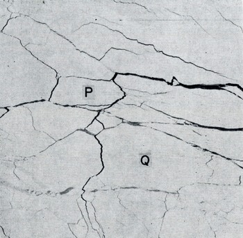
Fig. 1a. Arctic sea ice on 7 May 1973 (lat. 78°N., long. 126° W.). ERTS photograph no. E-1288-21151-5.

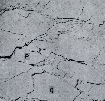
Fig. 1b. Approximately the same area as Figure 1a on 24 May 1973. ERTS photograph no. E-1305-21092-5.

Further examples show that on scales rather greater than this, a continuum model can be applied, but before describing these we must discuss the problem of measuring displacement from ERTS pictures, as distinct from measuring strain. In so-called “bulk imagery“, which is what was available for this area, the individual frames have latitude and longitude ticks at their edges. If successive frames in the same orbit are registered by the details they have in common (the operation of the scanner in the satellite means that these are actually the same data, but possibly corrected slightly differently for each frame) so as to form a strip, the latitude and longitude ticks on the different frames disagree typically by 2 km. 1 or 2 km seems to be the accuracy with which the absolute position of a feature can be determined. Cartographers improve on this by a factor of 10 or more, up to the limit of resolution of the system, by using ground control. At sea, one cannot normally do this unless a strip of usable photographs crosses a coast-line, which is not often the case. Thus, by seeing the same ice feature on two separate occasions, we can measure its absolute displacement to within i or 2 km. During the AIDJEX main experiment, however, it ought to be possible to improve this to too rn by making use of the manned camps on the ice and the data buoys which will be in operation. We shall call these prime points. The positions of prime points will be known from satellite observations using the Doppler effect to probably better than 100 m, and strips of ERTS pictures will not infrequently include one or more prime points. However, unlike the usual requirement for ground control, no ground marking of the prime points is needed, for in this application it is not necessary to identify the exact position of a prime point on the ERTS photograph. The changing position data from a prime point tell us its displacement to within 100 m, and so we know that some point on the ERTS image within a 2 km circle has that displacement. We can now assume that the nearest identifiable ice feature (say, within a few kilometres) has that same displacement. This tells us how we must superimpose the two ERTS images at that point, and so removes the I km or 2 km systematic error in displacement at that point. The method works because, although 2 km is an uncomfortably large error in displacement, it is of little importance as an error in the absolute position where the displacement is measured. An uncertainty will still remain corresponding to a relative rotation of the two pictures about the prime point. This uncertainty is removed if the strip of ERTS pictures contains two prime points, and then the displacement can be determined throughout the overlap region to within 100 m.

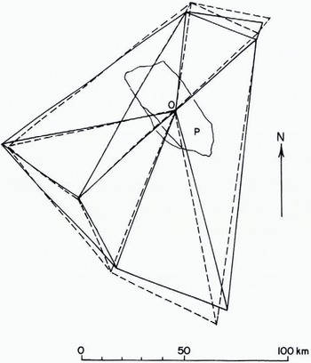
Fig. 2. Drawn from Figures 1a and b to show the distortion of the ice over a 17 d period.

Whether or not the strip of ERTS pictures contains a prime point, the relative displacements of points on the same strip can be measured to within 100 to 200 m, except for an uncertainly in rotation. Thus, on a gauge length of 100 km, strain can be measured with an accuracy of 0.1% strain.

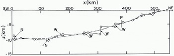
Fig. 3a. The variation of it, the x component of displacement, with distance x along a line. Period 21 to 23 March 1973-From ERTS photographs no. E-1241-21571-5,64-5, 62-5, 55-5, 53-5; E-1243-22084-5, 81-5, 75-5, 72-5, 70-5.

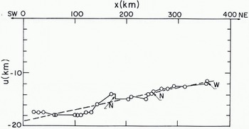
Fig. 3b. As for Figure 3a, but for a different area later in the year {14-16 June 1973). From ERTS photographs no. E-1326-21273-5, 70-5, 64-5; E-1328-21383-5, 81-5, 74-5.

Figure 3 shows the results of displacement measurements along lines several hundred kilometres long. To construct Figure 3a five successive ERTS frames for 21 March 1973 were joined together so that the overlapping ice detail was in register. The strip so formed was superimposed on a corresponding strip for 23 March 1973 by making the latitude and longitude lines coincide so far as possible. An x-axis, 500 km long, was drawn down the centre of the overlap region and the displacement over two days of ice points initially on the Λ-axis was measured. Figure 3a shows the x-component, u, plotted against x. A series of zigzagging leads, each a few kilometres wide, spaced at distances between 10 km and 60 km provided nearly all the measurement points. In some cases measurable movement, widening (w) or narrowing (N), took place on them; the u: x graph is nearly vertical at these places. On other segments of the measurement line, strain occurred without any active leads or ridges being visible. Figure 3a shows a general trend (broken line) of «increasing with x, that is, stretching; u changes from —9.6 km 10 zero over a distance of 500 km, while the stretching rate increases from 0.0% d^-1 at the left (SW) to 1.9% d^-1 at the right (NE). Superimposed on this general trend there are spatial fluctuations of u which give rise to a mean absolute deviation from the broken line of 0.43 km. Thus, on the left, the small-scale variations in velocity are 4.5% of the total velocity. The uncertainties in latitude and longitude introduce in this case a uniform systematic error of 1 or 2 km in u.

Figure 3b shows the result of similar measurements three months later in the season (14-16 June 1973) at a place where the floe size was considerably smaller. The general trend is here adequately represented by a straight line (the broken line). In this case the small-scale variations in velocity are still about 4% of the total, in spite of the smaller floe size.

3. Conclusions

The general feature of Figure 3, and of a third set of measurements not reported here, is that there is a spatial variation of ice velocity on a scale of several hundreds of kilometres; smaller-scale variations of velocity are superimposed on this, but their amplitude is not enough to obscure the large-scale trend. If these examples are representative (and we have no reason to suppose they are not) we can conclude that it is justifiable to adopt a continuum model. A scale of 100 km would be reasonable for measuring the large-scale trend. There is ample accuracy in the measurements from the ERTS pictures, but the inherent graininess of the ice limits the application of a continuum model; specifically, it would not be meaningful to specify continuum strain-rates on a scale of 100 km to more than a certain accuracy. In one sense, this could be thought of as the uncertainty in the slope of the smoothed (broken) curves in Figure 3. In that case we should be concerned with averaging the slopes of the true (full) curve in a one-dimensional fashion, since the only information used is along one line, namely the *-axis. However, to obtain the smoothed curve one should really take averages two-dimensionally and this will reduce the uncertainty in the slope. The resulting imprecision in the continuum strain-rate on a scale of 100 km has not yet been calculated, but it seems likely that it is of the order of 0.1% d^-1. It could readily be obtained by first making measurements of displacement components (u, v) at a number of different points within, say, a too km X 100 km square, and then fitting the results, by a least-squares method, to a linear variation of u and v with respect to x and y. By this means one could find the average displacement (two quantities) and the average deformation (four quantities) within the area, together with their uncertainties. The average deformation may then be expressed as the principal strains, their azimuth, and the rotation.

The work described was a preliminary study. It suggests that measurements of displacement and deformation for comparison with the predictions of a continuum model can be readily obtained if ERTS pictures are available. At the time of writing ERTS-i is reaching the end of its useful life and ERTS-B is expected to be launched early in 1975 in time for the AIDJEX main experiment.

A full report of this study, including an estimate of the amount of cloud-free coverage likely to be available during the main experiment and a discussion of the use of aircraft photography as an alternative to ERTS, is given in Nye and Thomas (1974). The work was done while I was a visitor to the AIDJEX office. I am indebted to Mr D. R. Thomas for making the measurements on which Figure 3 is based, and to other members of the AIDJEX staff for their willing assistance.