


Nomenclature

Introduction
The discovery of oil on the Northern Slope of Alaska has raised many questions concerning the effects of oil spills in the Arctic Ocean and other ice-filled waters. The handling and transporting of oil in sizable quantities always results in some spillage, the average spillage being on the order of 0.1% of the quantity transported (Reference Blumer and HoultBlumer, 1969, p. 6). The North Slope borders on the Arctic Ocean which is essentially ice-locked for about nine months of the year (Reference HanoverAnonymous, 1970, p. 11). Even during the summer months the permanent ice cover remains within ten nautical miles (18 km) of the shore (Reference HanoverAnonymous, 1970, p. 34). Any sort of water-born transport of North Slope crude oil will create the possibility of spilling large amounts of crude oil under the ice.
Granted that under-ice oil spills are almost certain to occur if Arctic oil operations continue, it is important to know how such spills can be contained and removed if the environmental damage caused by them would be serious enough to warrant such action. In the search for this information, the first question to ask is how the oil spill behaves under the ice. Much is known of how oil spreads on temperate waters, both from experimental and theoretical studies and from observations of large-scale disasters such as the Torrey Canyon and Santa Barbara Channel incidents. Almost nothing is known of the behavior of an oil spill under sea ice. The speed with which the oil spreads or the ultimate thickness to which it spreads are unknown. The interaction between the oil and the peculiar microstructure of the lower layer of the sea ice (see Reference Weeks and CurrieWeeks, 1968, p. 137–78) is also unknown.
There has been a good deal of speculation concerning the way sea ice will interact with oil trapped under it. Three principal modes of behavior have been considered possible: (1) The sea ice will entrap the oil causing the formation of a matrix of oil and ice; (2) the ice will entrap the oil in a pool and proceed to form beneath it; (3) the ice will continue to grow pushing the oil before it (see Fig. 1). Such a phenomenon is difficult to observe in field experiments, so laboratory experiments were conducted to determine which of these phenomena occurred and to examine the phenomenon quantitatively, if possible.

Fig. 1. Possible modes of oil entrapment.
These experiments were set up and run using the two oils most likely to be spilled in the Arctic: North Slope crude and diesel fuel. No attempt has been made to extrapolate the data to other oils. The present tests give results which would be appropriate for spills of these two oils.
Experimental Apparatus and Methods
The principal function of the laboratory apparatus was to produce a nearly uniform vertical heat flux in a tank of sea-water. The apparatus consisted of a 1.59 cm (


Fig. 2. Schematic diagram of sea-ice test cell.
The quantities measured during the experiments were the temperature distribution in the ice and water, the salinity of the water beneath the ice, the depth of growth of the ice, and the amount of oil injected under the ice. Temperature was measured with a bridge of copper-constantan thermocouples. The salinity of the water beneath the ice was measured by the use of a specially designed, totally submerged hydrometer. The depth of growth of the ice was determined by measuring the depth as seen through the tank with a scale. The growth velocity of the ice was computed by noting the time that each thickness measurement was made and calculating the arithmetic mean velocity between successive measurements.
As a substitute for sea-water, solar sea salt was dissolved in tap water until a salinity of approximately 3‰ was achieved. This was used at the start of each experiment, but salt rejection by the ice increased the salinity of the water to between 35 and 40‰ by the time oil was placed under it. Two types of oil were used. No. 2 diesel was chosen because it is readily available and because it is a common marine fuel which may be subject to large-scale spills. The other oil used was a North Slope crude oil.
Each experiment was started with an initial plate temperature of −29° C until a few centimeters of ice formed. Then the temperature was set to the temperature at which the experiment was to run. When the ice reached a depth between 12 and 16 cm, oil was injected through the bottom of the tank from a plenum chamber using compressed air to supply the driving pressure. Except in a few trial runs, enough oil was added to completely cover the lower surface of the ice. The average thickness of the oil layer ranged between 1 and 2.6 cm. The oil was allowed to remain until some ice began to form on its lower surface. This took 12–24 h in most cases. The experiment was then terminated and the ice block removed.
In order to determine the extent to which oil became entrapped in the ice or adhered to its lower surface, the lowermost 2.5 cm of the ice block was sawed off, and the slab of ice was melted. The dimensions of the slab were noted before melting. The oil and water obtained were collected in a graduated cylinder and measured. Because the technique for measurement of the adhering oil is so crude, the limits of uncertainty for these data are rather wide.
Since the porosity of sea ice increases markedly at temperatures near the melting point, an attempt was made to see if there was any marked change in the mode of oil entrapment as the ice melts. The existing apparatus could not actually simulate the melting of sea ice as it occurs in the ocean because the tank had a finite heat gain from the laboratory; there is no similar source of heat in the sea. Nevertheless the experiment was conducted. After the completion of an experiment performed in the usual manner, the temperature of the cold plate was raised to −1.4° C, and the ice was allowed to melt. Temperature profiles were recorded every two hours and visual observations of the ice were made.
A more detailed description of the experimental apparatus methods is available in Wolfe (unpublished, p. 14–22).
Experimental Observations and Results
Sea-ice growth rate
A steady-state approximation to the flow of heat from the sea-water to the cold plate may be used. The rate of formation of ice is set equal to the rate of heat flux divided by the heat of formation of the ice:

Since the thermal conductivity of the ice is essentially constant over the range of temperature encountered, and the flow of heat is uniform upwards, the temperature gradient in the ice is constant. Since the cold ice surface is at the top of the sea-water, the “sea” is well mixed and of uniform temperature approximately equal to the liquidus temperature of a solution of NaCl and water with concentration 35‰.
The temperature data can be put in dimensionless form and normalized by dividing the temperature difference between the local temperature and the water temperature by the total temperature difference between the water and the cold plate:

Distance is normalized by measuring the distance Z from the lower surface of the ice to the thermocouple and dividing this by the total thickness of the ice:

All of the temperature data obtained before the addition of the oil are shown plotted in this manner in Figure 3. It demonstrates that, within the limits of experimental error, the temperature gradients are uniform and that the resistance of the thermal boundary layer at the ice-water interface is negligible.
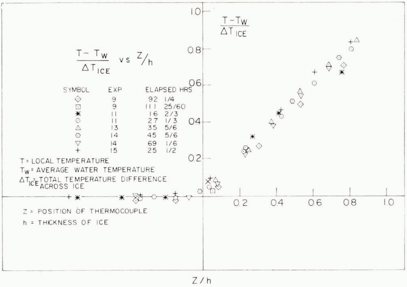
Fig. 3. Dimensionless temperature profiles.
The heat flow from the warm laboratory to the test cell retards the rate of formation of ice below that predicted by Equation (1) above. The rate of heat gain by the ice tank from the laboratory should be nearly constant for all growth conditions, and thus the rate of formation should approach that given by Equation (1) for high rates of growth. The available temperature and growth-rate data may be made dimensionless and normalized by dividing the product of the heat of formation of ice and the measured growth rate. ρLV, by the heat flux out through the ice as predicted by Equation (2)

This dimensionless growth rate is plotted as a function of ρLV divided by the calculated heat gain per unit area through the walls of the tank and is displayed in Figure 4. Note that the value of the dimensionless parameter ρLV/[k (∆T)/h] drops noticeably below unity when the ratio ρLV/(Q gain/A) is about 150/1. The area of the tank walls is about 15 times the area of the cold plate. As expected, the growth velocity deviates significantly from Equation (1) when the ratio of ρLV to the total heat gain is about 1/10. The large error bars on each data point are due primarily to the large uncertainty in the measurement of the rate of growth.

Fig. 4. Dimensionless growth velocity to heat flux ratio as a/unction rif growth velocity to heat gain ratio.
Mode of oil entrapment
The actual method by which the crude and diesel oils are trapped in the sea ice is a combination of modes (a) and (c) shown in Figure 1. The bulk of the oil is pocketed in a pool below the original ice sub-surface while more sea ice proceeds to grow under it. A small amount of oil does rise into the pores of the skeletal layer, and into small, vertical shafts which rise from the lower surface of the ice. These shafts may be air bubbles similar to those that form in fresh water ice due to the inability of air entrained in the water and rejected upon freezing to escape beyond the advancing ice front (Reference Assur and WeeksWeeks and Assur, 1969, p. 8). The total amount of oil contained in these air bubbles is small in comparison with the amount of oil that adheres to the lowermost inch (couple of centimetres) of the ice (see below). During the ice melting experiment, a considerably greater amount of oil rose into the ice, especially into the air shafts. In some instances it reached as high as 8 cm above the lower surface of a 13 cm thick block, yet the volume of oil trapped in this manner was still small, amounting to no more than 1/150 of the volume of the ice.
The presence of the oil pool has a significant effect upon the heat transfer through the ice. The simple model of heat transfer through sea ice described above assumes a uniform solid of constant conductivity between two constant temperature regions, one at the liquidus temperature of sea-water and the other at the ambient temperature of the air, or in the experimental case, the cold plate. As the oil has a thermal conductivity that is considerably lower than that of the ice, its presence acts as an insulating layer, impeding the flow of heat and reducing the temperature drop across the ice.
The temperature data obtained after the oil was placed under the ice may be made dimensionless in the same manner as was done for the data taken with ice only. The origin for the vertical axis remains at the lower surface of the original ice block. As a result temperature measurements in the oil and below are expressed as negative numbers. The thickness of the ice before the oil was added is used to normalize distance, but the total temperature drop across the ice and oil is used to normalize temperature. The normalized temperature distributions are shown plotted in Figure 5 for all temperature measurements taken after the oil was in place.
As can be seen in Figure 5, the temperature profile in the ice is linear at all times after the addition of the oil except for the case of experiment 9, in which the temperature of the plate was high enough that the heat gain by the tank caused the water temperature to rise continuously. In the four other cases in which temperature profiles were measured, the temperature gradient in the ice remained constant, but decreased in magnitude from its initial values as shown in Figure 3 through intermediate values to the final value. The temperature distribution in the oil could not be determined directly, since the oil layer was between 1.3 and 2.5 cm thick and the thermocouples were spaced 2.54 cm (one inch) apart in the bridge. It is clear that temperature gradients in the oil were much larger than in the ice.

Fig. 5. Dimensionless temperature profiles after oil insertion.
Whereas, clearly, the heat transfer through the ice is that of solid body conduction, the mode of heat transfer in the oil pool is not obvious. It should be noted in Figure 5 that, for all of the crude oil experiments, the ratio of the temperature drop across the oil to that across the oil and ice is the same, 0.6. This ratio is independent of the thickness of the oil pool, which varies between 1.3 and 2.5 cm (in dimensionless form, (z/h), −0.097 and −0.189). For the diesel oil the ratio of the temperature drop across the oil to the total temperature drop across the oil and ice is 0.3. This behavior is not in accordance with the theory of static heat conduction. The thermal conductivity of most petroleum distillates is only a very weak function of temperature, and over the range of temperatures considered, the thermal conductivity of the liquid fractions of petroleum changes less than 3%. (Wolfe, unpublished, appendix I). Within the limits of precision of this experiment, it may be considered constant. For constant thermal conductivity, the thermal resistance of a solid conducting heat in one direction is h/k, and thus the temperature drop across the solid is proportional to its thickness. For two solids conducting in series, the ratio of the temperature drop across one to the temperature drop across the other is (h 1/h 2) (k 2/k l). This is clearly not the case for the ice block and oil pool.
It is therefore not proper to assume that the mode of heat transfer in the oil pool is by conduction alone. At the temperature involved, the crude oil is indeed highly viscous, but further examination is necessary to determine if it may be considered a solid body. The diesel fuel is quite fluid; it is entirely possible that convection cells could form and reduce the thermal resistance of the oil layer below that predicted by static conduction theory. The Nusselt number is the dimensionless ratio of the convective heat transfer coefficient K to the conductive heat transfer coefficient k/h. For free convection between plane, horizontal surfaces, the Nusselt number may be defined as

The Nusselt modulus can be shown to be a function of the Grashof number and the Prandtl number, defined by relations,


provided that the mode of heat transfer is free convection only (Reference KreithKreith, 1965, p. 333). When a normal fluid whose density decreases with increasing temperature is placed between plane surfaces and cooled from above, convection results. This convection is commonly described in terms of the Rayleigh number which is the product of the Grashof and Prandtl numbers, (Gr) (Pr). When this dimensionless variable is less than about 1 700, no convection results, and heat is transferred by static conduction only. When (Gr)(Pr) is between 1 700 and 42 000 convection is in the peculiar cellular manner known as Bénard cell convection. Irregular turbulence results at values of (Gr) (Pr) higher than 42 000 (Reference Eckert and DrakeEckert and Drake. 1959, p. 328). For values of (Gr) (Pr) less than 1 700, the Nusselt number is by definition, unity. Bénard cell convection may be adequately correlated as a function of Nusselt modulus by the equation (Reference Eckert and DrakeEckert and Drake, 1959, p. 328)

The Nusselt number for the oil pool can be expressed in terms of the measured parameters of the experiment. For one-dimensional heat flow, the ratio of the thermal resistances of the oil to that of the ice is equal to the ratio of the temperature drops across the ice and across the oil respectively. Since the value of the thermal resistance of the oil, 1/K oil, is expressible in terms of known parameters, (∆ T)ice, (∆ T)oil, k ice, the Nusselt number of Equation (3) may be evaluated as

The Rayleigh number shown above has been evaluated for each of the experiments in which temperature profiles were measured. The Rayleigh number for the diesel oil measurement was about 22 000 while that for the crude oil data ranged between 770 and 9 700. A double logarithmic plot of the Nusselt number as a function of Rayleigh number is shown in Figure 6. The data conforms reasonably well to the standard relationship of Equation (6) which is indicated. Although the data could be fitted better with another power law, it would be unwise to do so, since so few measurements have been made. The deviation from Equation (6) may simply be due to errors in measurement, since the data from which it was derived exhibits substantial scatter for relatively low Rayleigh numbers (Reference Eckert and DrakeEckert and Drake, 1959, p. 331). Furthermore, Nusselt numbers less than unity must be attributable to errors in measurement.

Fig. 6. Nusselt number as a function of Rayleigh number for Bénard cell convection in the oil pool.
As temperature measurements could not be made for all experiments, the heat flux through the ice after the oil is in place must be estimated from the temperature of the cold plate only. It was observed that the temperature drops across the oil and ice were constant fractions of the total temperature drop between the cold plate and the sea-water, irrespective of the thickness of the ice or of the oil but dependent upon the type of oil. That this is expected can be shown from the equations for one-dimensional heat conduction. The expressions for the flow of heat through the ice and oil can be written in terms of the thermal resistances and temperature drops in the system.

The linear temperature gradient in the ice is expressible in terms of the Nusselt number by substituting Equation (3) into Equation (8) and rearranging:

The expression for the Rayleigh number is

For constant properties of the oil and for small variations in (∆ T)total, the Rayleigh number is proportional to the cube of the oil thickness. Equation (6) shows the Nusselt number to be proportional to the 0.3 power of (Gr) (Pr). Therefore, for small variations in (∆ T)total and in the fluid properties, the approximate equality (Nu) = Constant. (h oil) is valid. Substituting this into Equation (10)

It can be seen that for small variations in h ice, (∆ T)ice is a nearly constant fraction of (∆ T)total.The thickness of the ice in the experiments ranged between 13 cm and 17 cm. It is therefore reasonable to consider that the ratio of the temperature drops (∆ T)ice/ (∆ T)total is the same for all experiments as it was for those in which the temperature profiles were measured. In all subsequent calculations involving the heat flux through the ice after the oil is present, (∆ T)ice/(∆ T)total will be taken to be 0.4 for the crude oil experiments and 0.7 for the diesel oil experiments.
Thickness of oil adhering to the ice
Upon removal of the ice block from the tank, some of the oil remained with the ice, cither trapped in the porous ice structure of adhering to the lower surface, while the bulk of the oil remained in the original oil pool. The coating of diesel oil was fairly uniform, but the crude oil was quite uneven in its adherence to the ice; it sometimes coated the ice in a continuous layer of uneven thickness, but in other cases it separated from the ice in patches which were clean of oil (except for the oil in the interstices of the skeletal layer). A photograph of an ice block after removal from the tank following a typical crude oil experiment is shown in Figure 7. Although the oil does not adhere to the ice in an even layer, an equivalent thickness of the oil may be calculated by dividing the total volume of oil measured after melting the ice sample by the area of the sub-surface of the ice sample. It was difficult to determine visually to what extent the oil was trapped in the interstices of the ice and to what extent it simply adhered to the outside. Most of the oil appeared to be confined to the lowermost 0.5 cm, although a section of ice this thin could not be sliced. It is certain that all but slight traces of the oil was contained within the lowermost 2.5 cm of the ice. The traces above this level were due exclusively to the presence of the air bubbles.

Fig. 7. Photograph of an ice block upon removal from the test cell after a typical experiment with crude oil.
The details of the mechanism by which oil adheres to the ice are neither simple nor obvious. From physical considerations it is possible to infer that the process of oil adhesion is both local and steady-state. The adhesion phenomenon cannot reasonably be expected to depend directly on any properties of the ice far away from the ice–oil interface. Thus the thickness of the ice or of the oil pool, the absolute temperature of the cold plate, the rate of growth of ice below the oil pool or the flow field within the oil pool cannot be expected to influence the thickness δ of the adhering layer of oil. The oil thickness may depend upon the geometry of the ice sub-surface, the bulk properties of the ice and oil at the interface, the surface energy of the interface, and the heat flux through the interface.
That the adhesion process is steady-state may be inferred from the fact that there were no transient effects taking place upon removal of the ice from the tank. At this time, all temperatures were in accordance with those predicted by static, one-dimensional heat conduction. There was no discernable advance of the ice front after the oil was placed under the ice, and there was no observable change in the amount of oil entrapped after the steady-state temperatures were reached. There was no trend in the adhesion thickness measured as a function of the time it remained under the ice.
The properties of the ice and oil at the interface which might be of significance are the viscosity of the oil, the buoyancy of the oil, the mechanical properties of the ice, and the interfacial energy of the ice and oil. Since the ice does not fracture or deform as a result of the oil adhesion, its mechanical properties could not affect δ. Since the oil is not in motion when the lower surface is removed, the viscosity of the oil could not influence δ. The heat flux through the interface is a function of the steady-state thermal conductivities of the ice and oil, but not of the thermal diffusivity, which specifies the transient conduction properties of the materials. The interfacial energies of the ice and oil can be described in terms of a bulk property known as the adhesion coefficient.
In the simple theory of adhesion, the work necessary to create an additional unit surface may be expressed in terms of a work of adhesion w, which has the same dimensions as surface tension. The simplest theory for this coefficient relates it directly to the surface tensions.

in which σa/v and σs/v are the common surface tensions usually measured for liquids or solids, i.e. the energy needed to create a unit surface in a vacuum, and the term σa/s is a measure of the interfacial energy per unit surface of interface between the adhesive and the substrate (Reference SkeistSkeist, 1962, p. 38). Although such quantities are simple to state in principle, they are not easy to measure. However, it is true for both water and petroleum derivatives that the surface tensions do not vary appreciably over the range of temperatures encountered in this experiment. Therefore a preliminary estimate of the relevant surface tensions σa/v and σs/v may be found by using the tabulated values for the surface tensions between oil and air and water and air respectively, and the tabulated values for the interfacial tension between oil and water for σa/s (Wolfe, unpublished, appendix I). Whether this value is accurate or not does not preclude its use in assessing the importance of the adhesion coefficient. Surface tension is a strong function of the materials in contact with each other and only a weak function of the local temperature. Care was taken to insure that the sea ice and oil used in the experiments were of the same composition as they would be in the Arctic. Thus, no matter what the actual value of w, it can be expected to have the same value in the field that it had in the laboratory.
Elementary physical considerations have reduced the list of parameters which may be of influence on δ to the buoyancy ρ∆g, the adhesion coefficient w, the heat flux through the ice Q/A, and the geometric properties of the interface characterized by the interstitial spacing of the dendrites (Reference Weeks and CurrieWeeks, 1968, p. 175). The interstitial spacing is itself a function of the velocity of growth of the ice before the oil is in place, and is specified by

(Reference Assur and WeeksAssur and Weeks, 1963, p. 97–98). Since the diameter of the pores of the skeletal layer is roughly constant, the volume of the skeletal layer filled with water can be expected to get larger as a 0 becomes smaller. Any entrapment phenomenon that is dependent on filling the pores of the skeletal layer with oil would be expected to produce larger values of δ as the growth velocity of the ice before the oil is added becomes larger. In fact just the opposite occurred; less oil adhered at higher growth velocities.
Dimensional analysis can be used to determine the relationship between the heat flux through the ice, the buoyant forces on the oil, and the adhesive forces on the oil. If the thickness of the adhering oil is presumed to be a function of heat flux and buoyancy only, the Buckingham Pi Theorem indicates that only one dimensionless grouping can be formed, and that is invariant for all values of density and heat flux. That dimensionless variable is  . Since density is the same in the Arctic as in the laboratory, the experimental values of δ should be able to be extrapolated to field conditions by considering δ to be a linear function of
  , By similar reasoning if the adhesion thickness is considered to be a function of the adhesion coefficient, the heat flux through the ice and oil, and the acceleration of gravity, the only dimensionless grouping possible is δ (Q/A)2/w 2g, and it must be invariant. Since w is the same in the Arctic as in the experiment, the experimental values of δ are expected to be directly proportional to (Q/A)−2.
A dimensional double logarithmic plot of the adhesion thickness δ as a function of (Q/A) was made in order to reveal which power law predominates. (See Fig. 8.) As can be seen from the plot, within the limits of precision of the experiment, the data conforms to a power law of the form

This indicates that, within the limits of precision of this experiment, the data correlates as a function of the dimensionless parameter δ(Q/A)2/w 2g, and is therefore dependent upon the heat flux through the ice and oil, and the value of the adhesion coefficient alone. The limits of precision of the experiment are not very good. The coefficient C of Equation (14) may be evaluated within a factor of 2 or 3 at best. The “best” power law approximation to the data shown in Figure 8 was drawn free-hand and yields a value of C which is 8 m3 W−1. The equations for the limits of uncertainty of the data are also of the form of Equation (14) and yield maximum and minimum values of C which are 16 and 3 m3 W−1, respectively. Equation (14) may be re-written in dimensionless form


Fig. 8. Thickness of adhering oil as a function of the heat flux through the ice and oil.
The dimensionless constant D has a best value of 330 and may vary between 110 and 660 due to the uncertainty of the data. The work of adhesion w, has been taken to be 0.05 N m−1.
Equation (14) may be used to extrapolate the measurements of this experiment to actual Arctic conditions with an error factor of between 2 and 3. As shown below, such extrapolation can be used to give an upper bound to the extent to which an oil spill can spread in the Arctic. The correlation of the experimental data shown above does not yield a great deal of insight in to the physical mechanism by which the oil adheres to the ice. It does indicate that the mechanism is related to the interfacial energies of the oil and the ice, rather than to the geometry of the surfaces or the other bulk properties of the oil. In general, the phenomenon of adhesion is poorly understood, and a detailed examination of the actual mechanism involved is beyond the scope of this work.
It remains to explain the fact that almost no oil was observed to adhere to the ice during one of the crude oil experiments. This occurred during the coldest experiment run with a crude oil sample in which the steady-state temperature gradient in the ice after oil injection was 86.6 deg m−1 and the mean temperature of the crude oil was −14.5° C, (well below the pour point for North Slope crude oil of approximately − 4°C). Upon removal of the ice block, the oil was sheared neatly away from the ice at the ice–oil interface. The oil appeared to be frozen, and had the consistency of ice cream. It may be that, when the oil freezes, the mechanism of oil adhesion is altered because the oil behaves as a solid instead of a liquid. If the block of oil is sufficiently heavy, its weight could cause it to break away from the ice at the ice–oil interface, because this is the weakest point in the composite ice and oil structure. Such an observation is not of much practical significance since temperature gradients of this magnitude rarely occur in natural sea ice.
Conclusions and Practical Applications
Three important conclusions can be drawn from these experiments concerning the behavior of crude oil when trapped under sea ice. First, the mode of entrapment of the oil has been conclusively determined. Second, the effect of the presence of an oil pool on the growth rate of the ice and on its temperature distribution has been determined. Third, an order of magnitude estimate of the maximum extent to which oil can spread under Arctic ice can be deduced from the measurements of the thickness of the adhering oil layer.
The experiments have conclusively determined the mode by which oil is entrapped under a growing sheet of ice. The extent of the entrapment of oil in the ice–brine matrix has been shown to be negligible. Even when the porosity of the ice increases markedly during pre-melt conditions, the volume of oil entrapped remains small. Also, it has been shown that the ice does not in any way grow through the oil. The oil is neatly pocketed by the ice as more ice proceeds to form under it. In the absence of currents under the ice, even the large pockets of oil which might form in the larger recesses of the ice sub-surface can be expected to be entrapped as a whole. Knowledge of this behavior should have significant impact on the design of equipment and procedures to clean up spills under ice.
The presence of an oil pool under the ice causes a marked change in the temperature distribution in the ice, because the oil pool acts as an insulating layer between the cold air and the relatively warmer sea-water. The temperature distribution in the ice can be calculated by one-dimensional analysis for oil pools whose widths are large in comparison with their depths. The exact procedure for such a calculation would depend upon quantities which are easily measurable in a given oil spill. If, for example, the temperature distribution in the ice above the oil were desired, and the known parameters were the thickness of the ice before the spill h ice1, the thickness of the oil pool, the thickness of the ice under the oil pool, h ice2, and the temperature of the upper ice surface, then by presuming the heat flux uniform, the temperature difference across h ice2 could be calculated by the following relation.

The difficulty with this procedure is that the thermal resistance of the oil, 1/K, is dependent upon the temperature drop across it in accordance with Equations (3) through (6), and is thus dependent on (∆ T)ice and (∆ T)total. Since Equation (15) is non-linear and not explicit in (∆ T)ice, it must be solved by some sort of iterative procedure, such as simple trial and error but it can be solved, since all the necessary governing relations have been defined. The distribution of temperature in the ice block is linear, so the temperature gradient may be readily calculated to determine the rate of growth under the ice. This approach may also be extended to cover cases in which additional thermal resistances, such as those due to snow cover or the thermal boundary layer of the air, are present. The effects of radiative heat transfer from the ice surface also may be included. In a converse procedure, the thickness of an oil pool under the ice may be inferred from measuring the thickness of the ice and the temperature gradient within it. Whether such calculations are of practical import remains to be seen.
The experiments which measured the effective thickness of the adhering oil layer δ can be used to give an upper bound estimate of the extent to which an oil spill under ice can spread. It can be shown that the acceleration applied to the oil layer by currents under the ice is much smaller than the acceleration due to gravity applied to the oil layer when it is lifted from the tank prior to slicing. The shear stress applied to a plane surface in turbulent flow can be expressed in terms of the fluid density, the free stream velocity, and a friction factor which is a function of the surface roughness and nearly independent of Reynolds number (Reference Rohsenow, Choi and Englewood CliffsRohsenow and Choi, 1961, p. 76–78).

The acceleration applied to the fluid can be defined in terms of the friction velocity U *, as

where the mean roughness height є is the approximate eddy size at the surface. For a roughness height of 0.5 m, a current velocity of 0.5 m s−1 (approximately 1 knot) and a friction factor of 0.04, the effective acceleration is calculated by Equations (16) and (17) to be 0.01 m s−2, which is very small in comparison with the acceleration due to gravity. Thus, attempts to calculate the maximum area over which the oil spreads by using the effective oil thickness measured in these experiments will be quite conservative.
The effective thickness δ or the oil adhering to the ice determines the extent to which a given volume v of oil will spread according to the relation

It has been shown that δ is a function of the heat flux through the ice in accordance with Equation (14). Thus from knowledge of the growth conditions of the ice and the volume of oil spilled, the area over which the oil spreads can be determined. For example, typical midwinter conditions for the Northern Slope would be characterized by the presence of first year sea ice approximately 1.5 m thick with an air temperature of −15° C (Reference HanoverAnonymous, 1970, p. 11). Ignoring the effects of convective and radiative heat transfer at the ice–air boundary and assuming that no snow cover is present, the heat flux through the ice can be calculated to be approximately 35 W m−2. Since this calculation is performed to determine the maximum spread of the oil, the thickness of the oil, and thus its thermal resistance, will be very small in comparison with that of the 1.5 m thick ice. The heat flux through the oil and the ice can therefore be considered to be the same as that through the ice alone, 35 W m−2. From Equation (14), δ is calculated to be 6.5 mm with a maximum value of 13 mm and a minimum of 2.5 mm. If the crude oil spilled is from a supertanker of 100 000 metric tons capacity, the total volume of oil will be 113 000 m3, and from Equation (18) the total area over which it will spread will be a maximum of 45 km2 (17 square miles), a minimum of o km2 (4 square miles) and a “best” estimate of 17 km2 (6 square miles). Even the largest of these values is considerably smaller than the area over which such a spill would spread in temperate waters. Similar calculations can be performed for the conditions of a particular spill, in accordance with the local ice thickness and temperature conditions.
It should be pointed out that all of the above conclusions apply to conditions typical for first-year sea ice. Multi-year ice is generally of much lower salinity and different composition due to the fact that brine drains from it. Because it is older, its history is less certain, and because it occurs primarily in the permanent ice pack, it has often been deformed and distorted by the large forces within the ice sheet. Yet from the physical analysis of the oil adhesion phenomenon, none of the above differences between new and old ice should affect the ultimate thickness to which the oil can spread. In mid-winter, the lowermost edge of the old ice will be composed of new ice which has just formed. The heat flux will be substantially lower because the old ice is thicker, and thus Equation (14) will predict larger values of δ than would occur for new ice under similar weather conditions.
Acknowledgement
This work has been supported by the United States Coast Guard, U.S. Department of Transportation, under Contract No. DOT-CG-12438-A.


