


INTRODUCTION
Agricultural production still remains the main source of income for most rural communities in Africa and agricultural systems are adapted to the current prevailing climate of the region. Changes in the climate can influence the sustainability of these systems and will therefore challenge vulnerable people who depend on these systems. The Fourth Assessment Report of the Intergovernmental Panel on Climate Change (IPCC) predicts that climate change is likely to have a significant effect on agricultural production in many African countries (Boko et al. Reference Boko, Niang, Nyong, Vogel, Githeko, Medany, Osman-Elasha, Tabo, Yanda, Parry, Canziani, Palutikof, van der Linden and Hanson2007). Droughts and dry spells are predicted to be more frequent and rain less consistent (Below et al. Reference Below, Artner, Siebert and Sieber2010). Ethiopia is one of the countries most vulnerable to climate change and with least capacity to respond (Thornton et al. Reference Thornton, Jones, Owiyo, Kruska, Herrero, Kristjanson, Notenbaert, Bekele and Omolo2006). The nature of Ethiopia's agriculture, primarily rain-fed, means that production is sensitive to fluctuations in rainfall. Therefore, studies on climate impact and related adaptation strategies are increasingly important to help counteract the negative effects of climate change on the livelihoods of people in developing countries in general and Ethiopia in particular.
The impacts of climate change are likely to vary substantially within individual regions in Africa (Downing et al. Reference Downing, Ringius, Hulme and Waughray1997) due to differences in biophysical resources, management, climate change and other factors. Therefore, studies at fine spatial scales are needed to resolve local climate change hot spots within regions (Lobell et al. Reference Lobell, Burke, Tebaldi, Mastrandrea, Falcon and Naylor2008). Research at the local level forms the basis of a community-led solution that is ideal for smallholder farmers (Ngigi Reference Ngigi2009).
Although rainfall within the shorter rainy season (March–May) (Belg) is often unreliable, farmers in the Ethiopian Rift Valley often plant longer-season maize varieties during the short rains so they can mature during the long rains (Kiremt). However, due to long dry spells in most years, these plantings often suffer severe water stress (Funk et al. Reference Funk, Rowland, Eilerts, Kebebe, Biru, White and Galu2012). In the Central Rift Valley (CRV) of Ethiopia, the maximum number of consecutive dry days during Belg has increased for the past 40 years (1970–2009) (Muluneh et al. Reference Muluneh, Bewket, Keesstra and Stroosnijder2016). This trend is expected to continue in the future and will affect the maize yield negatively, especially in the semi-arid and dry sub-humid areas (Funk et al. Reference Funk, Rowland, Eilerts, Kebebe, Biru, White and Galu2012; Muluneh et al. Reference Muluneh, Biazin, Stroosnijder, Bewket and Keesstra2015). Therefore, farmers need management alternatives to overcome the dry spell problems, particularly those that occur during moisture-sensitive stages of crop growth.
Though most studies conducted in Ethiopia indicate that climate change is likely to affect crop yields negatively (Deressa Reference Deressa2007; Deressa & Hassan Reference Deressa and Hassan2009; Kassie et al. Reference Kassie, Rötter, Hengsdijk, Asseng, Van Ittersum, Kahiluoto and Van Keulen2013; Muluneh et al. Reference Muluneh, Biazin, Stroosnijder, Bewket and Keesstra2015), there is little quantitative evidence about effective climate change adaptation options to improve food security (Bryan et al. Reference Bryan, Deressa, Gbetibouo and Ringler2009; Conway & Schipper Reference Conway and Schipper2011; Di Falco et al. Reference Di Falco, Veronesi and Yesuf2011). Quantitative assessment of adaptation strategies to climate change impacts at farm level is important, since effective adaptation measures are highly dependent on specific, geographical and climate risk factors (IPCC Reference Parry, Canziani, Palutikof, van der Linden and Hanson2007). The process of planning adaptive strategies requires an inventory of potential options (Downing et al. Reference Downing, Ringius, Hulme and Waughray1997). Potential adaptation strategies such as use of fertilizers, altering planting dates and supplemental irrigation (SI) have been suggested to offset negative climate change impacts on food security (Travasso et al. Reference Travasso, Magrin, Baethgen, Castaño, Rodriguez, Pires, Gimenez, Cunha and Fernandes2006; Bryan et al. Reference Bryan, Deressa, Gbetibouo and Ringler2009; Ngigi Reference Ngigi2009; Vucetic Reference Vucetic2011). The key challenge, however, continues to be identification of the most successful combination of possible strategies and technologies in a particular context (Burney et al. Reference Burney, Cesano, Russell, La Rovere, Corral, Coelho and Santos2014).
In SI, most of the crop water requirement is met from rainfall but small quantities of additional water are applied to prevent stress, especially at sensitive growth stages, to bridge critical yield-reducing dry spells, stabilize yields and increase crop water productivity. Based on this description of SI, in the current study the amount of water required for SI and the critical growth stages that require SI were determined.
From on-farm field experiments conducted in the CRV of Ethiopia, the use of SI with increased plant density and increased fertilizer application proved effective in bridging dry spells and increasing crop yields under current climate conditions (Muluneh et al. unpublished). But how these strategies could work during severe drought years and for projected climate change scenarios has not yet been tested. The present research addresses this issue using the AquaCrop yield simulation model to assess those possible adaptation strategies for their capability to overcome or reduce the adverse effects of climate variability and climate change, and therefore improve food security.
The objectives of the current study were: (1) to assess the drought conditions for the baseline and climate change scenarios using dry spells, (2) to assess the change in maize grain yield under reference and projected CO2 levels, (3) to determine the best combination of SI and plant density from the baseline yield simulation, (4) to evaluate the response of maize yield to SI, plant density and shifting of the sowing period adaptation options under future climate change scenarios (2020–49).
MATERIALS AND METHODS
Site description
The field experiment was located in the Halaba Special Woreda (district) of the CRV of Ethiopia (7°17′N, 38°06′E) and situated 315 km south of Addis Ababa. The study area has an altitudinal range of 1554–2149 m a.s.l., but most of the woreda is found at about 1800 m a.s.l., with the topography ranging from flat (0·61 of the area), to rolling (0·21) and hilly (0·17) terrain. The experimental farms are located in the rolling terrain.
The climate of the study area is dry sub-humid, with an aridity index of 0·56 computed as the ratio of mean annual precipitation to mean annual reference evapotranspiration (ETO). The study area is characterized by two rainy seasons: Belg and Kiremt. The shorter rainy season (Belg) is during March–May and the main rainy season (Kiremt) is during June–September. The annual rainfall varies between 675 and 1221 mm with a mean of 922 mm for the past 42 years (1970–2011).
According to the FAO classification system (FAO 1974), the most dominant soil of the woreda is Andosol (Orthic), followed by Phaeozems (Ortic) and Chromic Luvisols (Orthic). This means that soils contain mostly silt and ash (white, volcanic), characterized by a high water infiltration capacity.
As a result of a long history of agriculture and high population pressure in the area, vegetation cover is very low. This, in combination with the high soil erodibility of the Andosols, means that there is a soil erosion hazard in sloping areas. In addition to sheet erosion, gullies are also common in many parts of the study area.
Field experimental design and data inputs for model validation
A field experiment was conducted during the 2012 and 2013 growing seasons in the study area. A maize cultivar that is widely used in the CRV, BH540 (Bako hybrid-540) with a growing period of 145 days, was used for the current experiment. It is highly suitable for areas with altitudes varying from 1200 to 1800 m a.s.l., and well suited to a climate zone with rainfall between 980 and 1040 mm and temperature between 17 and 23 °C. Soil physical characteristics such as bulk density, field capacity, permanent wilting point and water content at saturation were determined in the laboratory (Table 1).
Table 1. Soil physical properties (n = 9), Halaba special Woreda, Central Rift Valley, Ethiopia

Sat, water content at saturation; FC, field capacity; PWP, permanent wilting point; BD, bulk density.
Standard error of the mean in parenthesis.
Ten different combinations of SI level and planting density were tested in the field for two consecutive growing seasons (Muluneh et al. unpublished). One experimental plot of 4 × 5 m2 was established in three different farmers’ fields having similar conditions. Hence, there were 30 plots (ten treatments × three replications). The description of the treatments is presented in Table 2.
Table 2. Supplemental irrigation (SI) and plant density combination during the field experiment in 2012, Halaba, Central Rift Valley, Ethiopia

In SI2 and SI3, supplemental irrigation was applied when the percentage of soil water depletion (SWD) reached 75% and 60% of total available water (TAW), respectively.
The first treatment, SI1, was with no SI with dependence entirely on natural rainfall. In SI2, supplemental irrigation was applied when the percentage of soil water depletion (SWD) reached 75% of total available water (TAW), i.e. when available water (AW) reached 26 mm, where the TAW in the root zone (60 cm) was about 105 mm. In SI3, supplemental irrigation was applied when the SWD reached 60% of TAW, i.e. when AW reached 42 mm. In SI4, AW was kept as close as possible to TAW. Since it was difficult in practice to keep the moisture content constantly at field capacity, SI was applied when SWD dropped below 20%, i.e. when AW reached 84 mm.
The SI was applied using a low-cost drip irrigation kit. Based on periodic soil moisture measurements, the application date and quantity of SI were scheduled. Soil water content (SWC) profiles were measured at soil depths of 20, 40 and 60 cm every week with a Time-Domain-Reflectometer (TDR) (Eijkelkamp Equipment, Model 14·62, Giesbeek, the Netherlands) by installing access tubes at the centre of each experimental plot.
The SI treatments were combined with four different plant densities: D1 (30 000 plants/ha), D2 (45 000 plants/ha), D3 (60 000 plants/ha) and D4 (75 000 plants/ha). However, not all SI treatments were combined with all plant densities. Therefore, only ten different combinations of SI and plant density were used (Table 2). Traditionally, farmers in the CRV use 30 000–40 000 plants/ha for maize.
Fertilizer was applied at 150% of the recommended amount to keep soil fertility at a non-limiting level. For the CRV, the recommended fertilizer level is 100 kg of urea and 100 kg of diammonium phosphate (DAP) (Demeke et al. Reference Demeke, Kelly, Jayne, Said, Le Vallee and Chen1997; Debelle et al. Reference Debelle, Bogale, Negassa, Worayehu, Liben, Mesfin, Mekonen, Mazengia, Nigussie, Tanner and Twumasi-Afriyie2001). Diammonium phosphate was applied at planting whereas urea was top-dressed at about 4 weeks after planting.
The canopy cover (CC) was estimated by the line-transect method (Eck & Brown Reference Eck and Brown2004), using the amount of shadow under the crop. A rope, with knots at intervals of 10 cm, is stretched diagonally across the crop rows. The knots that are shaded from sunlight are counted. For every plot, six diagonals are measured. For each transect, the number of shaded knots is divided by the total number of knots on that transect. The resulting average number is an estimate of the percentage of soil that is covered by the crop. For the period of assessment, the CC measurements were taken every 10 days for each plot between 11.20 and 13.30 h when the sun was overhead.
Total above-ground biomass and grain yields were determined at maturity by hand-harvesting the crop from three 1 m2 areas in each plot. The biomass and grain yield was weighed after oven drying at 70 °C for 48 h.
Baseline climate data and agro-meteorological analyses
The 30-year (1966–95) daily rainfall and temperature data from the National Meteorological Agency of Ethiopia at Halaba station was used as a baseline. This is the closest station to the experimental site. Reference evapotranspiration was determined from the daily long-term temperature data (1970–2011) using the FAO Penman-Monteith method (Allen et al. Reference Allen, Pereira, Raes and Smith1998). The FAO Penman-Monteith equation was calibrated using full climatic data observed during 2012 and 2013 from an automatic weather station (Eijkelkamp Equipment, Model 16 : 99, Giesbeek, the Netherlands) installed at the study area, and the empirical coefficients (R 2 = 0·88; N = 188) were determined with the following equation:
 $$ET_{\rm O} = 1{\cdot}10ET_{{\rm O}tmp} - 0{\cdot}82$$
where ET O is the reference evapotranspiration value based on calibration, and ET Otmp is the reference evapotranspiration obtained from long-term maximum and minimum temperature data by FAO Penman-Monteith.
The observed meteorological variables during the 2012 and 2013 experimental period included rainfall, temperature, wind speed, sunshine hours, relative humidity and incoming radiation. Therefore, ETO during the 2 experimental years was determined using the FAO Penman-Monteith equation as described in Allen et al. (Reference Allen, Pereira, Raes and Smith1998) and using the ETO calculator (Raes Reference Raes2009).
Climate change data
For the present study, the ECHAM5 Global Climate Model (GCM) (Roeckner et al. Reference Roeckner, Bäuml, Bonaventura, Brokopf, Esch, Giorgetta, Hagemann, Kirchner, Kornblueh, Manzini, Rhodin, Schlese, Schulzweida and Tompkins2003) and ensemble mean of six GCMs under A2 (high) and B1 (low) emission scenarios for the period 2020–49 were used. The ECHAM5 model is known for its good performance in estimating average annual rainfall (McHugh Reference McHugh2005) and abrupt declines of March–May rainfall due to changes in sea surface temperature in east Africa (Lyon & DeWitt Reference Lyon and DeWitt2012). Doherty et al. (Reference Doherty, Sitch, Smith, Lewis and Thornton2010) also reported that the climate simulated by ECHAM5, along with the Community Climate System Model version 3 (CCSM3) and Hadley Centre Coupled Model version 3 (HadCM3) models, is in closest agreement with observations for East Africa. Similarly, in their study about assessing the regional variability of GCM simulations, Cai et al. (Reference Cai, Wang, Zhu and Ringler2009) showed that ECHAM5, along with HadCM3, is best for East Africa.
Thornton et al. (Reference Thornton, Jones, Eriksen and Challinor2011) indicated that yield changes in East Africa do not show much variability under different climate models and emissions scenarios. However, others believe that multi-model ensemble means are more reliable in climate projections (Semenov & Stratonovitch Reference Semenov and Stratonovitch2010) and reduce the error in both the mean and variability (Pierce et al. Reference Pierce, Barnett, Santer and Gleckler2009). For instance, Giorgi & Coppola (Reference Giorgi and Coppola2010) suggest a minimum of four to five models to obtain robust regional precipitation change estimates. For the current study, an ensemble mean of six GCMs (Average climatology of six GCMs embedded in the MarkSimGCM module) were used. The GCMs included were: BCCR_BCM2·0 (Bjerknes Centre for Climate Research, University of Bergen, Norway, 1·9° × 1·9°), CNRM-CM3 (Météo-France/Centre National de Recherches Météorologiques, France, 1·9° × 1·9°), CSIRO-Mk3·5 (Commonwealth Scientific and Industrial Research Organization Atmospheric Research, Australia, 1·9° × 1·9°), ECHam5 (Max Planck Institute for Meteorology, Germany, 1·9° × 1·9°), INM-CM3_0 (Institute for Numerical Mathematics, Moscow, Russia, 4·0° × 5·0°) and MIROC3·2 (Centre for Climate System Research, National Institute for Environmental Studies and Frontier Research Centre for Global Change, University of Tokyo, Japan, 2·8° × 2·8°). The main reason behind using these six models for the current study was that the original MarkSimGCM downscaling model provides only six GCM Model results that were utilized in the IPCC's Fourth Assessment Report (IPCC Reference Parry, Canziani, Palutikof, van der Linden and Hanson2007). Accordingly, all the aforementioned six models could be compatible with the MarkSimGCM downscaling.
Climate change impact studies usually require information at finer spatial and temporal scales than the typical GCM grid resolutions. To address this, the web-based MarkSimGCM module with a user interface in Google Earth (Jones & Thornton Reference Jones and Thornton2013) was used to generate daily rainfall and temperature data. It is an updated version of the MarkSim model, a detailed description of which can be found in Jones & Thornton (Reference Jones and Thornton2000). MarkSim, a third-order Markov rainfall generator, is a generalized downscaling and data generation method used as a GCM downscaler that uses both stochastic downscaling and climate typing. It takes the output of the original resolution of each GCM and interpolates it to 0·5 latitude-longitudes. Generally, the model uses a mixture of methods, including simple interpolation, climate typing and weather generation to generate daily weather data that are to some extent characteristic of future climatology. To make a globally valid model that does not need recalibration every time that it is used, the developers of the model calibrated MarkSim using over 10 000 stations worldwide with more than 10 years of continuous data, which were clustered into 702 climate clusters of monthly precipitation and monthly maximum and minimum temperatures. Accordingly, MarkSim has been widely tested and used in East Africa and reportedly provides a realistic simulation of daily precipitation and temperature distributions (Jones & Thornton Reference Jones and Thornton1993, Reference Jones and Thornton1997, Reference Jones and Thornton2013; Thornton et al. Reference Thornton, Jones, Alagarswamy and Andresen2009, Reference Thornton, Jones, Eriksen and Challinor2011; Lobell & Burke Reference Lobell and Burke2010). Dixit et al. (Reference Dixit, Cooper, Dimes and Rao2011) and Farrow et al. (Reference Farrow, Musoni, Cook and Buruchara2011) have demonstrated that MarkSim can generate synthetic time series that show patterns of rainfall variability over East Africa with acceptable accuracy (without statistically significant differences between observed and MarkSim-generated data) for applications in agriculture. Muluneh et al. (Reference Muluneh, Biazin, Stroosnijder, Bewket and Keesstra2015) have also tested MarkSimGCM-generated data in the CRV Ethiopia and found simulated rainfall values close to the historical values.
AquaCrop model description and data inputs
To assess crop response and yield, the FAO's AquaCrop model was employed. AquaCrop is a dynamic crop-growth model developed to simulate attainable crop yield in response to water, and is particularly suited to address conditions where water is a key limiting factor in crop production (Hsiao et al. Reference Hsiao, Heng, Steduto, Rojas-Lara, Raes and Fereres2009; Raes et al. Reference Raes, Steduto, Hsiao and Fereres2009; Steduto et al. Reference Steduto, Hsiao, Raes and Fereres2009). Hsiao et al. (Reference Hsiao, Heng, Steduto, Rojas-Lara, Raes and Fereres2009) showed that AquaCrop was able to simulate the CC, biomass development and grain yield of maize cultivars over six different cropping seasons that differed in plant density, planting date and evaporative demands. Thus it was well suited to the current work.
The input parameters of the AquaCrop model encompass (i) the climate, with its thermal regime, rainfall, evaporative demand and carbon dioxide concentration; (ii) the crop, with its growth, development and yield processes; (iii) the soil, with its water balance; and (iv) crop management, which includes major agronomic practices such as planting date, fertilizer application and irrigation (Raes et al. Reference Raes, Steduto, Hsiao and Fereres2009; Steduto et al. Reference Steduto, Hsiao, Raes and Fereres2009). Accordingly, there are five input files for the model simulations: climate, crop, soil, management and initial SWC.
The climate file includes user-specific daily values of (i) minimum and maximum air temperature, (ii) ETO and (iii) rainfall. The mean annual CO2 input for AquaCrop during the baseline climate (1966–95) came from the Mauna Loa Observatory records in Hawaii (Steduto et al. Reference Steduto, Hsiao, Raes and Fereres2009), while those for the future period came from IPCC Special Report on Emissions Scenarios (SRES) projections (Houghton et al. Reference Houghton, Ding, Griggs, Noguer, van der Linden, Dai, Maskell and Johnson2001). The daily precipitation, minimum and maximum temperature data at Halaba station for the baseline climate were obtained from the Ethiopian National Meteorological Agency, whereas for the future period it was generated from the MarkSimGCM module. No long-term data was available on relative humidity, solar radiation or wind speed. Hence, ETO, estimated from daily maximum and minimum temperature data using the FAO Penman-Monteith method, was calibrated from observed data in Eqn (1) above and used for the AquaCrop simulation model. Based on the analysis of evapotranspiration in Ethiopia using data over the last half century, Tilahun (Reference Tilahun2006) reported that the FAO Penman-Monteith method is a better estimator of ETO than more simplified methods such as Hargreaves, even when there is only limited data.
Crop input parameters used in the AquaCrop model are known as conservative (i.e., constant) and user-specific. Conservative crop input parameters do not change with geographic location, management practices and time and, while determined with data from favourable and non-limiting conditions, they remain applicable for stress conditions via their modulation by stress response functions (Raes et al. Reference Raes, Steduto, Hsiao and Fereres2009; Steduto et al. Reference Steduto, Hsiao, Raes and Fereres2009). The other parameters are user-specific and affected by environmental conditions. Therefore, they need to be adjusted for local conditions, cultivars and management practices. AquaCrop has been parameterized and tested for several crops, for example maize (Heng et al. Reference Heng, Hsiao, Evett, Howell and Steduto2009; Hsiao et al. Reference Hsiao, Heng, Steduto, Rojas-Lara, Raes and Fereres2009; Zinyengere et al. Reference Zinyengere, Mhizha, Mashonjowa, Chipindu, Geerts and Raes2011) and was able to properly simulate CC, biomass development and grain yield. In the current study, the conservative crop input parameters derived from Hsiao et al. (Reference Hsiao, Heng, Steduto, Rojas-Lara, Raes and Fereres2009) were used (Table 3), except for water productivity. Water productivity was adjusted from 33·7 to 30·7 kg/m3 based on the calibration of Biazin & Stroosnijder (Reference Biazin and Stroosnijder2012) in the CRV. The user-specific crop input parameters for local maize variety BH540 were adjusted from the field experiment conducted during 2012 and 2013 cropping season in the study area (Table 4).
Table 3. Conservative crop input parameters of AquaCrop for maize

GDD, growing degree-days; CCx, maximum canopy cover.
Table 4. User-specific crop input parameters from phenological observations of local maize cultivar (BH540)

The soil input parameters described in Table 1 were used for all simulations and consisted of volumetric SWC at permanent wilting point, field capacity and saturation, and saturated hydraulic conductivity at saturation (Ksat). Non-limiting soil fertility levels were used. Based on historical simulations in the CRV of Ethiopia, the initial SWC was fixed at 75% of field capacity (Biazin & Stroosnijder Reference Biazin and Stroosnijder2012).
The management component of the model comprises irrigation and field management options. In the current experiment, four different levels of SI and four planting densities were evaluated (Table 2). The field management also includes surface characteristics such as runoff. However, since the plots were very flat, runoff was insignificant and therefore not a factor.
Model calibration and validation
AquaCrop model has been parameterized and tested under a wide range of environmental conditions for different crops in Ethiopia (Araya et al. Reference Araya, Keesstra and Stroosnijder2010, Erkossa et al. Reference Erkossa, Awulachew and Aster2011; Abrha et al. Reference Abrha, Delbecque, Raes, Tsegay, Todorovic, Heng, Vanuytrecht, Geerts, Garcia-Vila and Deckers2012; Biazin & Stroosnijder Reference Biazin and Stroosnijder2012; Muluneh et al. Reference Muluneh, Biazin, Stroosnijder, Bewket and Keesstra2015) and elsewhere (Heng et al. Reference Heng, Hsiao, Evett, Howell and Steduto2009; Hsiao et al. Reference Hsiao, Heng, Steduto, Rojas-Lara, Raes and Fereres2009; Andarzian et al. Reference Andarzian, Bannayan, Steduto, Mazraeh, Barati, Barati and Rahnama2011; Salemi et al. Reference Salemi, Soom, Lee, Mousavi, Ganji and Yusoff2011; Mhizha et al. Reference Mhizha, Geerts, Vanuytrecht, Makarau and Raes2014). It was designed to be widely applicable under different climate and soil conditions, without the need for local calibration after it has been properly parameterized for a particular crop species (Steduto et al. Reference Steduto, Hsiao, Fereres and Raes2012). Thus, in the current study, conservative parameters established by Hsiao et al. (Reference Hsiao, Heng, Steduto, Rojas-Lara, Raes and Fereres2009) were used while non-conservative parameters were adjusted from the experimental data obtained under local conditions.
To evaluate the performance of the model for maize, validation was carried out based on the data obtained during the 2012 field experiment. The model performance was evaluated using absolute root mean square error (RMSE) and normalized RMSE (NRMSE) statistical indices as follows.
 $$RMSE = \sqrt {\displaystyle{1 \over n}} \mathop \sum \limits_{i = 1}^n \left( {M_{i\; \;} - S_i} \right)^2$$
 $$NRMSE = \sqrt {\displaystyle{1 \over n}} \mathop \sum \limits_{i = 1}^n \left( {M_{i\; \;} - S_i} \right)^2\; \times \displaystyle{{100\; \;} \over M}$$
where n is the number of measurements, M i and S i are observed and simulated values respectively, and M is the mean of observed values. The unit for absolute RMSE is the same as that for M i and S i . The closer the value is to zero, the better the model simulation performance. Normalized RMSE gives a measure (%) of the relative difference of simulated v. observed data. The simulation is considered excellent if the NRMSE is <10%, good at 10–20%, fair at 20–30% and poor if it is >30% (Jamieson et al. Reference Jamieson, Porter and Wilson1991). Additional model performance evaluations were conducted using the percentage deviations between measured and simulated biomass and grain yield:
 $${\rm Deviation}\,{\rm (}\% {\rm )}\, = \,({\rm Simulated} - {\rm Measured}) \times 100/{\rm measured}$$
The supplemental irrigation and plant density level with maximum yield
Using the baseline climate, 30 years of maize grain yield, total biomass and water productivity were simulated. The results were compared in three different ways: (i) comparison amongst the four SI levels for determining SI that gives maximum yield, (ii) comparison amongst the four density levels to determine plant density that gives maximum yield and (iii) comparison amongst the ten different combinations of SI and plant density for determining the combination that gives maximum yield. The Bonferroni statistical method for multiple mean comparisons was used (Bland & Altman Reference Bland and Altman1995). This method is a type of multiple comparison test used in statistical analysis and is robust enough to work with unbalanced designs where there are different numbers of observations in each sub-group (Lomax Reference Lomax1992; Rafter et al. Reference Rafter, Abell and Braselton2003). The Bonferroni method is a relatively simple way to reveal any results that may be significant in essentially any multiple test situations (Bender & Lange Reference Bender and Lange2001) where a large number of tests are carried out without pre-planned hypotheses (Armstrong Reference Armstrong2014). The Bonferroni method is straightforward to use, requiring no distributional assumption and enabling individual alternative hypotheses to be identified (Simes Reference Simes1986).
Dry spells and rainfall season onset definition
The analysis of dry spells for each month during the potential maize growing period was carried out using the statistical package Instat+3·37 (Stern et al. Reference Stern, Rijks, Dale and Knock2006). A dry spell was defined as a continuous period of ‘no rainfall’ (<0·85 mm/day).
Defining the onset of the rainy season for yield simulation is important. Based on the assumed starting dates of the Belg season in the CRV, the starting date of onset of the rainy season for maize crop is 1 March. For yield simulation, the onset date was defined as the date when accumulated precipitation over 3 days was at least 20 mm and no dry spell of greater than 10 days appeared within the subsequent 30 days. This definition works for the onset window period of maize from 1 March to 30 June and was based on the work of Segele & Lamb (Reference Segele and Lamb2005), who recommended it for relatively wetter regions in Ethiopia. Sivakumar (Reference Sivakumar1988) used a similar definition of onset elsewhere in Africa.
Climate change impact on maize yield and yield response to elevated carbon dioxide
Assessment of climate change impact on maize grain yield due to projected climate variables (rainfall and maximum and minimum temperature) were determined by subtracting baseline climate simulation from projected climate simulation, both using reference CO2 level (369·14 ppm). The response of maize grain yield due to elevated CO2 alone was determined by subtracting the simulated grain yield using projected climate variables with elevated CO2 level from simulated grain yield using projected climate variables with reference to CO2 level (369·14 ppm).
Effect of supplemental irrigation on maize yield
First, the SI and plant density combination with maximum yield was determined under the 30-year baseline climate data as mentioned previously. Then the simulated grain yield was compared under rain-fed conditions (SI1D1) and the selected SI and plant density combination (in this case SI2D1) during baseline and projected climate scenarios with the reference CO2 level. The difference between the two simulations (simulation under rain-fed conditions (SI1D1) and under supplementary irrigation (SI2D1) was considered to be the effect of SI on maize yield under baseline and projected climate change scenarios.
Effect of shifting the sowing date on maize yield
The response of yield to a different sowing period was determined by simulating yield under five different sowing dates in a month (1st, 8th, 15th, 22nd and 29th of a month). The comparison of yields for the baseline climate and the climate change scenarios were determined as follows: first, grain yield was simulated for baseline climate conditions by running the AquaCrop model using the five onset dates for the month of April, and then grain yield was simulated for the climate change scenarios using the five onset dates for the months of April, May and June, after which the results were compared. The month of April for the baseline climate simulation was used because in the current climate this is the month when the rainy season generally starts.
RESULTS
Validation of AquaCrop
Figures 1 and 2 show the observed SWC and CC plotted against the results simulated by the AquaCrop model under (a) rain-fed only (SI1), (b) SI2 (75% TAW depleted), (c) SI3 (60% TAW depleted) and (d) SI4 (20% TAW depleted). The scatter plots show that the AquaCrop model can simulate soil moisture well under both rain-fed and SI conditions.
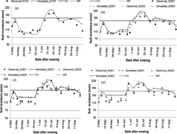
Fig. 1. Observed and simulated soil moisture in the top 0·6 m under various conditions: (a) only rain-fed without supplemental irrigation (SI1) (b) SI2 supplemental irrigation (c) SI3 supplemental irrigation and (d) SI4 supplemental irrigation.

Fig. 2. Observed and simulated canopy cover under various conditions: (a) only rain-fed without irrigation (SI1) (b) SI2 supplemental irrigation (c) SI3 supplemental irrigation and (d) SI4 supplemental irrigation.
Similarly, the simulated CC correlated well with the observed data. There was not much difference between the simulated and observed CC (Fig. 2). All statistical parameters (RMSE, NRMSE and % deviation) showed good results for simulation of soil moisture and CC (data not shown).
The simulated grain yields and total biomass of maize agreed well with that of the observed values under all treatments (Table 5). The NRMSE was between 2 and 7% for grain yield and between 1 and 3% for total above-ground biomass, both of which indicate excellent performance of the model. Similarly, the percentage deviation of the simulated values from the observed values also indicated good agreement.
Table 5. Mean observed and simulated maize grain yield and total biomass with the root mean square error (RMSE), normalized root mean square error (NRMSE) and percentage deviation (Dev.)

SI, supplemental irrigation.
Change in rainfall and temperature
Under ECHAM5 model, the Belg rainfall is projected to decline under both emission scenarios (A2 and B1), while the total rainfall during the Kiremt season is likely to increase under both climate change scenarios (Table 6). Under an ensemble mean of six GCMs, the results of Belg and Kiremt rainfall showed a slight increase under both climate change scenarios, except for a slight decrease during Belg under B1 emission scenarios (Table 6).
Table 6. Percentage change in mean rainfall during Belg and Kiremt seasons for the near future time period using ECHAM5 and ensemble mean of six Global Climate Models (GCMs) under A2 and B1 SRES scenarios against baseline, Halaba, Central Rift Valley, Ethiopia

The projected temperature followed a similar trend, where the highest simulated temperature was during Belg and the lowest was in Kiremt (Table 7). Under both ECHAM5 and ensemble mean of models, the average maximum and minimum temperatures during Belg are likely to increase by 0·9–3·2 °C and 1·0–1·9 °C, respectively. Thus, the Belg season temperature is projected to increase between 1·0 and 3·2 °C in 2050s. During Kiremt, the average maximum and minimum temperatures are likely to increase by 1·0–2·7 °C and 1·6–2·0 °C, resulting in mean Kiremt seasonal temperature changes of 1·0–2·0 °C in 2050s. Both ECHAM5 and Ensemble mean of models showed consistently increasing temperatures in both seasons and annually under the two emission scenarios (A2 and B1) (Table 7). However, the ECHAM5 model projected much larger increases in maximum temperature.
Table 7. Change in maximum and minimum temperature (°C) during Belg and Kiremt seasons and annually for the future time period using ECHAM5 and ensemble mean of six Global Climate Models (GCMs) under A2 and B1 SRES scenarios against baseline period, Halaba, Central Rift Valley, Ethiopia

The supplemental irrigation and plant density level with maximum yield
Based on the 30-year simulation, the irrigation level SI2 (75% TAW depleted) is a better option in terms of increasing grain and total biomass yield and water productivity (Table 8). It was considered a better option because (i) there is a significant difference (P < 0·05) in yield and water productivity between rain-fed (SI1) and the second irrigation level (SI2), (ii) there were no significant further increases in yield and water productivity with higher irrigation levels (SI3 and SI4), (iii) SI2 was enough to save the crop in drought years (when there would have been a total crop failure under rain-fed conditions) and (iv) SI2 requires less irrigation water as compared with the higher levels of supplemental irrigation (SI3 and SI4).
Table 8. Means of grain yield, total biomass and grain water productivity at different levels of supplemental irrigation (SI) and plant density

* Each SI and density level was run for 30 years, d.f. = 29.
Based on the plant density level, yield and water productivity results, the lowest plant density level (D1) was significantly different (P < 0·05) from those achieved with D3 and D4 but not significantly different from the second level plant density (D2) (Table 8). The density levels D2, D3 and D4 also showed no significant difference. However, since yield showed a continuous yield increase as plant density increased from D1 through D4, though some not significant, higher plant density is recommended (75 000 plants/ha) for farmers.
The combined effect of SI and plant density on maize yield shown in Table 9 indicates that yield was not significantly different when the irrigation level was increased beyond SI2. Therefore, the combination of SI2 with plant density D1 (SI2D1), which is significantly different (P < 0·05) from the rain-fed grain and total biomass yield (SI1D1), was used for the subsequent baseline and future yield simulations. Since the density level under rain-fed (SI1D1) and supplemental irrigation (SI2D1) are the same, the yield difference could arise from the supplemental irrigation. Thus, SI2D1 combination hereafter is simply called supplemental irrigation and abbreviated as SI.
Table 9. Means of grain yield and total biomass at different combinations of irrigation and plant density under baseline climate

* Each supplemental irrigation (SI) and density level was run for 30 years, d.f. = 29.
Effect of supplemental irrigation in drought years
Under the baseline climate, SI increased maize grain yield by 20% (yield increased from 6·03 t/ha without SI to 7·26 t/ha with SI) (Fig. 4). This increase in grain yield is in comparison with the 30-year average, which does not clearly show the effect of SI in each year, specifically in drought years. Thus, the response to SI in drought years during the baseline climate was assessed separately, as shown in Table 10.
Table 10. The maximum dry spell (days) and corresponding maize grain yield (t/ha) during drought years and wet year under rain-fed and supplemental irrigation (SI) conditions and total crop water required, available rainfall water and SI used during the first 90 days after sowing (DAS)

1973 was a year with the maximum yield simulated under rain-fed conditions.
From 30 years of baseline climate simulations under rain-fed conditions, the years 1967 and 1972 resulted in total crop failure due to severe drought related to long dry spells during the critical growth stages. The 1967 crop failure was due to a dry spell of >30 days in the period 60–90 days after sowing (DAS), while in 1972 it was due to a dry spell of >20 days that occurred in the 30–60 and 60–90 DAS periods. The crop water requirement for those years was higher than the amount of rainfall, leading to total crop failure. For instance, in 1967, during the first 90 DAS, the crop water requirement (424 mm) was more than twice the available rainfall (188 mm) (Table 10). Simulation results using SI during those severe drought years increased the maize grain yield from total crop failure to 6·8 t/ha. The amount of SI water used to save the crop from total failure ranges between 94 and 111 mm.
In comparison, the year 1973, which showed the maximum grain yield (8·57 t/ha), only suffered a dry spell of <5 days during the critical growth stage (60–90 DAS) and also had larger amount of rainfall compared with crop water requirement during the first 90 DAS. The yield increase due to SI in this year with already high rain-fed grain yield was marginal (2·5%), with the amount of SI water used also very minimal (1·7 mm).
The years 1971 and 1981, despite having limited dry spells (⩽10 days) during the first 90 DAS, still showed very low grain yield as compared with the grain yield in 1973. The very low maize grain yield during these years was due to very high crop water requirement and low amounts of rainfall during the first 90 DAS (Table 10). During 1981, a dry spell of 39 days at 90–120 DAS contributed to the low grain yield but not to the extent of total crop failure. The use of SI would have increased grain yields by 59–62% for those years with very low rain-fed grain yield (1971 and 1981).
The sowing date/onset for the years simulated with crop failure (1967 and 1972) and very low grain yield (1971 and 1981) were during the month of March or early April, whereas the sowing date/onset for the year with maximum yield (1973) was in the month of May.
Effect of climate change on dry spells
The projected percentage change in the longest mean dry spell in each month of the Belg and Kiremt seasons for the future climate (2020–49) compared with the baseline climate (1966–95) is shown in Table 11.
Table 11. Percentage change (%) in the longest dry spell for March–October for future climate under ECHAM5 and ensemble mean of models on A2 and B1 SRES scenarios against the baseline longest dry spell (days)

The first three months (March–May) are the Belg (short rainy season) while the 5 months (June–October) are the Kiremt (main rainy season). The Kiremt season is usually considered to be June–September but sometimes it can be extended to include October.
Under the baseline climate, all months of the Belg season showed the longest mean dry spell as being between 12 and 15 days. During the Kiremt season, particularly in July, August and September, the longest mean dry spells were <10 days. October, which is usually considered to be out of the Kiremt season, had a longest mean dry spell of 22 days. The month of October was included because in some years, when the sowing of maize goes as late as the first week of July, a 120–150 DAS growing period can extend into October. Thus, rainfall conditions during October can sometimes affect yield.
Under the ECHAM5 model, the projected length of dry spells for March and April increased by 20–25% and 4–5% under A2 (high) and B1 (low) emission scenarios, respectively. By contrast, the projected longest dry spell between June and October decreased by 7–42% and 6–55% under A2 and B1 scenarios, respectively, except in August where there was almost no change under the B1 scenario. The projected longest dry spells under the A2 scenario was always higher than under B1 scenario.
Under ensemble mean of models, the projected longest dry spell decreased for almost all months except March and May, where there was a modest increase under both scenarios. With both models and scenarios, the decrease in projected longest dry spell was greatest for October.
Effect of carbon dioxide level on maize yield
With the ECHAM5 model, the simulated maize grain yield under projected climate change scenarios using the reference CO2 level (369·14 ppm) showed decreases of 22 and 9% under A2 and B1, scenarios, respectively, compared with the baseline climate simulation (Fig. 3). Under ECHAM5 model, both rainfall analysis (Table 6) and dry spell analysis (Table 11) consistently showed a drying Belg (March–April), despite Kiremt getting wetter. Since maize is sensitive to moisture stress during the first 30 DAS and between 60 and 90 DAS, later stages of maize are less sensitive to moisture stress. Therefore, since most sensitive stages are during Belg, assuming early Belg sowing, maize yield is more affected during Belg season dry spells. That could be the reason behind the decline in maize yield under ECHAM5 projection as compared with baseline yield.

Fig. 3. Baseline and Projected (proj.) maize grain yield under reference (ref.) CO2 (369·14 ppm) and projected CO2 level on ECHAM5 and ensemble mean model under high (A2) and low (B1) emission scenarios in Halaba special Woreda, Central Rift Valley, Ethiopia. Error bars indicate the 95% confidence interval of the mean.
Using the ensemble mean of models, the simulated maize grain yield under the same conditions decreased slightly (6%) under the A2 scenarios, whereas it stayed almost the same for the B1 scenario compared with the baseline climate simulation (Fig. 3).
With elevated CO2 concentrations, under projected climate variables, grain yield increased compared with the simulations using reference CO2 with both GCM models. Under ECHAM5, the simulated grain yield increased by 7·5% when CO2 concentration level increased from the reference 369·41–518·88 ppm under the A2 scenario, and by 6·2% when CO2 concentration level increased from the reference 369·41–467·57 ppm under the B1 scenario. Under similar CO2 increases, for the ensemble mean of models, the yield increased by 7·4 and 6·4% under A2 and B1 scenarios, respectively (Fig. 3).
Effect of supplemental irrigation on maize yield
Figure 4 presents maize grain yield under rain-fed and SI conditions for different climate change scenarios. The ECHAM5 model, with the A2 scenario and SI, showed an increase in grain yield of 8% against the baseline yield, and of 38% against the projected rain-fed grain yield. Similarly, with the B1 scenario, SI increased the grain yield by 8% against baseline yield and by 19% against the projected rain-fed grain yield.

Fig. 4. Maize grain yield (t/ha) under rain-fed and supplemental irrigation (SI) for baseline and future climate conditions. The blue bold lines indicate the mean deviation. Boxes indicate inter-quartile ranges and error bars indicate minimum and maximum values.
Under the ensemble mean of models with the A2 scenario, SI increased the grain yield by 15% against the baseline yield and by 13% against the projected rain-fed grain yield. The ensemble mean of models with the B1 scenario and SI showed an increase in grain yield of 19% against baseline yield and of 11% against projected rain-fed grain yield. On both ECHAM5 and ensemble mean of models, when the projected grain yield was compared between rain-fed and SI conditions, the effect of SI for the A2 scenario was higher than for the B1 scenario.
Effect on maize yield of shifting the sowing date
Table 12 presents the percentage change in grain yield when the sowing dates are in April, May and June compared with the baseline sowing date of April. Using the ECHAM5 model with the A2 scenario, the simulated grain yield decreased by 61 and 2% when sowing date was in April and May, respectively, but an increase of 96% when sowing date was delayed until June. The ECHAM5 model with the B1 scenario simulated a grain yield decrease of 37% when sowing of maize was in April but an increase of 35% when sowing was in May. When the sowing of maize was further extended to June, the grain yield increased by 140% under the B1 scenario.
Table 12. Percentage change (%) in projected maize grain yield in different sowing months respective to baseline yield under ECHAM5 and ensemble mean models with A2 and B1 SRES scenarios
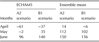
Under the ensemble mean of models, sowing of maize in any of the months will increase yield under both A2 and B1 scenarios except in April, where maize grain yield decreased slightly under the B1 scenario. Overall, maximum yield was obtained when the sowing of maize was extended to June under both models and scenarios.
DISCUSSION
The aim of the current study was (i) to determine the best combination of SI and plant density using 30 years of baseline climate, to be used in future climate scenarios, (ii) to assess drought for the baseline and future climate using dry spell analysis and (iii) to evaluate the adaptation options of SI, plant density and shifting of the planting date for improving maize grain yield and improved food security.
AquaCrop validation
A key part of achieving the aims of the current study was validation of the AquaCrop model. AquaCrop has proven to show good performance in simulating soil moisture, CC, grain yield and total biomass under different levels of irrigation treatments elsewhere (Abedinpour et al. Reference Abedinpour, Sarangi, Rajput, Man, Pathak and Ahmad2012, Reference Abedinpour, Sarangi, Rajput and Man2014). Similarly, AquaCrop has also been validated for maize elsewhere in Ethiopia and reported that it can simulate grain yield and total biomass well (Erkossa et al. Reference Erkossa, Awulachew and Aster2011; Biazin & Stroosnijder Reference Biazin and Stroosnijder2012). Therefore, due to its simplicity, accuracy and robustness, AquaCrop is becoming a widely used model for estimating crop yield for climate change scenarios and to test different adaptation options (Mainuddin et al. Reference Mainuddin, Kirby and Hoanh2011, Reference Mainuddin, Kirby and Hoanh2013; Soddu et al. Reference Soddu, Deidda, Marrocu, Meloni, Paniconi, Ludwig, Sodde, Mascaro and Perra2013; Abedinpour et al. Reference Abedinpour, Sarangi, Rajput and Man2014; Shrestha et al. Reference Shrestha, Thin and Deb2014, Reference Shrestha, Deb and Bui2016; Vanuytrecht et al. Reference Vanuytrecht, Raes, Willems and Semenov2014; Deb et al. Reference Deb, Shrestha and Babel2015; Muluneh et al. Reference Muluneh, Biazin, Stroosnijder, Bewket and Keesstra2015). The AquaCrop model was able to simulate the soil water, CC and crop yields well for the BH540 maize cultivar under both rain-fed conditions and different levels of SI with conservative and user specific crop parameters. The values of RMSE, NRMSE and percentage deviation for the model validation were all in acceptable ranges.
Change in rainfall and temperature
The change in rainfall for future climate in Halaba district is almost consistent with previous results found in the CRV, with rainfall during the Belg and Kiremt seasons decreasing and increasing, respectively (Muluneh et al. Reference Muluneh, Biazin, Stroosnijder, Bewket and Keesstra2015). Therefore, the projected decrease in Belg rainfall will negatively affect long-cycle crop yields (e.g. maize) in the CRV.
The projected temperature increase generally agrees with other studies in Ethiopia and elsewhere. For example, Admassu et al. (Reference Admassu, Getinet, Thomas, Waithaka and Kyotalimye2012) reported a temperature increase of 1·5–2 °C in 2050 in some areas of Ethiopia using the Model for Interdisciplinary Research on Climate (MIROC) and Commonwealth Scientific and Industrial Research Organisation (CSIRO) GCM models. Similarly, Conway & Schipper (Reference Conway and Schipper2011) reported a temperature increase of 1·4–2·9 °C in 2050s in most regions of Ethiopia using 18 GCM averages. Many GCMs project mean average temperature increases to 2050 for the East Africa region larger than the global mean: for example, for scenario A2, increases of between 1·5 and 2·5 °C have been projected (Jones & Thornton Reference Jones and Thornton2013).
Yields will be reduced when the optimal temperature ranges of crops are exceeded (Adams et al. Reference Adams, Hurd, Lenhart and Leary1998; Wheeler et al. Reference Wheeler, Craufurd, Ellis, Porter and Prasad2000). The optimal temperature range for C4 summer crops such as maize was set by Hsiao et al. (Reference Hsiao, Heng, Steduto, Rojas-Lara, Raes and Fereres2009) as 8–30 °C. Similarly, Lobell et al. (Reference Lobell, Bänziger, Magorokosho and Vivek2011) found statistically insignificant effects of temperature on maize yields to increased degree days between 8 and 30 °C. The same study (ibid) also found that maize yields in Africa may gain from warming at relatively cool sites (such as Ethiopia, where average growing-season temperatures in most regions are <30 °C), but are significantly reduced in areas where temperatures commonly exceed 30 °C. This was clearly observed in the current work, in temperature analysis for baseline and projected scenarios; despite showing increased projected temperature, it remains in the range where there is no significant effect on the maize crop (between 8 and 30 °C). Generally, these temperature ranges fall inside the temperature regimes favouring the growth and production of maize. Other studies also indicated towards this trend, where although crop yield could be affected by both precipitation and temperature, it is more sensitive to the precipitation than temperature (Akpalu et al. Reference Akpalu, Hassan and Ringler2008; Kang et al. Reference Kang, Khan and Ma2009). However, any temperature increase will increase rates of evapotranspiration, possibly leading to a deficit in the water balance and posing a major challenge to rain-fed agriculture.
The supplemental irrigation and plant density level with maximum yield
After simulating yield with ten different combinations of SI and plant density for each year of the 30-year baseline period, the means of simulated yield were compared to determine the best combination of SI and plant density. Among the ten combinations of SI and plant density, SI2D1 (i.e., application of SI when the SWD of the TAW reached 75% using 30 000 plants/ha) simulated maximum grain yield and total biomass. The maize crop density level most commonly used by farmers in the CRV is 30 000–40 0000 plants/ha. Despite a continuous grain yield increase from lower SI and plant density combination to higher level combination, the difference was not statistically significant. Therefore, the combination with the lowest SI level was chosen (S2D1).
Effect of supplemental irrigation in drought years
The 30-year mean yield increase from SI was modest. However, this long-term mean yield cannot show how the crop responds to SI in a particular drought year when there would be total crop failure under rain-fed conditions. Therefore, the effect of SI was analysed on crop yield under conditions where there would be total rain-fed crop failure or very low crop yield. Total crop failure during drought years was due to a dry spell of >30 days during the 60–90 DAS period (1967) and dry spells of >20 days in both the 30–60 and 60–90 DAS periods (1972). Another study in the semi-arid part of the CRV by Biazin & Sterk (Reference Biazin and Sterk2013) found that dry spells longer than 30 days occurring in the first 60 DAS, or longer than 20 days in the 60–90 DAS period, were critical and caused total crop failure for maize crops. This confirms that the most damaging effect of dry spells is manifested during sensitive stages of crops such as flowering and grain filling, which has also been documented by Stern & Coe (Reference Stern and Coe1984).
The current analysis showed that by using 94–111 mm of SI during sensitive stages of maize crop, it is possible to avoid total crop failure. Similarly, Magombeyi et al. (Reference Magombeyi, Rasiuba, Taigbenu, Humphreys and Bayot2009) in South Africa found that using 110 mm of SI in the driest year of their research resulted in the highest yield responses. The availability of water for SI is an important factor for evaluating and determining effective SI strategies, as determined in another similar study in the CRV (Muluneh et al. unpublished). The results of that research showed that sufficient amounts of water for SI would be available from existing farm ponds, even in drought years.
Effect of climate change on dry spells
With respect to predicting the length of dry spells, the two climate models used showed consistent results. Both models indicate increasing tendency of dry spells during Belg (March and April) and a decreasing tendency during Kiremt (June-October). However, during Belg the ECHAM5 model showed more dryness than the ensemble mean of models. Most other studies also indicate the drying tendency of the Belg season, mostly in the Ethiopian highlands. For example, recently, Cook & Vizy (Reference Cook and Vizy2012) using ten GCM ensemble mean models found that the number of dry days in the Ethiopian Highlands is likely to increase by 5–20 days, a 2–10% increase during 2041–60 compared with 1981–2000. This future increase in dryness was associated with a reduction of the Belg (March–May) rainfall.
The drying of Belg is consistent with the declining March–June rainfall that occurred during the second half of the 20th century and which is projected to continue into the future in the East African region, particularly in Ethiopia (Funk et al. Reference Funk, Dettinger, Michaelsen, Verdin, Brown, Barlow and Hoell2008; Williams & Funk Reference Williams and Funk2011; Lyon & DeWitt Reference Lyon and DeWitt2012; Muluneh et al. Reference Muluneh, Biazin, Stroosnijder, Bewket and Keesstra2015). Agricultural production in the Ethiopian CRV takes place in two cropping seasons per year, the Kiremt and Belg seasons. Belg rains are critical for long-cycle crops (such as maize and sorghum), which are harvested at the end of the Kiremt season. Belg-dependent growing areas are typically the most food-insecure cropping areas (World Food Programme 2014). Therefore, the predicted effects of Belg season drought could exacerbate future livelihood degradation and food insecurity in the CRV of Ethiopia.
Furthermore, the two climate models used are consistent in showing the cessation of rainfall in the future likely to be extended compared with the current climate. This may extend the growing season into October, which could allow a later sowing date (see later). This could compensate, at least in part, for the predicted increase in dry spells during Belg drought.
Effect of carbon dioxide level on maize yield
With both ECHAM5 and the ensemble mean of models, the projected maize grain yield showed a declining tendency in the dry sub-humid area of the CRV. On the other hand, when both GCM models were run with elevated CO2 concentrations, they showed increasing grain yields. Similarly, Muluneh et al. (Reference Muluneh, Biazin, Stroosnijder, Bewket and Keesstra2015) reported maize grain yield increases from elevated CO2 in the CRV.
Generally, there is a consensus that elevated CO2 tends to increase growth and yield of most agricultural plants as a result of higher rates of photosynthesis and low rates of water loss that improve water-use efficiency (Allen & Amthor Reference Allen, Amthor, Woodwell and Mackenzie1995; Parry et al. Reference Parry, Rosenzweig, Iglesias, Livermore and Fischer2004; Vanuytrecht et al. Reference Vanuytrecht, Raes and Willems2011). However, the question is, can the yield increase from elevated CO2 fully compensate the yield decline caused by climate change? In the current study, the ensemble mean of models yield projection elevated CO2 level was able to offset the negative impact of climate change, because there was not too much difference between the projected simulated yield and the baseline simulated yield. However, the ECHAM5 model projection, despite the 7·5% yield increase from elevated CO2 level, still shows grain yield to be less than the baseline climate simulation, because the projected simulated yield was much lower than the baseline simulated yield. Thus, despite the positive effect of elevated CO2 to crops, the predicted lower maize production due to the changing rainfall is only partly compensated by the expected increase in CO2 concentration.
Effect of supplemental irrigation on maize yield
The simulated maize yield using SI for future climate scenarios proved that SI can offset the predicted yield reduction due to climate change. With SI, the 22% simulated yield reduction from the ECHAM5 model for the A2 scenario and rain-fed climate becomes an 8% increase. The ensemble mean of models projected a similar increase in simulated yield under SI. Thus, SI is a promising adaptation option for farmers in the CRV. Although, due to the expected increase in dry spells, sowing of maize under rain-fed conditions during Belg is becoming riskier, SI is a strategy to enable growing of long-maturing maize varieties that can still be sown during the Belg season.
Effect of shifting the sowing date
The average sowing date for the baseline climate is in April. If the baseline sowing date is used for future climate scenarios, the yield is affected negatively unless additional measures are taken. However, from the results of both ECHAM5 and ensemble mean of models, shifting sowing of maize from April to June (from mid-Belg to the start of Kiremt) for future climate conditions increases the maize grain yield. These results are consistent with research findings elsewhere in Africa. In Ghana, Tachie-Obeng et al. (Reference Tachie-Obeng, Akponikpè and Adiku2013) reported that delaying sowing dates by 6 weeks, from the baseline date of 1 May to 15 June, increased maize yields by up to 12%. For projected future climate conditions, the sowing of maize in June will decrease the risk of crop failure, since dry spells continuously decrease from June to October.
Furthermore, the projected decrease in the longest dry spell as the Kiremt months progress (June–October) indicates an extension to the end of Kiremt rainfall, thus increasing the length of the crop growing period. This is consistent with a previous study that reported the lengthening of the growing season in the CRV of Ethiopia due to the later cessation of Kiremt (Muluneh et al. Reference Muluneh, Biazin, Stroosnijder, Bewket and Keesstra2015). Other studies also indicated that the simulated annual cycle for Ethiopia shows a shift in both the rainfall onset and cessation dates, by about a month (Shongwe et al. Reference Shongwe, van Oldenborgh, de Boer, van den Hurk and van Aalst2008). This result implies a shift in the whole rainy season, with October receiving more rainfall than in the present climate.
Generally, in the Ethiopian highlands, climate change may extend the agricultural growing seasons as a result of increased temperatures and rainfall changes (Thornton et al. Reference Thornton, Jones, Owiyo, Kruska, Herrero, Kristjanson, Notenbaert, Bekele and Omolo2006; Boko et al. Reference Boko, Niang, Nyong, Vogel, Githeko, Medany, Osman-Elasha, Tabo, Yanda, Parry, Canziani, Palutikof, van der Linden and Hanson2007). According to Segele & Lamb (Reference Segele and Lamb2003), warm sea surface temperatures in the Indian Ocean and Arabian Sea are likely to be associated with delayed Kiremt cessation and hence prolonged rain. Therefore, shifting the sowing period of maize from the baseline Belg season (mostly April or May) to the first month of Kiremt season (June) seems to be a promising adaptation to increase food security in the face of expected climate change.
CONCLUSIONS
A change in climate in the CRV of Ethiopia is inevitable and maize yield will decline if no changes in cropping practices are made to adapt to the future climatic conditions (2020–49). In the current study, the projected changes in dry spells, rainfall, CO2 levels and their effect on maize grain yield were assessed in dry sub-humid and semi-arid parts of the Ethiopian CRV. Then a validated crop simulation model was used to explore three adaptation options: plant density, SI and shifting of the sowing date. From the results of the assessment and analysis reported above, the following conclusions have been drawn regarding the adaptation options:
-
1. Increasing plant density from 30 000 to 75 000 plants/ha showed statistically significant yield increase. So, higher plant density is recommended (75 000 plants/ha).
-
2. Supplemental irrigation is a promising option for crop survival and improving yield and therefore food security. Although SI has a marginal effect in good rainfall years, using 94–111 mm of SI during sensitive growth stages can avoid total crop failure in drought years. From earlier research conducted in the area it was proved that this amount of SI can be available using farm ponds catching runoff, even in drought years (Muluneh et al. unpublished).
-
3. Shifting the sowing period of maize from the current Belg season (mostly April or May) to the first month of Kiremt season (June) is another promising adaptation for increasing food security in the face of expected climate change. The climate models used predicted a temporal shift in rainfall, meaning even less in Belg and more in Kiremt, thus extending the growing season. Shifting the sowing period can reduce the risk of crop failure and offset the predicted yield reduction caused by climate change.
The authors express their sincere appreciations to the Netherlands Organization for International Cooperation in Higher Education (NUFFIC) and International Foundation for Science (IFS) for supporting the research financially. The authors are thankful to the farmers who generously made their farm fields and water stored through water harvesting ponds available for field experimentations. The authors are also thankful to Demie Moore for her language editorial support.


