


1. INTRODUCTION
Ice shelves control the drainage of grounded ice into the ocean fringing two-thirds of Antarctica (Bindschadler and others, Reference Bindschadler2011). Through lateral friction from the embayment sides or local pinning points that create a backstress (Matsuoka and others, Reference Matsuoka2015; Berger and others, Reference Berger, Favier, Drews, Derwael and Pattyn2016), they buttress glaciers and ice streams (Dupont and Alley, Reference Dupont and Alley2005; Gudmundsson, Reference Gudmundsson2013). Upon their sudden disintegration, glaciers that originally fed the ice shelves have been observed to speed up (De Angelis and Skvarca, Reference De Angelis and Skvarca2003; Scambos and others, Reference Scambos, Bohlander, Shuman and Skvarca2004), accelerating the transfer of land ice into the ocean where it eventually melts and contributes sea level rise. It is thus important to understand what controls the stability of ice shelves.
Generally, thinning ice shelves are less stable than thickening ice shelves. A potentially long-lived ice-shelf accretes new mass not only through dynamic inflow from glaciers and ice streams but also through local accumulation of snow on the ice-shelf surface (Depoorter and others, Reference Depoorter2013; Rignot and others, Reference Rignot, Jacobs, Mouginot and Scheuchl2013a) and through basal freezing on (Fricker and others, Reference Fricker, Popov, Allison and Young2001; Pritchard and others, Reference Pritchard2012; McGrath and others, Reference McGrath2014; Moholdt and others, Reference Moholdt, Padman and Fricker2014) generating so-called marine ice (Tison and others, Reference Tison, Ronveaux and Lorrain1993). Ice shelves that accrete more basal ice than they lose ice due to melting have been called cold-cavity ice shelves (Rignot and others, Reference Rignot, Jacobs, Mouginot and Scheuchl2013a). Warm-cavity ice shelves primarily melt at their base due to warm ocean currents (Rignot and others, Reference Rignot, Jacobs, Mouginot and Scheuchl2013a), sometimes in distinct basal channels (Vaughan and others, Reference Vaughan2012; Alley and others, Reference Alley, Scambos, Siegfried and Fricker2016) that can be mirrored by surface melting (Dow and others, Reference Dow2018), further thinning the ice-shelf and thus decreasing its stability. As a result of dynamic flow and heterogeneous stucture, ice shelves also develop brittle weaknesses, such as crevasses and rifts (Rack and Rott, Reference Rack and Rott2004; De Rydt and others, Reference De Rydt, Hilmar Gudmundsson, Nagler, Wuite and King2018; King and others, Reference King, De Rydt and Hilmar Gudmundsson2018), resulting in ice mass loss through ice berg calving (Liu and others, Reference Liu2015; Jansen and others, Reference Jansen2015), possibly as a result of hydrofracturing if combined with surface melting (Banwell and Macayeal, Reference Banwell and Macayeal2015). If more than just the passive shelf ice is removed, ice-shelf restraint is decreased (Fürst and others, Reference Fürst2016), also with the possibility of sudden ice-shelf disintegration (Scambos and others, Reference Scambos, Hulbe and Fahnestock2003, Reference Scambos2009; Cook and Vaughan, Reference Cook and Vaughan2010). When ice shelves are heterogeneous and composed partially of marine ice, the propagation of crevasses could be slowed (McGrath and others, Reference McGrath2014) due to the different temperature and material properties of marine ice (Dierckx and Tison, Reference Dierckx and Tison2013).
Understanding the surface and basal boundary conditions of ice shelves can help in assessing ice-shelf mass balance and stability. Most previous studies use a combination of altimetry remote sensing products or airborne radar data to derive the ice-shelf surface elevation or meteoric ice thickness, respectively, and assume hydrostatic equilibrium to constrain the basal boundary of the ice-shelf (Fricker and others, Reference Fricker, Popov, Allison and Young2001; Depoorter and others, Reference Depoorter2013; Rignot and others, Reference Rignot, Jacobs, Mouginot and Scheuchl2013a; Moholdt and others, Reference Moholdt, Padman and Fricker2014; Liu and others, Reference Liu2015). Additionally, assumptions regarding firn extent and density have to be made (Ligtenberg and others, Reference Ligtenberg, Helsen and van den Broeke2011). Very few studies have actually determined firn density using in situ methods (Medley and others, Reference Medley2013; Kuipers Munneke and others, Reference Kuipers Munneke2017), especially since the density can vary spatially and with depth due to refreezing of surface meltwater (Hubbard and others, Reference Hubbard2016; Bevan and others, Reference Bevan2017). Constraining basal ice-shelf boundary conditions in situ is logistically even more challenging and only few studies have succeeded in excavating ice cores from the basal marine ice (Oerter and others, Reference Oerter1992; Tison and others, Reference Tison, Ronveaux and Lorrain1993; Treverrow and others, Reference Treverrow, Warner, Budd and Craven2010) and rely mostly on a combination of ice penetrating radar data collected on the ground and GPS measurements (Jansen and others, Reference Jansen, Luckman, Kulessa, Holland and King2013; McGrath and others, Reference McGrath2014). Smaller scale basal crevasses can also be detected this way (Arcone and others, Reference Arcone2016).
We use the radar statistical reconnaissance (RSR) technique (Grima and others, Reference Grima, Schroeder, Blankenship and Young2014b) applied to a 2014–15 very-high frequency (VHF) airborne radar survey acquired by the High Capability Radar Sounder 2 (HiCARS2) to assess the distribution of surface density and roughness of the southern McMurdo Ice Shelf (SMIS) and part of the Ross Ice Shelf (RIS). Surface density derived from airborne data replaces in situ efforts of using firn cores in combination with surface height changes from automatic weather station data. It also extends the geographical coverage of accumulation rates derived from isochrone depths that are extracted from ground penetrating radar profiles (Medley and others, Reference Medley2013). Surface roughness is relevant for more sophisticated ablation models using energy balance (van den Broeke and others, Reference van den Broeke, Smeets and Ettema2009) and helpful in detecting zones of large-scale roughness features such as surface melt ponds and former percolation areas (Banwell and Macayeal, Reference Banwell and Macayeal2015; Rutishauser and others, Reference Rutishauser2016; Bevan and others, Reference Bevan2017). We extend the application of RSR to the basal ice reflector of SMIS and RIS. The derived signal characters are related to the basal composition and geometric heterogeneities, both of which are indicators of basal mass balance controlled locally through melting and accumulation of frazil ice crystals during the formation of marine ice (i.e., accretion). This basal roughness has been suggested to be a crucial parameter in the redistribution of the melt/freeze pattern and the alteration of vertical circulation across the ice-shelf and, therefore, its long-term evolution and stability (Gwyther and others, Reference Gwyther, Galton-Fenzi, Dinniman, Roberts and Hunter2015)
We first present the regional context related to the SMIS and RIS and describe the airborne radar data set used. Then, we introduce the RSR technique applied to the surface radar return and detail a new model for the inversion of the basal character from application of the RSR technique to the basal radar return. We present the results for both the surface and the base; subsequently using these characteristics to identify and classify basal units. Interpretations and hypotheses to account for the observed basal units and their radar properties are discussed in terms of basal melting and marine ice accretion and distribution.
2. CONTEXT
2.1. Regional setting
The SMIS is a small ice-shelf in Antarctica adjacent to, but separated from, the much larger RIS by a rift zone. SMIS has a heterogeneous ice composition and is made up of meteoric and marine ice, which is exposed at the surface in its south due to a negative surface ablation (Kellogg and others, Reference Kellogg, Kellogg and Stuiver1991; Fitzsimons and others, Reference Fitzsimons, Mager, Frew, Clifford and Wilson2012a; Koch and others, Reference Koch, Fitzsimons, Samyn and Tison2015). Since there is a large thickness difference to the adjacent RIS, a steep basal gradient to the much thinner SMIS likely facilitates generation of frazil ice crystals from buoyant supercooled melt water and thus the formation of basal marine ice (Koch, Reference Koch2016). Due to its large surface gradients in local accumulation (Clifford, Reference Clifford2005; Koch, Reference Koch2016), SMIS is believed to sustain itself.
The RIS is nourished by the inflow of prominent ice streams from the East and West Antarctic Ice Sheets (Rignot and others, Reference Rignot, Mouginot and Scheuchl2011), but has shown little overall thickness changes in recent years (Pritchard and others, Reference Pritchard2012). RIS is a cold-cavity ice-shelf (Rignot and others, Reference Rignot, Mouginot, Larsen, Gim and Kirchner2013b), but experiences some basal melting to its west (Dinniman and others, Reference Dinniman, Klinck and Smith2007). A thin layer of marine ice has been detected at the base of the center of the ice-shelf (Zotikov and others, Reference Zotikov, Zagorodnov and Raikovsky1980), the small basal accumulation is likely ascribed to its shallow basal gradient (Depoorter and others, Reference Depoorter2013) that does not promote fast supercooling of basal meltwater and thus the fast generation of frazil ice crystals (Martin, Reference Martin1981; Daly, Reference Daly1984) that agglomerate to form marine ice (Treverrow and others, Reference Treverrow, Warner, Budd and Craven2010).
2.2. Data
HiCARS2 is a 60-MHz central frequency (f), 5-m wavelength (λ), 15-MHz bandwidth (B), airborne radar sounder maintained and operated by the University of Texas, Institute for Geophysics (UTIG) and flown on board a Basler BT-67. This radar system is similar to HiCARS (Peters, Reference Peters2005) with upgraded components (Grima and others, Reference Grima2016). The surface area illuminated by HiCARS2 is 200–400 m in diameter (pulse-limited footprint), growing with the aircraft range to the surface. Pulse compression by matched filtering provides a range (i.e., vertical) resolution $\delta v = c/(2B\sqrt {\epsilon })$ , where c is the speed of light in vacuum and ε the dielectric constant (permittivity) of the sounded material, ranges from ~5.6 m in pure ice (ε = 3.15) to ~ 9.5 m in dry-snow (ε = 1.1) (Kovacs and others, Reference Kovacs, Gow and Morey1995).
The studied HiCARS2 data set was acquired during the 2014–15 austral summer and covers most of the SMIS extent and part of the RIS lying south of Minna Bluff (Fig. 1). Although the survey covers the northern McMurdo Ice Shelf (MIS), this region has not been studied since a brine layer in the firn prevents the detection of the ice/ocean interface at this wavelength and over a significant portion of the ice-shelf (Grima and others, Reference Grima2016). We have calibrated the signal from the surface return over the blue-ice outcrop in MIS depicted by Grima and others (Reference Grima2016) in their Figure 1, and assuming a permittivity of 3.15 for the surface.
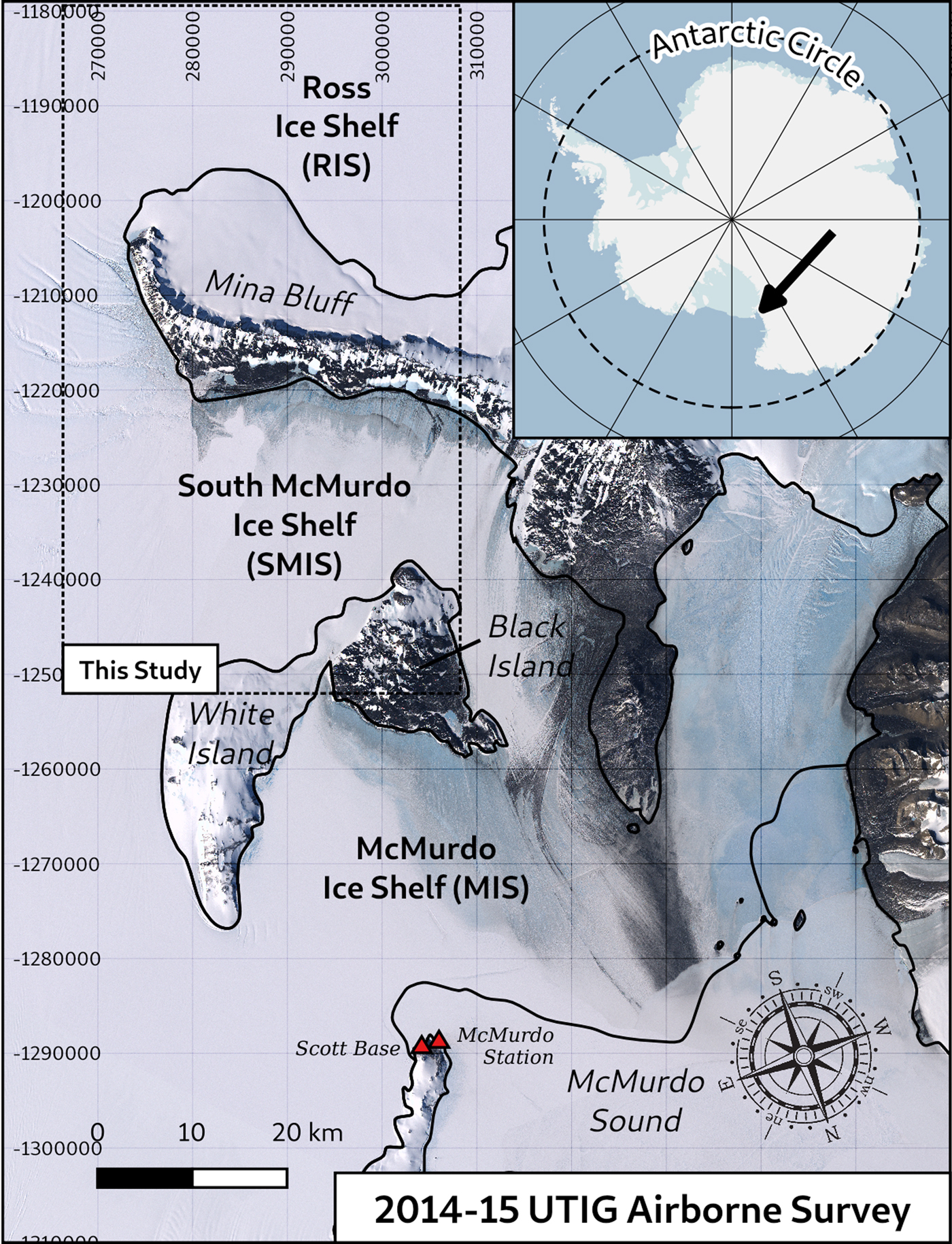
Fig. 1. Continental and regional maps illustrating the geographic context of the southern McMurdo Ice Shelf overlaid by the 2014–2015 UTIG airborne survey tracks (red lines). This study addresses the portion of the tracks covering SMIS and RIS. The background is the Landsat image mosaic of Antarctica (Bindschadler and others, Reference Bindschadler2008). All the maps in this manuscript use a standard universal polar stereographic (UPS) projection with a metric-based cartesian ‘easting/northing’ coordinate system.
The radar signal is reflected/scattered back to the antenna by every dielectric gradient on its propagation path until signal extinction. As the signal is transmitted at high repetition frequency along-track (~2000 Hz for HiCARS2), a vertical cross-section is built providing subsurface dielectric horizons with a time-delay vertical axis. The surface-subsurface echo time-delay (t) is related to depth (h) through the velocity of light in the medium (c) by $t=2h\sqrt {\epsilon }/c$ . We have inverted h for the first echo below the surface (when present) by considering ε = 3.1 (i.e., pure meteoric ice). The RSR technique, explained in more details in Section 3, is a radiometric approach essentially using the strength of a given echo as an observable.
3. METHOD
3.1. Principles
The energy radiated back to the antenna from a dielectric interface (e.g., air–ice or ice–ocean) is the coherent summation of all elementary electric fields reflected and scattered by the dielectric contrasts within a volume bounded horizontally by the circular radar footprint and vertically by the radar range resolution. Therefore, the echo strength holds crucial information about the composition and macro-structure (>1% the wavelength in size) near the considered interface (Grima and others, Reference Grima, Schroeder, Blankenship and Young2014b). The RSR technique aims to provide two parameters to further characterize the echo strength and the properties of the related interface: (1) coherent energy reflected by the regularly distributed dielectric gradients, and (2) incoherent energy scattered by the random discontinuities of the medium. It can be shown analytically that the total energy received is the summation of both the coherent and incoherent ones (Ulaby and others, Reference Ulaby, Moore and Fung1981).
The RSR technique has been applied to the surface echo over a wide range of planetary ice masses using airborne radar data: The Thwaites Glacier catchment and the northern MIS in Antarctica (Grima and others, Reference Grima, Blankenship, Young and Schroeder2014a,Reference Grima, Schroeder, Blankenship and Youngb, Reference Grima2016) and the Devon Ice Cap in the Canadian Arctic (Rutishauser and others, Reference Rutishauser2016) for characterization of the firn density, surface roughness, near-surface brine, and refrozen ice from downward percolation. Using satellite radar data, the RSR surface technique has also successfully been applied on Mars for supporting the landing site selection of the NASA's InSight lander (Putzig and others, Reference Putzig2017) and to measure the waves riddling the hydrocarbon seas of Saturn's largest moon Titan (Grima and others, Reference Grima2017).
Derivation of both coherent and incoherent energies are obtained by best-fitting the amplitude distribution of a set of surface echoes with a theoretical stochastic envelope whose parameters are a function of the coherent and incoherent energies (Destrempes and Cloutier, Reference Destrempes and Cloutier2010). We use an envelope derived from Homodyne K-statistics (HK), a flexible model that does not require the condition of large scatterer numbers to be fulfilled and allows the scatterers to be clustered (non-stationarity) within the radar footprint (Jakeman, Reference Jakeman1980; Jakeman and Tough, Reference Jakeman and Tough1987). Here, we apply the RSR in the same manner as Grima and others (Reference Grima2016), i.e., the along-track data are divided into 1-km sampled spaces (~1000 surface echoes each) repeated every 250 m. A set of signal component pairs is then derived for every sampled space for both the surface echo and the first subsurface echo (when present) occurring after the surface return. In the following, the first subsurface return is called basal echo and is considered to be the base of the meteoric ice.
3.2. Forward model
Here we present a forward model to bound the received coherent–incoherent energy pairs to their respective coefficients describing the surface and basal reradiation properties. We consider a three-layer model where the horizontal medium 1 (ice) of thickness h 1 is sandwiched between the two half-spaces 0 (air) and 2 (ocean), respectively. The antenna lies in medium 0 and transmits down a coherent source of power P 0 at a distance h 0 from the surface bounded by 0 and 1. The energy radiated back by the surface and the basal interface (bounded by 1 and 2) and intercepted by the antenna is P s and P b, respectively, such as


where the diacritic dot and tilde indicate the coherent and incoherent components of the signal, respectively. The link budget is the relationship between the energy transmitted by the source and the energy received at the antenna. It describes the propagation history of the signal and depends on the interface coefficients describing its capability to reradiate the energy of an impinging signal. For a rough surface in the normal direction, the interface coefficients are the effective reflectance (${\dot R}$ ) and transmittance (${\dot T}$
 ) for the coherent part of the signal, as well as the backscatter (${\tilde R}$
 ) and forward-scatter ($\tilde {T}$
 ) coefficients for the incoherent part. The expressions for both ${\dot P}_{\rm s}$
 and $\tilde {P_{\rm s}}$
 can be derived from their link budget, considering the surface as a specular reflector and as a scattering center, respectively:

where α is a calibration factor in square meters accounting for the instrumental gains and including the antenna aperture. L(z) = 1/(4πz 2) are the losses from isotropic geometric spreading along a distance z, and A s is the footprint area at the surface. Likewise, the link budget for ${\dot P}_{\rm b}$ and $\tilde {P_{\rm b}}$
 can be obtained from their propagation history illustrated by Figure 2. At each interface, the impinging signal is broken out into a coherent and incoherent signal modulated by the interface coefficients, and so on, so that P b is the sum of eight contributions, $P_{{\rm b}_1}$
 to $P_{{\rm b}_8}$
 , each with their own propagation history.


where Q 1 is the one-way attenuation in medium 1, the s and b subscripts denote the surface and basal coefficients, respectively, while A b is the pulse-limited footprint area at the basal interface. Of interest, we note symmetries in propagation histories so that $P_{{\rm b}_2}=P_{{\rm b}_5}$ and $P_{{\rm b}_4}=P_{{\rm b}_7}$
 . Among those contributions, only $P_{{\rm b}_1}$
 keeps a coherent character since it is not affected by a scattering coefficient. Hence, the coherent and incoherent powers detected at the antenna can be written as


It is worth noting that the above model allows a portion of the incoming coherent energy to be transferred into incoherent energy at each reflection/transmission. Conversely, it does not allow for any incoming incoherent energy to be transferred into a coherent one, thus neglecting the peculiar effect of coherent scattering (Akkermans and others, Reference Akkermans, Wolf and Maynard1986) that we assume to be non-effective in the terrestrial cryosphere at the considered wavelength (5 m).
Fig. 2. Illustration of the propagation history of the basal signal from emission (P 0) to reception ($\sum \nolimits ^8_{k=1} P_{{\rm b}_k}$ ) at the antenna. Chronologically, the signal is first transmitted through the surface, radiated back from the base, then transmitted a second time through the surface. At each interaction with an interface the signal is split into a coherent and incoherent part and so on. Each part is determined by a reflectance/transmittance or backscatter/forward-scatter coefficient, respectively. A backscatter/forward-scatter coefficient along a propagation history indicates a scattering center. A scattering center transforms an incoming coherent front wave into a incoherent front wave. A new geometric losses factor (L(z)) must be applied after each scattering center to account for signal diffusion.
3.3. Coefficients inversion
The surface interface reflectance and backscatter coefficients can easily be obtained from inversion of Eqn 2:


${\tilde R}_{\rm s}$ is usually associated with the normalized Radar Cross Section (aka nRCS, or σ°) of the surface by radar scatterometers (e.g., Synthetic Aperture Radar imagery). However, in contrast to radar sounders, monostatic scatterometers usually measure the backscattered energy in the off-nadir directions and are then insensitive to the coherent energy determined by ${\dot R}_{\rm s}$
 that propagates around the specular direction only.
Likewise, the basal reflectance and backscatter coefficients can be obtained after algebraic manipulation of Eqn 4:


with


Note that the basal coefficients include correction from surface transmission and scattering (including roughness). The parameters in Eqn 6 and Eqn 7 are known or can be assessed following the methodology described thereafter. α is intrinsic to the knowledge of the instrumental gain and signal stability. Ultimately, it can be obtained from absolute calibration over a known terrain (Grima and others, Reference Grima, Blankenship, Young and Schroeder2014a, Reference Grima2016). The surface and basal pulse-limited footprint area are (Peters, Reference Peters2005):


where c is the speed of light in vacuum, B w is the radar bandwidth, and $n_1=\sqrt {\epsilon _1}$ is the refractive index of the ice. The surface transmission coefficients, ${\dot T}_{\rm s}$
 , and $\tilde {T}_{\rm s}$
 , are functions of the surface coefficients derived by Eqn 5, the refractive index of the ice, and the surface root-mean-square height ($\sigma _{h_1}$
 ) (Ulaby and others, Reference Ulaby, Moore and Fung1981):


where k = 2π/λ is the wave number. Assessments for the englacial attenuation Q 1, the surface properties ε1, and $\sigma _{{\rm h}_1}$ , are discussed in Section 3.4, the last two being directly estimated from the surface coefficients previously derived from Eqn 5.
3.4. Physical properties inversion
${\dot R}_{\rm s}$ , ${\tilde R}_{\rm s}$
 , ${\dot R}_{\rm b}$
 , and ${\tilde R}_{\rm b}$
 are modulated by physical properties of the target such as the interface dielectric gradient and their geometric heterogeneity. These properties can be inverted from the coefficients through a backscattering model. We used the methodology demonstrated by Grima et al. (Reference Grima, Blankenship, Young and Schroeder2014a; Reference Grima2016) to derive ε1 and $\sigma _{{\rm h}_1}$
 . This approach uses the Small Perturbation Model with the assumption of large correlation length (>100 m) (Grima and others, Reference Grima, Schroeder, Blankenship and Young2014b). Note that this model is expected to fail when $\sigma _{{\rm h}_1}$
 is greater than 5% of the wavelength (λ = 5 m), i.e., 0.25 m. The derived surface permittivity ε1 can then be directly translated into dry-firn density (Kovacs and others, Reference Kovacs, Gow and Morey1995).
Quantitative inversion of basal physical properties is more challenging due to additional unknowns. First, one needs to define an englacial attenuation factor. We chose a homogeneous attenuation of Q 1 = 11 dB · km−1, a value reported as a peak occurrence for Antarctic ice shelves (Matsuoka and others, Reference Matsuoka, MacGregor and Pattyn2012). However, attenuation within marine ice can be significantly higher (Pettinelli and others, Reference Pettinelli2015); we would then underestimate the englacial attenuation where accreted marine ice is thick. The covered region has too little thickness change to estimate the attenuation empirically following Schroeder and others (Reference Schroeder, Seroussi, Chuw and Young2016). To by-pass this issue, it is elegant to refer to ${\dot R}_{\rm b}/{\tilde R}_{\rm b}$ , or the coherent content of the interface coefficients. This name refers to, but is different from, the specular content, which is a ratio of nadir versus off-nadir energy that can be assessed after azimuthal processing of the signal (Schroeder and others, Reference Schroeder, Blankenship and Young2013, Reference Schroeder, Grima and Blankenship2015). Because it is a ratio of two values derived from signals with the same propagation path, the coherent content cancels the effect of englacial attenuation. It is also independent of the dielectric contrast at the interface (Grima and others, Reference Grima, Kofman, Herique, Orosei and Seu2012, Reference Grima, Schroeder, Blankenship and Young2014b). Thus, the coherent content is a measurement inversely correlated to the occurrence of geometric heterogeneities and their relative magnitude (i.e., dimension) within the radar vertical resolution near the interface (about 5 m in ice and 1 m in water). Importantly, the interface roughness is not the only dominant geometric heterogeneity that could produce signal scattering at the base. For instance, the presence of brine pockets or frazil ice at the ice/ocean interface are a subset of different settings that could produce dielectric heterogeneities that may be large enough to contribute to the radar backscatter (Kendrick and others, Reference Kendrick2018). Then, if one cannot unambiguously invert a basal roughness as done for the surface, the coherent content is a reliable proxy for mapping the location of such scattering sources.
4. SURFACE PROPERTIES
The derivation of the surface RMS height and firn density as described in Section 3.4 is shown over SMIS and RIS in Fig. 3.
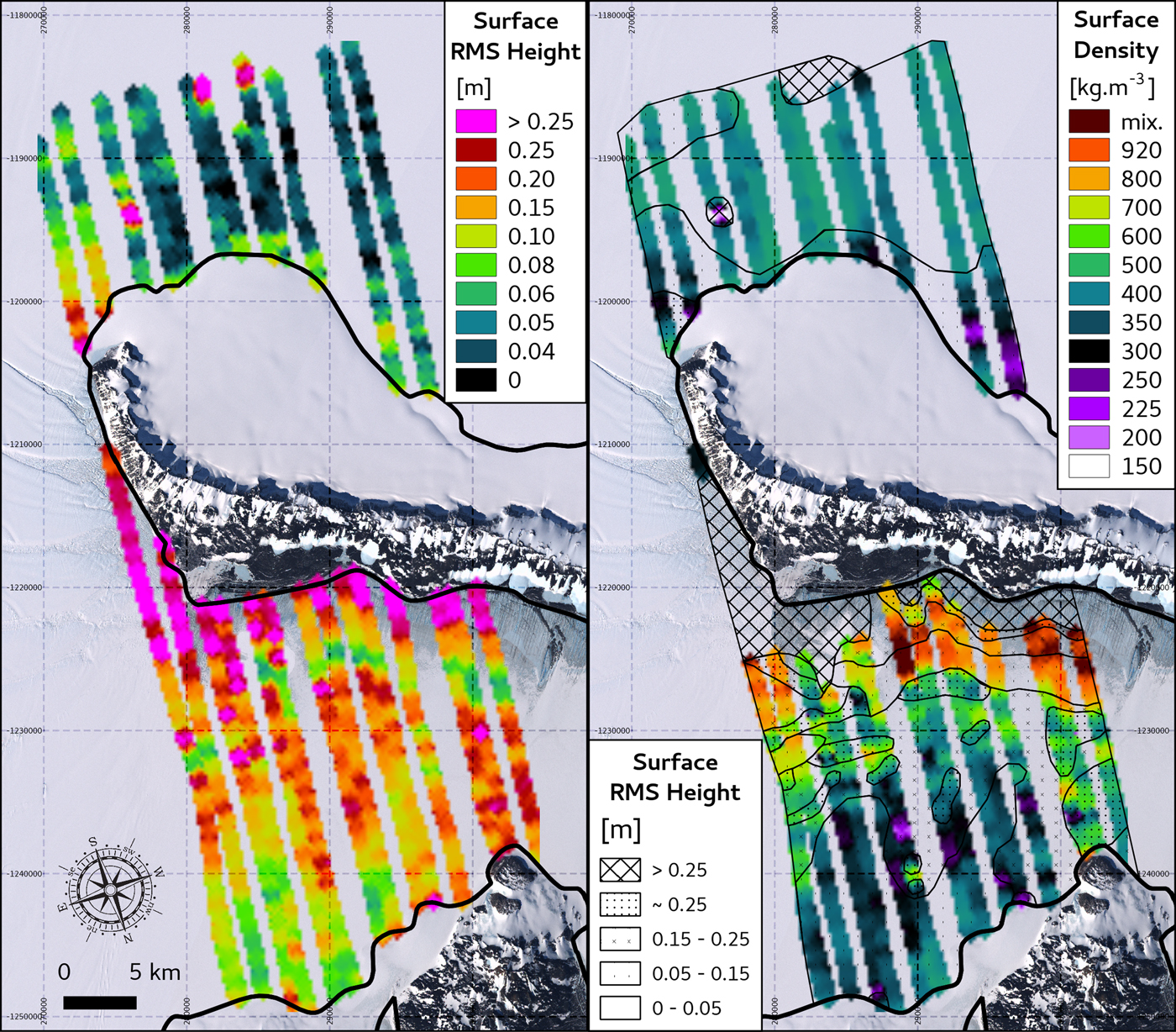
Fig. 3. (Left) Derived surface root-mean-square (RMS) height. Values >0.25 m are beyond the application limits of the backscattering model and are considered underestimated. (Right) Surface density derived where the RMS height is <0.25 m, as allowed by the model's application limits (Grima and others, Reference Grima, Schroeder, Blankenship and Young2014b). The map is superimposed with a classification of the derived surface RMS height for comparison. As for subsequent maps, the background is the Landsat image mosaic of Antarctica (Bindschadler and others, Reference Bindschadler2008) that is superimposed by a 10-km-spaced grid matching the grid on Figure 1 to recover absolute coordinates.
4.1. Surface roughness
Overall, the surface RMS height (Fig. 3. left) appears smoother and more homogeneous over the surveyed portion of RIS, with most values <0.08 m, than the SMIS where the roughness range is mostly >0.08 m and exhibits a more specific pattern. The SMIS surface is rough along the southern edge of Minna Bluff, characterized by elongated ridges several meters in height that run perpendicular to the bluff (Koch and others, Reference Koch, Fitzsimons, Samyn and Tison2015; Koch, Reference Koch2016). This area is also distinguishable as a blue ice area in the Landsat Image (Fig. 1) and coincides with the area where RMS height is >0.25 m. Further to the center of SMIS, the roughness decreases to 0.20 m in line with observations of sastrugi on the ice-shelf surface (Clifford, Reference Clifford2005) and eventually to 0.08 m in the vicinity of White Island. This evolution is not continuous though; at the southern edge of the blue ice area there is a narrow band, about 2 km in width, with a low apparent roughness down to 0.06 m. This area coincides with a change from marine ice exposed at the surface of southern SMIS to meteoric ice (Koch, Reference Koch2016), which is not as dark as the marine ice and thus likely has a higher surface albedo, encouraging less melt in comparison and therefore smoother terrain. Additionally, the occasional seasonal snow cover here is thin enough to hinder sastrugi formation.
4.2. Surface density
The snow and firn density of ice masses at their surface is dependent on overburden pressure, air temperature, relative humidity, and wind redistribution (Kaspers and others, Reference Kaspers2004; Ligtenberg and others, Reference Ligtenberg, Helsen and van den Broeke2011; Grima and others, Reference Grima, Blankenship, Young and Schroeder2014a). The radar-derived density pattern of this study (Fig. 3. right) shows that light snow (< 400 kg · m−3) is gathered in the north and toward the center of SMIS. This matches the density observations from the upper meters of a firn core extracted from northern SMIS (Rosier and others, Reference Rosier2017). SMIS surface density is increasing southward toward Minna Bluff, finally reaching that of compact ice (920 kg · m−3) in its blue ice area where the ice-shelf surface mass balance is negative (Koch, Reference Koch2016), allowing basal marine ice layers to crop out as evident by the ice's composition (Kellogg and others, Reference Kellogg, Kellogg and Stuiver1991; Fitzsimons and others, Reference Fitzsimons, Mager, Frew, Clifford and Wilson2012a; Koch and others, Reference Koch, Fitzsimons, Samyn and Tison2015). The presence of sastrugi in the ice-shelf center (Clifford, Reference Clifford2005) is evidence of high wind velocities, coinciding with firn densities of 400–700 kg · m−3 that likely arise from the wind-packing.
4.3. Marine-to-meteoric ice transition
The smooth band along the marine ice exposure has a similar density, although appearing with an albedo that is indiscernible from the snow-covered part of the ice-shelf on satellite imagery. We interpret this band as marine ice covered by a thin veneer of possibly seasonal and/or wind-blown snow, which is supported by in field ground-based radar and ice sample evidence (Koch, Reference Koch2016). It can also be shown that the limit of the snow-covered part of SMIS can reach further north on Landsat images and varies seasonally. The northern radar limit of the smooth band would then outline the transition between marine ice and meteoric ice. We estimate the thickness of the snow deposit within the smooth band by using a simple three-layer model to quantify the reflectivity losses due to destructive interference from a thin film of snow over ice (Mouginot and others, Reference Mouginot2009). We set the snow layer density to 600-kg · m−3 to equal the average density measured south of the narrow smooth band. We find that for a thickness <0.5 m at the time of acquisition, the snow layer would not produce noticeable coherent losses (less than 3 dB) as observed.
5. BASAL PROPERTIES
The derived basal reflectance and backscattering coefficients, corrected for the measured surface transmission losses and hypothesized homogeneous englacial attenuation as described in Section 3.3, are shown in Fig. 4. As stated in Section 3.4, the basal reflectance and backscatter cannot be unambiguously inverted in terms of basal properties, especially since scattering from roughness and volumic structures might have an equally-dominant incoherent signature. To introduce and support the interpretation of the measured basal coefficients, we propose in the following section a means to provide insights into the physical interpretation of the radar signature in the specific setting of the ice–ocean interface.

Fig. 4. (Left) Basal reflectance, which is mainly dependent on basal permittivity gradient and deterministic structure (e.g., horizontal layering), unless the backscatter is very high. (Middle) Basal backscatter, which is mainly dependent on basal roughness and macroscopic volumic heterogeneities. (Right) The basal coherent content, which is independent of basal permittivity gradient and englacial attenuation, inversely patterns the strength of the geometric heterogeneities at the basal interface (i.e., a low coherent content corresponds to a strong geometric heterogeneities).
5.1. Interpretation insights
Coherent response. Most ice shelves experience a combination of basal ice melting and (re)freezing at the ice–ocean interface (Rignot and others, Reference Rignot, Jacobs, Mouginot and Scheuchl2013a). These processes create structures with different properties that affect the radar signal. A basal reflector that exhibits a strong reflectance together with a high coherent content, for instance, is indicative of a very flat surface with little heterogeneous structures, suggesting an interface smoothed by homogeneous ice melting. Conversely, basal ice accretion usually generates a layer of marine ice with dielectric conductivities that could be more than one order of magnitude higher than that of meteoric ice (Tison and others, Reference Tison, Ronveaux and Lorrain1993), potentially modulating the radar reflectance response to some extent (Pettinelli and others, Reference Pettinelli2015). The recent detection of iron oxide in a marine ice core from Amery Ice Shelf, Antarctica, might be an explanation for such high conductivity (Herraiz-Borreguero and others, Reference Herraiz-Borreguero, Lannuzel, van der Merwe, Treverrow and Pedro2016). The reflectance may also be sensitive to the marine ice layer if its thickness is less than the radar vertical resolution (~6 m in ice). In this case, the ice–ocean interface can be approximated as a thin film stack whose effective reflectance properties are mainly modulated by the marine ice thickness because of signal interferences between the top and bottom reflections of the accreted layer. The conjugated effects of destructive interferences and marine ice attenuation would tend to fade the signal with marine ice thickness increase (Yeh, Reference Yeh1998).
Incoherent response. The structure of accreted ice is expected to be significantly heterogeneous between the Fraunhofer and Rayleigh scales (λ/32 = 0.15 m and λ/8 = 0.62 m, respectively), where radar scattering is boosted and eventually dominates the signal (Ulaby and others, Reference Ulaby, Moore and Fung1981). The formation of accreted marine ice is a bottom-up process starting with the nucleation of suspended frazil ice crystals in supercooled water (Martin, Reference Martin1981; Daly, Reference Daly1984), eventually growing, coalescing, and accumulating at the ice-shelf bottom. Consequently, the first bottom layer of marine ice is usually permeable, and then compacts upward, leading to a medium rich in inclusions such as trapped sea water, along with lithogenic and biogenic debris (Craven and others, Reference Craven2005, Reference Craven, Allison, Fricker and Warner2009; Treverrow and others, Reference Treverrow, Warner, Budd and Craven2010). In this highly compositionally and geometrically heterogeneous medium, the strength of the radar backscatter can be a proxy to the location of frazil/marine ice and possibly also to assess its relative growth maturity.
Ambiguities. Whilst there are few alternatives to ice-shelf basal melting for the formation of a strong and coherent basal reflector, the interpretation of an incoherent return can be ambiguous: a heterogenous basal structure at radar scale could result from cracks or short basal terraces. Basal terraces have been observed at the base of ice shelves associated with Darwin–Hatherton (East Antarctica)(Riger-Kusk, Reference Riger-Kusk2011), Pine Island (West Antarctica), and Petermann (Greenland) (Dutrieux and others, Reference Dutrieux2014) glaciers, as well as at northern SMIS (Ryan, Reference Ryan2016) together with basal crevasses (Rosier and others, Reference Rosier2017). On radargrams, such terraces usually appear as a series of periodic bent steps arranged perpendicular to an ice thickness gradient and separated by an abrupt near-vertical wall. Although their radar character is not incompatible with crevasses from mechanical origins, differential basal melting from ascending meltwater formed at the grounding line is usually favored as the driving process (Dutrieux and others, Reference Dutrieux2014).
5.2. Basal reflectance and backscatter
Basal reflectance and backscatter (Fig. 4) exhibit both meaningful and very specific patterns that we will attempt to classify and interpret in the following. The basal reflectance shows a distinct pattern, whereby the center of SMIS has higher values (between − 12 and − 7 dB) than around its edges in the northeast, east, and south. The basal backscatter is lowest in the northeast portion of SMIS and decreases gradually toward its center. A more abrupt change from around − 1 to − 15 dB occurs between the northeast and the center-east of the ice-shelf, adjacent to the shear zone to RIS. The basal coherent content is lowest (− 30 to − 10 dB) in its north and varies between − 6 and 5 dB in its center. Around its eastern and southern margins, the basal coherent content drops again to − 20 to − 10 dB. Echo-free (EF) zones (e.g., without distinguishable reflector following the surface) are also identified within SMIS.
Remarkably, the reflectance and backscatter basal properties sharply change at specific depths over both RIS (at about 440 and 580 m) and SMIS (at about 105 and 200 m) as seen in Fig. 5a-b. Here, the ice thickness is related to the depth of the basal reflector below the surface not the absolute depth below sea-level, which needs hydrostatic correction. We hypothesize that these sharp backscatter gradients are isolines at which the pressure melting point is reached because they occur along specific depths and they delineate units dominated alternatively by scattering and reflectance, as expected by melting and freezing processes respectively. The temperature of the pressure melting point and its associated location along the ice–ocean interface of the ice-shelf base is mainly driven by local ocean salinity, the thermohaline circulation pattern, and the actual interface depth (e.g., Galton-Fenzi and others, Reference Galton-Fenzi, Hunter, Coleman, Marsland and Warner2012; Gwyther and others, Reference Gwyther, O'Kane, Galton-Fenzi, Monselesan and Greenbaum2018).
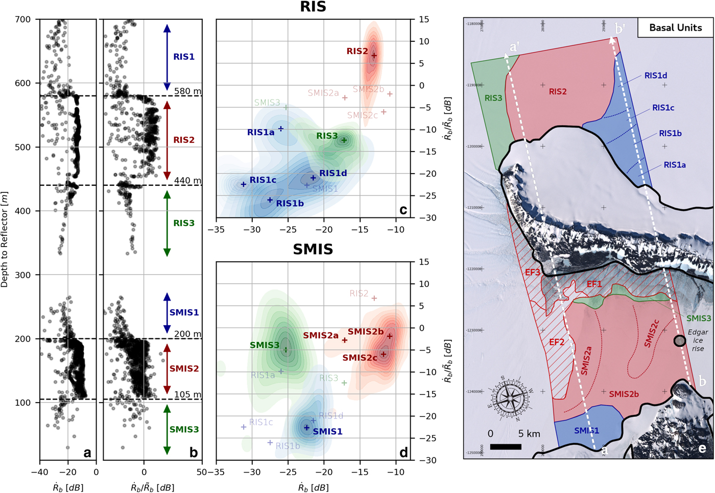
Fig. 5. Basal reflectance (a) and basal coherent content (b) as a function of depth to the related reflector for both RIS and SMIS. On a first approach, the behavior of these properties can be classified into various regimes sharply transitioning around specific depths (105, 200, 440, 580 m), delimiting six main units (RIS1-3 and SMIS1-3). A kernel density estimation of the distribution of the same data set in the reflectance vs coherent content space is shown for RIS (c) and SMIS (d). It supports identifying various sub-units with the joint use of Figure 4. Interestingly, while the main units are delimited by various depths, sub-units are not. The identified basal units are located on (e), also showing the radargram groundtracks from Figure 6 (dotted white lines).
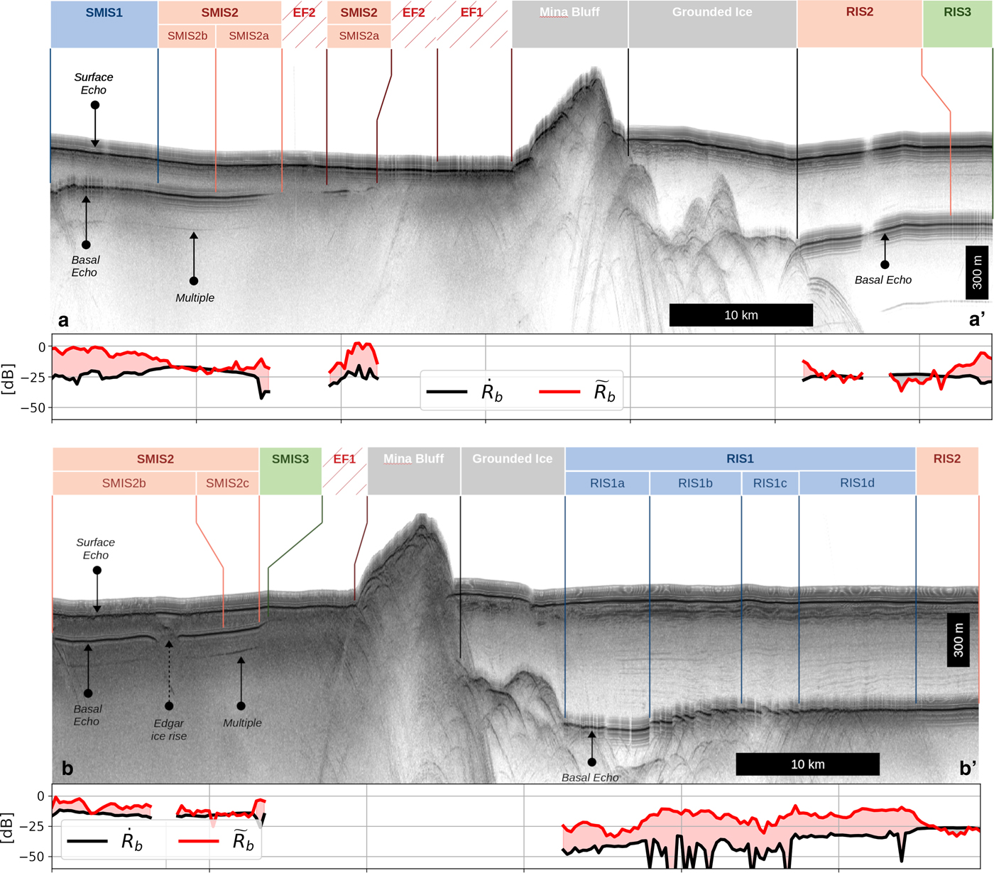
Fig. 6. HiCARS2 radargrams across the studied region, corresponding to the ground tracks shown in Fig. 5e. The primed letters of the cross-section naming are southward. The extent of the derived basal units are also highlighted. The horizontal and vertical scales are indicative only; they might vary slightly locally due to differential aircraft speed and surface range along each track. Below each radargram is plotted with the same identical horizontal scale the bed reflectance (black) and backscatter (red). The amplitude difference (color-filled area) between the two curves is indicative of the coherent content.
Here, we propose that a sharp gradient delimiting a high-to-low ${\dot R}_{\rm b}/\tilde {R_{\rm b}}$ ratio is a boundary between a melting and freezing ice–ocean interface, respectively, as the latter should be characterized by a growing non-deterministic structure responsible for a stronger signal backscatter. Thus, this technique provides insights for determining the location of the pressure melting point at the ice-shelf base.
5.3. Basal units
The detected ice thickness depth isolines matching a sharp modification in the radar properties are used to outline six main units (RIS1-3 and SMIS1-3) whose specific radar signatures and interpretations are discussed below. Within some of these units, additional sub-units (RIS1a-b and SMIS2a-c) can be distinguished, but their boundaries do not obviously match depth isolines. These sub-units are also discussed in the following paragraphs. Additionally, echo-free zones (EF1-3) where no basal detection occurs are also discussed. The radar properties of all the described units are gathered in Figure 5. C-D in the form of a two-parameter space plot classifying the units in terms of their ${\dot R}_{\rm b}$ and ${\dot R}_{\rm b}/\tilde {R_{\rm b}}$
 coefficients. The location of each unit is shown in Figure 5e, and a pair of illustrating radargrams is given in Figure 6.
EF1-3. An echo-free (EF) zone defines a unit where no subsurface return is detected below the surface echo. We have divided the EF zones into three units for which satellite imagery helps define different hypotheses that explain the absence of basal reflection. Within EF1, Landsat imagery outlines a wide field of blue ice identified by in situ ice samples mostly as a marine ice outcrop (Kellogg and others, Reference Kellogg, Kellogg and Stuiver1991; Koch and others, Reference Koch, Fitzsimons, Samyn and Tison2015). The absence of a basal reflector can be explained by signal attenuation within the thick and highly conductive marine ice column (Pettinelli and others, Reference Pettinelli2015). EF2 marks the boundary between RIS and SMIS perpendicular flows (Clifford, Reference Clifford2005; Koch, Reference Koch2016). The Landsat imagery does not distinguish EF2 visually from the surrounding white surface snow, which characterizes most ice shelves. We hypothesize EF2 to be a prolongation of the EF1 thick marine ice, but blanketed by a snow layer as described in Section 4.3. For EF3, the satellite imagery shows numerous crevasses and disrupted ice as also detected with ground-based ice penetrating radar (Arcone and others, Reference Arcone2016), in line with an area of high stress rates. Marine ice is also likely present here (Arcone and others, Reference Arcone2016). In this configuration of a rough and disordered media, the absence of basal detection could be explained by strong signal scattering, complemented by attenuation from conductive marine ice pockets within fractures.
RIS1. This is the deepest detected unit (below 580 m). Overall, RIS1 is characterized by the weakest radar reflectance and reflectance/backscatter ratio of our data set, suggesting an area dominated by heterogeneous structures below radar scales. However, four sub-units (RIS1a-d) corresponding to the basal morphology trend indicate subtle basal variations. RIS1a radar properties stand out from its counterparts and a specific basal process cannot be ruled out here. Its stronger coherent content is indicative of a flatter interface. However, RIS1a's low reflectance is somewhat similar to that of RIS1b-d. This combination could be explained by localized basal melting where englacial attenuation has been overestimated (Matsuoka and others, Reference Matsuoka, MacGregor and Pattyn2012), thus lowering the perceived reflectance; or by the presence of a thin basal marine ice layer that would weaken the signal return by destructive interference. A melting hypothesis appears more likely in the usual scheme of cavity circulation where melting occurs at the deepest layer, close to the grounding line, and water becomes supercooled as it rises into thinner areas (Lewis and Perkin, Reference Lewis and Perkin1986). Note that the hyperbolas around RIS1a's northern-half suggest proximity to the bedrock and grounding/floating transition.
The morphological character of RISb-d (Fig. 6b-b') is consistent with a basal-step setting with terraces up to 1-km long within RIS1b, where the base is the steepest. The terraces appear shorter in RISc and eventually fall below radar resolution in RIS1d where the base flattens but scattering hyperbolas from corner reflectors are still visible. This suggests that the basal step dimensions and formation processes are scaled by the basal slope. There are few and faint englacial layers distinguishable above RIS1b-c. Their apparently disturbed morphology suggests a foliation that could come from compression of the buttressed ice-shelf, locally thickening the ice and leading to a basal slope where the process responsible for the basal steps could initiate. However, a better resolved radar investigation might be necessary in this area to confirm the layer morphology. The englacial layers above RISd appear to bend downward, eventually intersecting the ice/ocean interface, and supporting a negative basal mass balance sustained by melting. However, the weak RISb-d radiometric properties are typical of what could be expected from ice accretion. A possibility for these sub-units is to have melting further north, closer to the grounding line, with subsequent melt water migration to shallower depths.
RIS2. This unit has the strongest reflectance/backscatter ratio (+ 6.3 dB) and one of the highest reflectances of the defined units. Both measurements together are a strong signature of what could be expected from a wide and flat field of basal melting. The relatively steady reflectance across the unit supports the hypothesis of a highly deterministic interface. Note that a narrow 1-km band of low reflectance (visible on Fig. 4) is present along the coast line in the vicinity of the grounded Minna Bluff Glacier. This band might be attributed to the grounding/floating ice transition with the presence of bedrock scattering.
RIS3. The radar properties of the basal reflectors get notably weaker from RIS2 to RIS3. The alternation of melting/freezing processes at ice-shelf's base suggests that RIS3 might be a region of ice accretion that follows the suggested melting in RIS2. The thinner RIS would allow traveling of ice-shelf water to these shallower heights and an associated loss of overburden pressure allowing for supercooling of the water mass and thus frazil ice formation. The possibility of scattering from a basal-step setting similar to RIS1 is unlikely since such a basal character does not appear on the radargram in Figure 6a-a'. In particular, the base at RIS3 is continuous and does not exhibit any scattering hyperbolas that seem to accompany basal steps at RIS1.
SMIS1. A basal-step setting has been previously detected at SMIS1 with a higher-frequency ground radar (Ryan and Christensen, Reference Ryan and Christensen2012). The steps are too small to be well resolved by HiCARS2, but the existing ice thickness gradient (Fig. 6a-a'), together with the weak radiometric properties quasi-similar to RIS1d, suggest that SMIS1 is amenable to basal step formation. Note that sub-unit identification within SMIS1 is not as obvious as compared to RIS1. This is probably due to its smaller extent, at the threshold of the RSR technique horizontal resolution.
SMIS2. This unit has complex radar properties. The basal reflectance does not exhibit sharp gradients and has an overall strength more similar to inferred melting ice (e.g., RIS2) than freezing ice (e.g., RIS3). A steady southward increase of the reflectance suggests a progressive modification of the deterministic composition/structure of the ice–ocean interface. As discussed in Section 5.1, such an effect could be caused by an increasing permittivity gradient and/or the presence of a <6 m marine ice layer thinning toward Minna Bluff.
SMIS2a is a sub-unit bordering EF2 over a 3-km wide band where both the basal reflectance and scattering are weak. We propose SMIS2a to be a transition unit where the marine ice content within the vertical ice column is rapidly decreasing westward from EF2. The marine ice is likely generated as the ice-shelf water ‘climbs’ from the RIS cavity into the much thinner SMIS cavity (Koch and others, Reference Koch, Fitzsimons, Samyn and Tison2015).
The rest of SMIS2 has a coherent content behavior that differs from the reflectance map. We distinguish two additional sub-units with specific reflectance and backscatter properties, SMIS2b-c, as 3-km wide bands somewhat perpendicular to the thickness gradient, but parallel to ice-shelf flow (Clifford, Reference Clifford2005; Koch, Reference Koch2016). Together, EF2 and the bands formed by SMIS2a-c appear to be more-or-less arranged radially from SMIS1. We propose three hypotheses to account for this setting:
(1) As for RIS1, thermohaline circulation gradients could be responsible for an active east-west differential marine ice growth/decay across the unit, or possibly non-mature frazil ice. However, such an ice accretion trend, which is not correlated with the ice thickness gradient, is hard to reconcile with the observed perpendicular reflectance variation that we postulated for a progressive evolution in maturity of accreted marine ice content.
(2) In contrast to active accretion at present day, SMIS2b-c could be relics of former differential basal mass balances upstream of the ice-shelf flow, possibly originating from the EF2 location. The SMIS flow velocity does not exceed 6 m · a−1 at its heart according to GPS measurements (Clifford, Reference Clifford2005). Given that the bands formed by SMISb-c are up to ~4 km wide, and assuming a constant ice-shelf velocity over time, it would indicate a basal mass balance variability over a ~ 700 year timescale. However, this hypothesis would require a recent and drastic change in the basal accumulation rate given that today's echo-free zone EF2 suggests much thicker marine ice than the thin layer variability that was hypothesized for SMIS2a, unless SMIS2b-c is melting and eroding the marine ice thickness previously accreted upflow.
(3) SMIS2a might be a marine ice accretion prism in the continuity of EF2, similar to, but not as abrupt as, SMIS3 and EF1, respectively. Then, SMIS2c could simply be explained by a different ocean circulation regime influenced locally by the Edgar Ice Rise located in center-west SMIS (see Fig. 5e), which is a vertical bedrock intrusion locally grounding the ice and on which the ice-shelf is buttressing (Clifford, Reference Clifford2005; Rack and others, Reference Rack, King, Marsh, Wild and Floricioiu2017; Wild and others, Reference Wild, Marsh and Rack2018). This pinning point can be easily identified on the HiCARS2 radargrams (Fig. 6b-b').
SMIS3. This unit is a narrow feature between EF1 and SMIS2 geometrically characterized by a sudden decrease in the ice thickness (Fig. 4) and associated steep basal reflectors, in contrast to the gentle slope of SMIS2 (Fig. 6b-b'). Although its weak reflectance is similar to RIS1, its strong coherent content is a signature of a deterministic flat interface. Bundled together, these properties likely indicate a meteoric/marine interface for which the dielectric gradient is known to be far lower than for an ice–ocean interface (Pettinelli and others, Reference Pettinelli2015). This argument is supported by the known exposure of marine ice at the ice-shelf surface within the adjacent EF1. Such a setting accommodates the ice-shelf vertical structure proposed by Koch (Reference Koch2016) from ground radar observations. In that scenario, the slope break in the basal reflector delimiting SMIS2 from SMIS3 (Fig. 6) would indicate the location where the thickness of accumulated marine ice exceeds the radar vertical resolution. The marine ice column would then grow southward until surface exposure.
6. CONCLUSIONS AND PROSPECTS
Ice shelves are crucial regulators of the grounded ice flow into the ocean for two-thirds of the Antarctic ice sheet through buttressing at passive margins and local pinning points (Bindschadler and others, Reference Bindschadler2011). Ice-shelf disruption accelerates the transfer of land ice into the ocean that will eventually melt and contribute to sea level rise (De Angelis and Skvarca, Reference De Angelis and Skvarca2003; Scambos and others, Reference Scambos, Bohlander, Shuman and Skvarca2004). The assessment of ice-shelf stability requires a knowledge of the boundary conditions at both their surface and basal (i.e., ice–ocean) boundaries (Gwyther and others, Reference Gwyther, Galton-Fenzi, Dinniman, Roberts and Hunter2015). Firn density, ice composition, and geometric structure (e.g., roughness) are all properties scaled by the processes contributing to the ice shelves mass balance at these boundaries, making them important observables to assess ice-shelf stability. However, global climate models and continental data sets rendering the surface properties do not account for the local singularities that might better explain the behavior of a regional catchment (e.g., Grima and others, Reference Grima, Blankenship, Young and Schroeder2014a; Cook and others, Reference Cook, Galton-Fenzi, Ligtenberg and Coleman2018). Likewise, constraining basal boundary conditions in situ is logistically challenging, while access through ice coring provides only a sparse sampling of an entire ice-shelf (Oerter and others, Reference Oerter1992; Tison and others, Reference Tison, Ronveaux and Lorrain1993; Treverrow and others, Reference Treverrow, Warner, Budd and Craven2010), although core site locations can be supported by ground penetrating radar with limited range deployment.
Our analysis focused on SMIS and a portion of the RIS. SMIS is separated from RIS by a rift zone and exhibits a heterogeneous ice composition made of both marine and meteoric ice (Kellogg and others, Reference Kellogg, Kellogg and Stuiver1991; Fitzsimons and others, Reference Fitzsimons, Mager, Frew, Clifford and Wilson2012b; Koch and others, Reference Koch, Fitzsimons, Samyn and Tison2015), suggesting a complex mass balance where both surface and basal processes compete equally. We used ice penetrating radar data obtained in a 2014–15 austral summer airborne survey and developed a methodology to extend the application of the RSR technique from the surface to the basal radio properties at a scale relevant to detect local singularities that might play a critical role in ice-shelf mass balance.
The surface radar properties are inverted in terms of surface snow density and root-mean-square heights, leading to a distribution pattern of the processes contributing to the surface boundary conditions that are compatible with the observed marine ice exposure along Minna Bluff. We locate the transition between the marine ice exposure and the meteoric ice, below a thin <0.5 m layer of fresh snow at the time of survey.
The ratio of the RSR-derived basal reflectance and backscatter coefficients provides the basal coherent content, a measurement of the geometric disorder at the ice–ocean boundary that is corrected for both surface transmission losses and englacial attenuation. The basal radar properties exhibit sharp and strong gradients along specific iso-depths, suggesting an abrupt modification of the ice composition and geometric structure at the ice–ocean boundary. We argue that this behavior demonstrates RSR identification of locations where the pressure-melting point is reached. Our framework for classifying basal radiometric properties further sheds light on basal boundary condition patterns and their related processes, driven mainly by the freezing and melting of ice. For example, basal steps are observed at both SMIS and RIS, suggesting a common geometric expression of some basal processes hypothesized to be driven by ascending meltwater formed at the grounding line (Dutrieux and others, Reference Dutrieux2014).
Future directions include addressing ambiguities that remain for interpretation of the basal radio properties. This could be achieved by, first, better understanding of the spectra of dielectric properties and geometric structures offered by frazil ice and refrozen marine ice with brine inclusions, and second, by further quantifying the interactions of radio waves with these media.
Terrestrial ice-shelf cavities also provide a unique and accessible analog for ice-covered ocean worlds in the solar system. For example, the salinity and pressure at the basal boundaries of terrestrial ice shelves is comparable to what is expected at Europa (Blankenship and others, Reference Blankenship, Young, Moore and Moore2009), the Jovian icy moon that may harbor conditions suitable for life (Reynolds and others, Reference Reynolds, Squyres, Colburn and McKay1983). As for Earth, the accretion of frozen marine ice at the ice/ocean interface of Europa can act as a mechanism for trapping ocean material (Craven and others, Reference Craven2005; Howell and Pappalardo, Reference Howell and Pappalardo2018), including possible relics of an active habitat, while its distribution is an indicator of ocean circulation (Soderlund and others, Reference Soderlund, Schmidt, Wicht and Blankenship2013).
Europa is the target of NASA's upcoming Europa Clipper mission (Phillips and Pappalardo, Reference Phillips and Pappalardo2014) to be launched in the early 2020s to investigate the satellite's habitability. The Radar for Europa Assessment and Sounding: Ocean to Near-surface (REASON) instrument, a multi-frequency, multi-channel ice penetrating radar system with a VHF band that is similar in frequency and bandwidth to HiCARS2, could revolutionize our understanding of Europa's ice shell by providing the first direct measurements of its surface character and subsurface structure. The techniques developed here will provide an exciting new data analysis approach for characterizing the surface and basal boundary conditions along the ice–ocean interface as well as any liquid water lenses embedded within the ice shell (Schmidt and others, Reference Schmidt, Blankenship, Patterson and Schenk2011).
ACKNOWLEDGMENTS
This work was supported by the G. Unger Vetlesen Foundation. CG and DMS were supported, in part, by grant #NNX16AJ95G from the NASA Cryospheric Sciences Program. IK was supported by ICIMOD's Cryosphere Initiative funded by Norway, and by core funds of ICIMOD contributed by the governments of Afghanistan, Australia, Austria, Bangladesh, Bhutan, China, India, Myanmar, Nepal, Norway, Pakistan, Sweden, and Switzerland. We are very grateful for a SCAR/COMNAP Fellowship that sponsored a research stay of IK at UTIG. We acknowledge the Norwegian Polar Institute's Quantarctica package. This is UTIG contribution #3458.


 Open access