


Introduction
A largely neglected field of glaciological research is the calving dynamics of glaciers and ice sheets along the fronts of grounded ice walls and floating ice shelves. Yet, calving into the sea is the dominant ablation mechanism of the Antarctic ice sheet and a major ablation mechanism of the Greenland ice sheet. Calving was also a major factor in the retreat of marine (Reference HughesHughes, 1977; Reference Andersen, Denton and HughesAndersen, 1981; Reference Mayewski, Denton, Hughes, Denton and HughesMayewski and others, 1981) and lacustrine (Reference AndrewsAndrews, 1973; Reference HughesHughes, 1987; Reference Teller, Ruddiman and WrightTeller, 1987; Reference GrosswaldGrosswald, 1988) margins of Northern Hemisphere ice sheets during the last deglaciation. In modeling Antarctic deglaciation, ice-calving rates had to be parameterized in rather arbitrary ways because little was known about calving dynamics, yet calving rates are a critical constraint on retreat rates in the models (Reference Thomas and BentleyThomas and Bentley, 1978; Reference Stuiver, Denton, Hughes, Fastook, Denton and HughesStuiver and others, 1981; Reference Fastook, Hansen and TakahashiFastook, 1984).
Attempts to understand the interaction between glaciation and climatic change cannot afford to ignore calving dynamics (Reference Paterson, Hammer, Ruddiman and WrightPaterson and Hammer, 1987). Nor can calving dynamics be ignored in modeling simulations of deglaciation and rising sea level in response to “greenhouse” warming over the next few decades, as fossil fuels are consumed. In this context, calving dynamics are particularly important for the fast ice streams that discharge upwards of 90% of Antarctic and Greenland ice into the sea. Moving 7 km a−1 along its calving front (Reference Echelmeyer and HarrisonEchelmeyer and Harrison, 1990), Jakobshavns Isbras (69.2° N, 49.9° W) is the fastest known ice stream, and its calving rate equals its velocity (Reference Pelto, Hughes and BrecherPelto and others, 1989). Rapid calving rates are part of the Jakobshavns effect, a series of positive feed-backs for rapid deglaciation of Jakobshavns Isbrse, in which ice-stream flow produces a heavily crevassed surface, allowing summer surface meltwater thermally to soften deep ice and lubricate the bed, thereby increasing velocity, crevassing, melting and calving, in that order (Reference HughesHughes, 1986). Since 1964, retreat of the calving front linked to those feed-backs has been halted near the headwall of Jakobshavns Isfjord, but what if “greenhouse” warming produces this “Jakobshavns effect” of fast velocity and calving in all Greenland and Antarctic ice streams with no fiord headwalls (Reference HughesHughes, 1987). The Jakobshavns effect can be defined as deglaciation of marine ice-sheet margins by rapid calving, so that ice melting is accomplished primarily by floating icebergs to warmer ocean waters, instead of by bringing atmospheric warmth to the ice sheet.
Enough is known about calving dynamics to realize the complexity of this glaciological process. Reference ReehReeh (1968) made the first theoretical analysis of calving along the floating fronts of glaciers, using calving from Jakobshavns Isbrae, as reported by Reference Carbonnell and BauerCarbonnell and Bauer (1968), to test his theory that calving resulted from bending stresses induced by the imbalance of hydrostatic forces in ice and water at the calving front. His results predicted maximum tensile bending stresses about one ice thickness behind the calving front, which was compatible with the observation that tabular icebergs were of about these proportions. Reference Fastook and SchmidtFastook and Schmidt (1982) developed a finite-element model that duplicated these results and extended them to include enhanced calving along water-filled crevasses. Scattered crevasses on Jakobshavns Isbrae are filled with water, but none reach the calving front in that condition.
(Reference HoldsworthHoldsworth 1969, Reference Holdsworth1971, Reference Holdsworth1973, Reference Holdsworth1974, Reference Holdsworth1977, Reference Holdsworth and Jacobs1985) has made detailed theoretical and observational analyses of flexure along the grounding line of floating glaciers, caused by tidal and wave action, as a mechanism for releasing very large tabular icebergs. Other studies of this mechanism were by (Reference RobinRobin 1958, Reference Robin1979), Reference Hughes, Parkinson, Brecher and Gonzales FerranHughes (1976), Reference Lingle, Hughes and KollmeyerLingle and others (1981), (Reference Holdsworth and GlynnHoldsworth and Glynn 1978, Reference Holdsworth and Glynn1981) and Reference Vinogradov and HoldsworthVinogradov and Holdsworth (1985). Reference HughesHughes (1983) has argued that large tabular icebergs would be released from floating ice shelves along lines of weakness that formed from rifts alongside ice streams that supplied the ice shelf and from gashes through the ice shelf in the lee of ice rises, in addition to flexure along ice-shelf grounding lines, and that these lines of weakness divided an ice shelf into plates that were potential tabular icebergs long before the plates reached the calving front. Wordie Ice Shelf in the Antarctic Peninsula seems to be disintegrating along these lines of weakness at the present time (Reference Doake and VaughanDoake and Vaughan, 1991).
Reference IkenIken (1977) made the first theoretical study of slab calving from an ice wall undercut along the shoreline of a beach. She assumed homogeneous deformation based on continuum mechanics to conclude that slabs were about as thick as the height of the ice wall. Reference HughesHughes (1989) reported non-homogeneous deformation in an ice wall on Deception Island (63.0° S, 60.6° W), from which slabs having much less thickness calved along shear bands caused by a bending moment at the base of the ice wall.
This mechanism was later observed to be dominant for glaciers entering water in the Chilean Andes and along the Antarctic Peninsula, even when the ice wall was undercut along the water line by wave action (Reference Hughes and NakagawaHughes and Nakagawa, 1989). A theoretical formula derived for this mechanism on Deception Island had a summer calving rate proportional to the inverse square of the ice-wall height. A summer calving rate inversely proportional to the square of ice height above ice height supported by water buoyancy was reported for the ice wall of Columbia Glacier by Reference Brown, Meier and PostBrown and others (1982), who also observed an annual calving rate proportional to water depth for 12 Alaskan tide-water glaciers, including Columbia Glacier. These calving relationships were also discussed by Reference MeierMeier and others (1980), Reference SikoniaSikonia (1982) and by Reference Bindschadler and RasmussenBindschadler and Rasmussen (1983).
Studies of calving dynamics, whether slab calving from ice walls or tabular calving from ice shelves, are a neglected part of glaciology largely because of dangers inherent in calving environments, especially calving into water. The mobility of field workers is severely limited along marine and lacustrine calving ice margins, and calving from ice cliffs up to 100 m or more above water level is unpredictable and can be frequent. Our detailed studies of calving dynamics on Deception Island were possible only because the calving ice wall was standing on dry land and solifluction of a thick ash layer on the glacier surface had produced a series of ash ramps that gave us safe access to various heights along the ice wall (Reference Brecher, Nakagawa and HughesBrecher and others, 1974; Reference Hughes, Parkinson, Brecher and Gonzales FerranHughes and others, 1974; Reference HughesHughes, 1989; Reference Hughes and NakagawaHughes and Nakagawa, 1989).
Theory
Direct observations of the calving ice wall on Deception Island, including tunneling into the wall at various heights, revealed numerous shear bands that rose vertically from the bed behind the ice wall and curved increasingly forward with increasing distance above the bed, so that shear displacement increased from zero at the bed to a maximum at the surface (Reference HughesHughes, 1989). Some of these shear bands are shown in Figure 1. Non-homogeneous bending creep produces the shear bands, and shear in them is similar to the slip between pages of a book when the book is bent about its binding.

Fig. 1. Shear bands on the Deception Island (63.0° S, 60.6° W) ice wall revealed by vertical offsets of ash layers in the ice. Access to the ice wall was by ash ramps of various heights, one of which is in the background.
Shear rupture across a shear band leads to the kind of slab calving shown in Figure 2. Shear rupture in a shear band at calving distance c behind the ice wall opens a crevasse that removes coupling of the slab to the glacier. As the crevasse deepens, the entire weight of the slab must be borne by ice at the base of the slab, and by ice below the crevasse tip that still connects the slab to the glacier. If the basal ice is crushed by the ice load above it, the slab will crash vertically downward. If the crevasse widens as it deepens, the slab will continue to bend until it topples forward. Let θ be the angle of forward bending for the ice slab. The slab will collapse downward when θ and c are small, because the crushing stress is high, and topple forward when θ and c are larger, because the bending stress is high. An overhanging ice wall is therefore necessary for forward calving but not for downward calving. In Figure 2, the ice wall looks like it could calve either way. The slab bends forward at θ ≈ 18° from the vertical and the crevasse formed at c ≈ 0.4h behind the wall, where h is the wall height. This combination of θ and c\h, therefore, may be close to the transition from downward calving to forward calving. There is no special significance in this transition.

Fig. 2. A slab about to calve from the ice wall of an Antarctic glacier (photograph by D. Allan).
The mechanics of slab calving used here will be based on the theory for bending beams, as presented by Reference PopovPopov (1952) with appropriate modifications. Reference PopovPopov (1952, p. 89) listed the eight steps in beam analysis needed to determine the shear force, the axial force, and the bending moment at any cross-section of a beam. An initially vertical beam of ice resting on the bed will be considered. The beam has length c, width w and mean height h. In general, an ice wall stands in water, so distributed loads of ice and water act on opposite sides of the beam, causing the beam to bend forward. As shown in Figure 3, when water of depth d rises against a wall of height h, increasing buoyancy decreases basal shear stress τ0, thereby causing a reduction of surface slope α, such that τ0 and α approach 0 when the ice wall begins to float at d = (ρI/ρw)h, where ρI and ρw are ice and water densities, respectively, and are assumed to be constant. Questions to be examined are whether θ and c depend on d and h, and how calving rate uc depends on θ, c, d and h. Specifically, an approximate calving rate that depends on these variables will be derived.

Fig. 3. The effect of water depth on an ice wall. Arrows show the difference between the lithostatic pressure in ice and the hydrostatic pressure in water (sloping dashed lines). This pressure difference, basal shear stress τ0, surface slope α, and perhaps slab-size decrease as water deepens, with τ0 α = 0 at flotation depth, when tabular calving replaces slab calving.
Step 1 consists of producing a free-body diagram in which all forces acting on the beam, taken as the slab that will calve, are referenced with respect to orthogonal coordinates. Figure 4 presents the diagram. The origin of Cartesian coordinates is on the bed at calving distance c behind the ice wall, with x horizontal and positive forward, y horizontal and parallel to the wall, and z vertical and positive upward. Action forces are the distributed horizontal lithostatic force of ice F I on the left side of the slab, the distributed horizontal hydrostatic force of water Fw on the right side of the slab, and the vertical body force F B of the slab itself. These are all gravitational forces, with g being gravity acceleration. Good approximations for dynamic equilibrium are:
where ½ρIghc is the mean lithostatic pressure pushing on area whc for ice thickness hc at calving distance c,
where ½ρwgd is the mean hydrostatic pressure pushing on area wd for ice thickness h at the ice wall and
where ![]() is the average slab height, wch
is the slab volume and wcd is the water volume it displaces.
is the average slab height, wch
is the slab volume and wcd is the water volume it displaces.

Fig. 4. Free-body diagrams for a slab at an ice wall before shear rupture detaches the slab. Left: boundary conditions; right: forces and moments.
Step 2 consists of adding reaction forces to the freebody diagram. As located in Figure 4, these are a vertical basal normal force F N, a horizontal basal traction force F 0, a vertical shear force F S and a horizontal tensile force FC that opens the crevasse at c:
where horizontally averaged basal axial stress σzz acts through the substrate normal to basal area wc,
where horizontally averaged basal shear stress τ0 acts parallel to basal area wc,
where vertically averaged bending shear stress τs induced by F S acts parallel to calving area whc , and
where vertically averaged axial stress σxx acts normal to calving area whc.
Step 3 consists of measuring moment lever arms L I, L W, L B,L N, L O, L S and L C, parallel to axes x,z for forces F I, F W, F B, F N, F O, F S, and F C, respectively, for bending moment M Y , where:
These are all shown in Figure 4. Equations (10) is exact only if the surface and bed are parallel.
Step 4 consists of applying the equations of statics to compute unknown reaction forces, assuming no inertial forces. Force equilibrium along x requires that:
from which, up until a tensile crack opens the shear band:

Force equilibrium along z requires that:
from which:

Moment equilibrium about the Y-axis requires that, up until a tensile crack opens the shear band:
from which:

where bending moment My causes bending creep at cross-section whc that leads to shear rupture and crevassing in the shear band at calving distance c from the ice wall.
Step 5 consists of specifying the forces at cross-section whc . Axial force F c is obtained from Equation (7) and (14):
Shear force F s is obtained from Equation (6) and (16):
Force F s causes shear rupture in the shear band and force F c causes the shear band to open into a crevasse.
Step 6 consists of isolating the slab after the crevasse opens and showing the forces and bending moments acting on it immediately prior to calving. As seen in Figure 2, the crevasse can separate most of the slab before it actually calves. The free-body diagram for the ice slab at this stage of bending creep is shown in Figure 5.

Fig. 5. Free-body diagrams for a slab at an ice wall after shear rupture detaches the slab. Left: boundary conditions; right: forces and moments.
Step 7 consists of major changes in the action and reaction forces if some assumptions are made. First, assume a thawed bed allows water to fill the crevasse to depth d, so that:
Secondly, downward penetration of the crevasse stops when σxx = 0 at the crevasse tip, so that:
Thirdly, bending creep in numerous shear bands through length c has inclined the ice slab an angle θ from the vertical, with θ increasing along z. Figure 6 shows similar triangles for which θ is the angle formed by the z-axis and the distance vector to point x,z on the bending curve, and by velocity vectors u x and u z of point x,z. Therefore:
where forward displacement x of the slab increases along z, with point x,z on the slab having forward velocity u x and downward velocity u z due to bending creep.

Fig. 6. A bending ice slab after τs has caused shear rupture in a shear band and σxx has opened a crevasse along the ruptured shear band. The relationship between the angle θ in the crevasses, point x,z on the slab side of the crevasse and velocities ux,uz at point x,z is shown geometrically and is given by Equations (23). Note that ux = uc at the top of the crevasse.
Step 8 consists of solving the equations of static equilibrium for the free body in Figure 5. No net horizontal forces are present. Summing vertical forces:
Summing bending moments:
where s is horizontal bending displacement x at height ![]() of the centroid of the slab. Therefore, from Equations (23):
of the centroid of the slab. Therefore, from Equations (23):
Entering Equation (3) and (4) into Equations (24) gives:
Combining Equations (24) through (27) gives:
A calving criterion can be developed for the slab by entering My into the flexure formula (Reference PopovPopov, 1952, p. 98102), and then deriving the differential equation for bending (Reference PopovPopov, 1952, p. 269–73).
In deriving the flexure formula, bending stresses normal to the beam cross-section, tensile on the convex side and compressive on the concave side, create an internal bending moment that exactly resists the external bending moment (Reference PopovPopov, 1952). The important concepts used to derive the flexure formula are: (1) beam geometry which establishes the variation of strain in the beam cross-section, (2) beam rhcology which relates strain to stress, and (3) the laws of statics which locate the neutral axis and resisting moment at the beam cross-section. The flexure formula usually assumes elastic bending only, so that Hooke‘s law can be used to relate stress to strain. In this case, the flexure formula can be used to derive the differential equation for the elastic bending curve for a beam in static equilibrium (Reference PopovPopov, 1952, p.269–73). When beam height h along z is large compared to beam length c in bending direction ι and beam width to, a good approximation is:

where E is the elastic modulus and ![]() is the rectangular moment of inertial for basal cross-sectional area wc of the bending beam.
is the rectangular moment of inertial for basal cross-sectional area wc of the bending beam.
The counterpart to Equations (29) for creep bending when the beam is an ice slab in dynamic equilibrium is:

where ηv is the viscoplastic viscosity of creep. Instead of relating stress to strain using Hooke‘s law, as was done in deriving Equations (29), Equations (30) is derived by relating stress to strain rate using Glen‘s law (Reference GlenGlen, 1955).
At the start of bending creep, Equations (18) is substituted into Equations (30), which is then integrated twice to give:

where ![]() is the rectangular moment of intertia for basal area wc of the ice slab. At the top of the ice slab, z = hc
and u
x
= uc
is the maximum velocity of bending creep, so that:
is the rectangular moment of intertia for basal area wc of the ice slab. At the top of the ice slab, z = hc
and u
x
= uc
is the maximum velocity of bending creep, so that:

When bending creep is ended by shear rupture, so that a fracture crevasse opens the shear band, Equations (28) is substituted into Equations (30), so that:

The slab calves when u x = uc measured at

where uc is the calving velocity and c/h is the calving ratio. The smaller the calving ratio, the better Equations (34) gives the calving rate.
Glen‘s law (Reference GlenGlen, 1955), used to compute ηv, is:
where
The calving criterion to be applied to the ice slab states that the slab calves when shear rupture occurs in the shear band at calving distance c behind the ice wall. A fracture criterion for this situation requires that shear rupture occurs when maximum shear stress τm = ½(σ1 – σ2) reaches the viscoplastic yield stress σv, where σ1 and σ2 are maximum and minimum principal stresses. This is the maximum shear-stress yield criterion. Setting

Viscoplastic viscosity ηv at the moment of fracture is half the slope of the tangent line at

where

Fig. 7. The viscoplastic creep spectrum in ice. The tangent line (dashed) to a creep curve at strain rate
Results
In applying Equations (34) to calving ice walls, such as the one in Figure 2, a question arises. Should θ be measured when the crevasse first opens, in which case θ is about 6° (0.1 rad), as measured by the forward tilt of the left side of the crevasse; or should θ be measured when the slab actually calves, in which case θ is about 18° (0.3 rad) as measured by the forward tilt of the right side of the crevasse? As seen in Figure 8, other crevasses open behind the primary crevasse before calving, so θ should apply to the calving event itself.

Fig. 8. Transverse crevasses behind the ice wall of a tidewater outlet glacier in Greenland.
A second question concerns the calving ratio c/h. For convenience, let h= h =h c Is c/h a function of total ice thickness h, or just ice thickness hw above water? Both possibilities exist in Figure 2. Also, does c/h depend on water depth d through flotation ratio (ρw/ρI)d/h for the ice wall? Figure 2 is for d = 0, so it provides no answers to these questions.
A third question concerns the value of viscoplastic viscosity η v to be used in Equations (34). If creep in the bending slab is primarily in shear bands, not between shear bands, then creep by easly glide, not hard glide, dominates. Reference PatersonPaterson (1981, p.41) gave ηm = 8 × 10¹³ kg m−1 s−1 for the minimum creep rate (hard glide) and σ0 = 1 bar as the plastic yield stress, for which σv = 0.67 bar for n = 3 in Equations (36). Reference Hughes and NakagawaHughes and Nakagawa (1989) reported that the creep rate increases ten-fold in shear bands (easy glide), for which ηm = 8 × 10¹² kg m−1 s−1.
These questions can be addressed using data from 12 calving tide-water glaciers in Alaska (Reference Brown, Meier and PostBrown and others, 1982). Table 1 lists the glaciers and values of h, hw, d and u c for each one, where u c u c u c u c is the mean annual calving rate that can be compared with uc in Equations (34). Figure 2 is consistent with four expressions for c in Equations (34); a linear dependence on h:
a linear dependence on h w:
a linear dependence on (ρw/ρI)d/h:
and a parabolic dependence on (ρw/ρI)d/h:
Values of c/h in Equation (40) and (41) are obtained by setting u c= u c in Equations (34) and solving for c/h:

Figures 9 and 10 show the respective linear and logarithmic plots of c/h obtained from Equations (42), versus (ρw/ρI)d/h: in Equation (40) and (41). The linear plot is preferred because it can include c/h = 0.4 at d = 0, from Figure 2.

Fig. 9. A linear dependence of calving ratio c/h on buoyancy ratio (ρw/ρI)d/h for the ice wall in Figure 2 and the 12 tide-water glaciers in Tables (1) and (2).

Fig. 10. A logarithmic dependence of calving ratio c/h on buoyancy ratio (ρw/ρI)d/h for the ice wall in Figure 2 and the 12 tide-water glaciers in Tables (1) and (2).
Table 1. Average ice thickness h, ice height above water hw water depth d and mean annual calving rate u c at the ice walls of 12 Alaskan tide-water glaciers (Reference Brown, Meier and PostBrown and others, 1982)

Table 3 shows results from entering Equations (38) through (41) into Equations (34). Ideally, u c/ u c=1.00. Reasonable approximations of this ideal are attained for most of the 12 glaciers if θ = 0.3 rad and bending creep of the ice wall is controled by ηm = 8 × 10¹² kgm−1s−1 for easy glide within shear bands, ηm = 8 × 10¹³ kgm−1 s−1 for hard glide between shear bands, or for ηm = 4 × 10¹³ kgm−1 s−1 for a combination of easy and hard glide within and between shear bands. In fact, u c u c = 1.03 ± 0.01 averaged for all the uc values in Table 2. These results are summarized in Table 3. The same results are obtained for θ = 0.1 rad and
Table 2. A comparison of theoretical calving rates uc and observed mean annual calving rates u c from the ice walls of Alaskan tide-water glaciers

Table 3. Average calving velocity ratios u c/ u c computed for combinations of wall bending angles θ and ice viscosities ηm and ηn

Discussion
Results in Table 2 are consistent with both easy glide within shear bands and hard glide between shear bands contributing to bending creep in the ice slab. This was confirmed by relating bending creep to ice fabrics in and between shear bands behind the calving ice wall on Deception Island (Reference Hughes and NakagawaHughes and Nakagawa, 1989). The calving ratio was c/h ≈ 0.3, but the ends of crevasses at calving distance c behind the ice wall experienced compression from converging ice flow. This violated the assumption that end effects did not exist or could be ignored. The assumption is valid for the ice wall in Figure 2, where c/h = 0.4. Field studies on tide-water glaciers are needed to determine the dependence, if any, of c/h on water buoyancy at the ice wall, as measured by (ρw/ρI)d/h.
As illustrated by the Greenland tide-water glacier in Figure 8, a series of transverse crevasses, about equally spaced, open and widen toward the calving ice wall. If this crevassed section of the glacier became afloat, columnar slabs would calve if c/h < 1 and tabular icebergs would calve if c/h > 1. Water would fill the crevasses up to sea level. When water in crevasses between slabs reaches the flotation depth, the crevassed section becomes afloat if water continues to deepen, and the forward bending creep of a grounded ice wall also includes the upward flexural creep of a floating ice shelf. Reference ReehReeh (1968) analyzed upward flexural creep of this kind and found that calving would occur at c/h ≈ 0.5 where
The similarities and differences between forward bending of an ice wall and upward arching of an ice shelf are compared in Figure 11. The main similarity between the two is that both are caused by an asymmetrical imbalance between lithostatic and hydrostatic horizontal gravity forces in ice and water at the calving ice cliff. This allows upwardly curving shear bands to develop in both cases. The main difference between the two is that removal of basal traction when ice floats allows forward bending at the ice cliff also to include downward bending of basal ice, bending below the buoyancy depth of ice, so that isostatic compensation requires upward arching of ice behind the ice cliff.
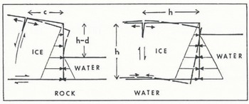
Fig. 11. A comparison between forward bending of an ice wall and upward arching of an ice shelf due to asymmetry between lithostatic pressure in ice and hydrostatic pressure in water at the calving front.
If the dependence between the calving ratio c/h and buoyancy ratio (ρw/ρI)d/h depicted in Figures 9 and 10 is correct, then calving slabs get relatively taller and thinner as water gets deeper prior to flotation of the slabs. If backward calving exceeds the forward velocity of a tide-water glacier, its calving ice wall retreats, often into deeper water if the glacier occupies a foredeepened fiord. Hence, c/h will be reduced and, if the section of the glacier weakened by transverse crevasses, as depicted in Figure 8, becomes afloat, tabular calving for which c/h ≈ 1 becomes possible in addition to slab calving for which c/h << 1. However, tabular icebergs released from this floating section of the glacier will be weakened at intervals where shear rupture in vertically bending shear bands allowed transverse crevasses to open. Flexural arching can therefore be accommodated by shear in these shear bands, as depicted in Figure 12. Since ice slabs are only weakly held together across these shear bands, the tabular iceberg may disintegrate by slab calving even while it is being released from the floating ice front. Reference EpprechtEpprecht (1987) described this disintegration for blocks H, J and K, tabular icebergs released from the north side of Jakobshavns Isbrae (69° 10′ N, 50° 10′ W) in Greenland. Since c/h ≈ 1 for these blocks, they began to rotate as they detached from the ice front: “During the rotation of block H, more crevasses opened in the newly separated section of the glacier and, as a result, blocks J and Κ became more free (Fig. 4). These then fell over, one after the other, like falling dominoes.... Within 7 min, not only did the part which had become separated from the glacier by the main fissure disintegrate into blocks, but these blocks had also toppled over. Afterwards, they all lay as large white slabs, several hundred meters across, closely packed together in the fjord (Fig. 2). Their surfaces were relatively smooth and very clean.” The calving section of Jakobshavns Isbne is shown in Figure 13. It consists of ice walls at the north and south sides that become an ice shelf in the center as water deepens along the calving front.

Fig. 12. A comparison between forward bending of an ice wall and upward arching of an ice shelf due to shear displacements between ice slabs. Top: behind the ice wall, τs = σxx = 0 across crevasses. Widening of the crevasses is due to increasing forward bending of ice slabs between crevasses, so that extending flow at the ice surface is caused by bending stress τs within each slab, not by σxx within slabs, and this produces an increasing surface slope (dashed line). Bottom: in the ice shelf, upward arching is caused by shear within shear bands that close after the glacier becomes afloat. This shear relieves forward bending (dashed line) caused by σxx that is tensile on the top surface and compressive on the bottom surface, as shown in Figure 11.

Fig. 13. Calving from Jakobshavns Isbræ, Greenland (orthophotograph by KUCERA International, Inc., with elevation contours in meters based on photogrammetri; measurements by H. Brecher).
Conclusions
A possible decrease in claving ratio c/h with increasing water depth (Figs 9 and 10), forward bending and upward arching both related to shear bands (Fig. 12) and the calving description by Reference EpprechtEpprecht (1987) for Jakobshavns Isbne (Fig. 13) raise the possibility that Equations (34) may be a general calving law that has broad applications to all calving glaciers. In a private letter, A. Post (21 June 1990) stated that he recognized four kinds of calving from Alaskan tide-water glaciers. All four may be represented in USGS photograph number 87V2–058 of Miles Glacier, supplied by Post and reproduced here as Figure 14:
-
1. Normal slab calving. The ice wall stands on dry land (d = 0) or in shallow water (d << h) and may be frozen to the bed. In this case, on Deception Island, α ≈ 0.3 near the ice wall due to bending shear and α ≈ 0.06 further upslope due to bed traction (Reference HughesHughes, 1989). Slabs the height of the ice wall, some tens of meters wide, and under 10 m thick calve at irregular intervals. Normal slab calving seems to be active on the photograph left side of the calving front of Miles Glacier. Post called this “steady-state” calving.
-
2. Unstable recessional calving. The calving rate exceeds the ice velocity, causing an ice wall standing in water to retreat on a bed that slopes downward inland, thereby reducing the lithostatic overburden of ice on the bed
. This increases h and reduces α near the ice wall in positive feed-back, so that normal slab calving is replaced by accelerated calving of thinner slabs that may create a calving bay if the calved slabs can be evacuated faster than the calving rate. Unstable recessional calving seems to be active on the photograph right side of the calving front of Miles Glacier. Post said a “retracted stable position” would re-establish normal slab calving at or near the head of tide water if the downsloping bed sloped upward further inland.
-
3. Sudden tabular calving. A large tabular section of the glacier suddenly and uniformly becomes uncoupled from the bed, probably due to a build-up of basal hydrostatic pressure to the flotation pressure (d = hρI/ρw). The large transverse rift at the rear of the calving section on the photograph right side of Miles Glacier could have released this section as a single tabular iceberg if Miles Glacier had been floating. Post described these calving events as being virtually identical to the calving of tabular icebergs from the floating front of Jakobshavns Isbrae. If the planar dimensions of the tabular section exceed its thickness, a tabular iceberg moves away from the ice front intact. Otherwise, it rears up on one side, rolls over and disintegrates completely within minutes.
-
4. Frequent buoyancy calving. Large sections of the ice front calve frequently when they become fully buoyant (d < hρI/ρw), while other grounded sections remain intact (d > hρI/ρw). These two conditions seem to apply to the photograph right side and the photograph left side, respectively, of Miles Glacier. For other tide-water glaciers, Post observed this calving process when the calving front is retreating into water up to 400 m or more in depth, and it seems to be the dominant form of calving from Columbia Glacier during the current rapid retreat. However, water in front of Miles Glacier is not this deep.

Fig. 14. Calving from Miles Glacier, Alaska (U.S.G.S. photograph 87V2–058, supplied by A. Post).
All of these four kinds of calving might be accommodated by the bending-shear mechanism quantified in Equations (34). The variables in this equation, h, d, c and θ, with α ≈ θ at the calving front, determine the calving velocity uc . They have been observed by Post to be important, and they seem to have at least the correct qualitative relationships to observed calving rates. Data are insufficient to determine whether Equations (34) is a reliable quantitative expression for calving rates along the great variety of calving fronts provided by Jakobshavns Isbrae. However, it is clear that calving events are associated with new crevasses along the calving front and within one or two ice thicknesses behind the calving front that have no apparent relationship to older crevasses formed far upstream and carried passively to the calving front (unpublished photogrammetric measurements by P. Prescott). This argues in favor of a local calving mechanism linked to the bending force and the bending moment at the calving front.
Some obvious features of this analysis should be emphasized. First, ablation at the ice wall is ignored. Ablation melts back the ice wall during bending shear, so the ice wall does not lean forward as much as it bends forward and may even lean backward. Ablation reduces s in Equations (25), and θ in Equations (26) is the forward bending angle of the opening crevasse, not of the ice wall (see Fig. 6). Secondly, the ice wall is on a flat bed, so extending flow due to ice riding up on to a terminal moraine is not considered. Instead, extending flow is caused by σ xx in Equations (14) prior to shear bands becoming transverse crevasses, and by bending creep causing transverse crevasses to widen toward the calving ice wall (see Fig. 12, top). Thirdly, steepening of surface slope α toward the calving ice wall is primarily due to the widening of transverse crevasses by increasing bending creep (see Fig. 12, top), and this increase of α increases the forward ice velocity and the backward calving rate. Fourthly, downward calving of ice slabs requires either crushing or ablating ice at the base of the ice wall. However, these mechanisms do not control the calving rate; see Reference Hughes and NakagawaHughes and Nakagawa (1989). Fifthly, the calving rate given by Equations (34) is most reliable when the calving ratio c/h and viscoplastic exponent n are both small; ideally, c/h << 1 and n = 1. Since 0.1 < c/h < 0.4 is observed for ten tide-water glaciers and n = 3 for ice, Equations (34) only gives approximate calving rates. Use of Equations (34) is even more problematic, given the ambiguities in specifying ηv and θ Even so, it has a foundation in theory and in observation.
A less obvious constraint on the bending-creep calving mechanism is the time needed to form a shear band. In laboratory creep experiments, about 25 d were needed when τa was about 1 bar (Reference Hughes and NakagawaHughes and Nakagawa, 1989). This time constraint can be illustrated by calving from Columbia Glacier, for which uc = 7 m d−1, h = 160 m and c/h = 0.22, so that an ice slab having c = 35 m calves every 5d. This means that bending creep must begin about 210 m behind the calving front if a shear band is to fracture by shear rupture 35 m behind the calving front.
Acknowledgements
I thank A. Post for sharing his insights on calving from tide-water glaciers, R. Hooke for comments on an earlier version of this manuscript and P. Prescott for sharing his unpublished photogrammetric measurements of surface elevations, slopes, velocities and strain rates along the calving front of Jakobshavns Isbrae. This work was funded by U.S. National Science Foundation grant DPP-8400886 and Battelle, PNL, subcontract 017112-A-B1.
The accuracy of references in the text and in this list is the responsbility of the author, to whom queries should be addressed.


