


1. Introduction
Optimization over flow fields that satisfy equations governing fluid motion has many applications. While initially applied to computational aerodynamics (Mohammadi & Pironneau Reference Mohammadi and Pironneau2004), various situations ranging from sloshing of fluids in containers for transport (Ibrahim, Pilipchuk & Ikeda Reference Ibrahim, Pilipchuk and Ikeda2001; Terashima & Yano Reference Terashima and Yano2001) to the transport of a passive tracer for mixing (Eggl & Schmid Reference Eggl and Schmid2018), and from the flapping of a foil for propulsion and fluid energy conversion (Young, Lai & Platzer Reference Young, Lai and Platzer2014; Jones & Yamaleev Reference Jones and Yamaleev2015; Quinn, Lauder & Smits Reference Quinn, Lauder and Smits2015) to the optimal placement of an actuator (Passaggia & Ehrenstein Reference Passaggia and Ehrenstein2013; Economon, Palacios & Alonso Reference Economon, Palacios and Alonso2015; Pasche, Avellan & Gallaire Reference Pasche, Avellan and Gallaire2019), are all formulated as fluid mechanics problems coupled with optimization. For further industrial applications of computational fluid dynamical optimization, see Thévenin & Janiga (Reference Thévenin and Janiga2008). Fluid mechanical optimization also has applications beyond industrial engineering. For example, animal body actuation for propulsion in a fluid medium seeks to minimize the energetic cost of aerial (Berman & Wang Reference Berman and Wang2007; Pesavento & Wang Reference Pesavento and Wang2009; Vincent, Liu & Kanso Reference Vincent, Liu and Kanso2020) and aquatic (Pironneau & Katz Reference Pironneau and Katz1974; Kern & Koumoutsakos Reference Kern and Koumoutsakos2006; Tam & Hosoi Reference Tam and Hosoi2007; Michelin & Lauga Reference Michelin and Lauga2010, Reference Michelin and Lauga2011, Reference Michelin and Lauga2013; Tam & Hosoi Reference Tam and Hosoi2011; Eloy & Lauga Reference Eloy and Lauga2012; Alben, Miller & Peng Reference Alben, Miller and Peng2013; Montenegro-Johnson & Lauga Reference Montenegro-Johnson and Lauga2014; Was & Lauga Reference Was and Lauga2014; Maertens, Gao & Triantafyllou Reference Maertens, Gao and Triantafyllou2017) locomotion. Optimization is invoked in cardiovascular biomechanics (He et al. Reference He, Ghattas, Antaki and Dennis1994; Marsden Reference Marsden2014) and sports biomechanics such as rowing (Labbé et al. Reference Labbé, Boucher, Clanet and Benzaquen2019), where fluid dynamics is central to the mechanics. Optimization is also an important tool to study fundamental fluid dynamics. Fundamental bounds on fluid dynamics processes have arisen from the hypothesis that turbulence optimizes fluid mechanical transport (Doering & Constantin Reference Doering and Constantin1992, Reference Doering and Constantin1994; Nicodemus, Grossmann & Holthaus Reference Nicodemus, Grossmann and Holthaus1997a,Reference Nicodemus, Grossmann and Holthausb; Kerswell Reference Kerswell1998; Souza, Tobasco & Doering Reference Souza, Tobasco and Doering2020). And the perturbation that underlies the transition to turbulence bypassing a linear instability is also sought using fluid mechanical optimization (Pringle & Kerswell Reference Pringle and Kerswell2010; Pringle, Willis & Kerswell Reference Pringle, Willis and Kerswell2012; Kerswell, Pringle & Willis Reference Kerswell, Pringle and Willis2014). Much more insight into fundamental and applied problems could be derived had it not been for the difficulty of solving steady and time-dependent Navier–Stokes equations coupled with optimization.
Powerful optimization techniques have been developed in the low-Reynolds-number limit where viscous fluid forces dominate over inertial ones (Pironneau & Katz Reference Pironneau and Katz1974; Tam & Hosoi Reference Tam and Hosoi2007, Reference Tam and Hosoi2011; Eloy & Lauga Reference Eloy and Lauga2012; Michelin & Lauga Reference Michelin and Lauga2013; Montenegro-Johnson & Lauga Reference Montenegro-Johnson and Lauga2014; Was & Lauga Reference Was and Lauga2014). These techniques exploit cleverly the linearity and kinematic reversibility of the governing fluid equations at low Reynolds numbers to organize the optimization phase space (Shapere & Wilczek Reference Shapere and Wilczek1987; Avron, Gat & Kenneth Reference Avron, Gat and Kenneth2004). Furthermore, the linearity of the fluid dynamical equations also renders many of the low-Reynolds-number optimization problems convex, so the optimum is unique. The linearity and the time-reversibility of the governing equations do not hold when the Reynolds number associated with the flow is finite or large, and consequently the low-Reynolds-number techniques do not apply. In this regime, fundamental results are few and far between. No choice other than computation by brute force exists for making progress on fluid mechanical optimization problems. Modern computer hardware does allow for retaining the infinite-dimensional nature of optimization space (Thévenin & Janiga Reference Thévenin and Janiga2008; Pringle & Kerswell Reference Pringle and Kerswell2010; Pringle et al. Reference Pringle, Willis and Kerswell2012; Eggl & Schmid Reference Eggl and Schmid2018; Boujo, Fani & Gallaire Reference Boujo, Fani and Gallaire2019; Pasche et al. Reference Pasche, Avellan and Gallaire2019). Techniques based on the adjoint formulation that arise from using calculus of variations are used to derive gradients. Optimization is then carried out by modifying iteratively the optimization variables along the gradient, or a close variant thereof. However, the computational results of gradient-based methods from problems with nonlinear constraints have not been definitive because of the possibility of multiple local optima. An exhaustive computational search in the infinite-dimensional state space is impossible, and consequently whether the global optimum was found has remained unknown.
This article has two objectives. The first is to pose the fluid mechanical brachistochrone problem and solve one of its instances. The problem asks for the shortest time to move an object in a fluid a fixed distance within a limited work budget. The problem is inspired by the brachistochrone problem introduced by Johann Bernoulli, which is generally considered to have kick-started the calculus of variations (Goldstine Reference Goldstine2012). Compared to other extensions of Bernoulli's original formulation (e.g. Camassa et al. Reference Camassa, McLaughlin, Moore and Vaidya2008; Gurram et al. Reference Gurram, Raja, Mahapatra and Panchagnula2019), the motivation behind our formulation of the fluid mechanical brachistochrone differs. Ours is designed to epitomize high-Reynolds-number kinematic optimization and highlight the essential difficulties introduced by fluid dynamic nonlinearities. The salient characteristics of solutions to simple problems such as this one can be used as building blocks to rationalize kinematic optimization results in more complex problems such as biolocomotion. The second objective of this article is to demonstrate that the local optimum found by adjoint-based numerical algorithms is globally optimal. We present a computational test for this purpose. Such a test for fluid mechanical optimization problems in the high-Reynolds-number case is constructed by exploiting the quadratic nature of the nonlinearity in the governing fluid equations. A positive conclusion on this test establishes that the computed local optimum also constitutes a bound on the objective function, and therefore must be global.
The solution to the fluid mechanical brachistochrone in its full generality depends on the shape of the object. Here, we seek to illustrate the essential features of the solution for a streamlined body, where hydrodynamic drag is caused predominantly by skin friction. With this in mind, we consider the case of a flat plate moving parallel to its surface. Non-trivial flow occurs in a thin boundary layer near the plate and in its wake, which is modelled by the Prandtl boundary layer equations. These equations retain the inertia of the fluid, thus violating linearity and kinematic reversibility. No convexity results are known for this case of the optimization problem, especially when the Reynolds number is large, thus any computed local minimum need not be global.
The problem is equivalent to determining the profile of transient speed  $V({\tilde {{t}}})$ with time
  ${\tilde {{t}}}$ of a flat plate of length
  $L$ moving parallel to its surface a distance
  $D$ in time
  $T$ (see figure 1) that minimizes the mechanical work
  ${\tilde {{\mathcal {W}}}}$. The surrounding fluid of density
  $\rho$ and viscosity
  $\mu$ (with
  $\nu = \mu /\rho$) is of infinite extent and initially static, and the flow is considered laminar. The plate is infinitesimal in its thickness and infinitely long in the third dimension so that the resulting flow is two-dimensional and confined to a thin layer close to the plate.

Figure 1. Schematic of a flat plate moving through a fluid.
The dimensionless parameters  $\textit {Re} = \rho DL/(\mu T)$ and
  $\epsilon = D/L$ represent the Reynolds number and the target distance to be travelled relative to the plate length. We consider the regime for
  $\textit {Re} \gg 1$ and arbitrary
  $\epsilon$, thereby retaining the essential nonlinearity in the governing equations. This is in contrast to the case
  $\epsilon \ll 1$ considered by Mandre (Reference Mandre2020), which eliminates the nonlinearity and, in return, facilitates an analytical solution. Here we use a gradient-descent method based on calculus of variations for numerical optimization, where an adjoint formulation is used to calculate the gradient. The details of the adjoint-based gradient descent and characterization of the optimum kinematics are presented in § 3. We find that for
  $\epsilon \gg 1$, the minimum work
  $\tilde {\mathcal {W}}_{min}$ needed for travel in fixed duration
  $T$, or equivalently the shortest time
  $T_{min}$ under a work budget
  $\tilde {\mathcal {W}}$, approach asymptotically
 \begin{equation} {\tilde{{\mathcal{W}}}}_{min} \approx 1.328 \sqrt{\dfrac{\mu \rho D^5L}{T^3}}, \quad T_{min} \approx 1.21 \left(\dfrac{\mu \rho D^5 L}{{\tilde{{\mathcal{W}}}}^2}\right)^{1/3}. \end{equation}
The result in (1.1a,b) also suffers from the possibility that the local minimum found is not a global one. To confirm its global nature, we derive a sufficient condition for global optimality and apply it computationally. We start in § 2 with the derivation of this condition, which applies to optimization of quadratic objectives constrained by quadratic partial differential equations. This addresses a major criticism of gradient-based optimization methods, not only for fluid mechanical optimization but also generally for quadratic programming problems. The condition uses the Lagrange dual formulation to derive a bound on the objective function that agrees with the calculated optimum. The condition is then used in § 3 to demonstrate computationally that the optimum found for the brachistochrone problem is global.
2. Spectral condition for global optimality
Consider a time-independent region  $\varOmega$ occupied by a fluid for a time
  $t\in [0,T]$. The objective is to find
 $$\begin{gather} \mathcal{W}_{min} = \min_{\boldsymbol{u}(\boldsymbol{x},t)} \mathcal{W}[\boldsymbol{u}] \equiv \int_0^T \int_\varOmega (q(\boldsymbol{u})+l(\boldsymbol{u}))\,\mathrm{d} \varOmega\,\mathrm{d} t \end{gather}$$
 $$\begin{gather}\text{subject to} \quad \boldsymbol{u}_t + \boldsymbol{Q}(\boldsymbol{u}) + \boldsymbol{L}(\boldsymbol{u}) + \boldsymbol{C} = 0, \end{gather}$$
for  $\boldsymbol {x} \in \varOmega$ and
  $t\in (0,T)$, where
  $q(\boldsymbol {u})$ and
  $\boldsymbol {Q}(\boldsymbol {u})$ are quadratic,
  $l(\boldsymbol {u})$ and
  $\boldsymbol {L}(\boldsymbol {u})$ are linear, and
  $\boldsymbol {C}$ is constant in
  $\boldsymbol {u}$ and its spatial derivatives. In particular, assume that
  $q(\boldsymbol {u})$ and
  $\boldsymbol {Q}(\boldsymbol {u})$ do not depend on
  $\boldsymbol {u}_t$ (here, subscript
  $t$ denotes differentiation with respect to
  $t$). The optimization may be over the initial condition for
  $\boldsymbol {u}$ (e.g. finding the minimal seed for transition to turbulence – see Pringle & Kerswell Reference Pringle and Kerswell2010; Pringle et al. Reference Pringle, Willis and Kerswell2012), the boundary condition for
  $\boldsymbol {u}$ (e.g. kinematic optimization – see Eggl & Schmid Reference Eggl and Schmid2018; Boujo et al. Reference Boujo, Fani and Gallaire2019; Mandre Reference Mandre2020), the forcing
  $\boldsymbol {C}$ (e.g. see Pasche et al. Reference Pasche, Avellan and Gallaire2019), or any combination of the above.
The optimization proceeds by writing the Lagrangian
 \begin{equation} \mathcal{L}[\boldsymbol{u}, \boldsymbol{\alpha}] = \int_0^T \int_\varOmega \left[ q + l - \boldsymbol{\alpha}\boldsymbol{\cdot} (\boldsymbol{u}_t + \boldsymbol{Q} + \boldsymbol{L} + \boldsymbol{C}) \right]\mathrm{d} \varOmega\,\mathrm{d} t, \end{equation}
where  $\boldsymbol {\alpha }(\boldsymbol {x}, t)$ is the adjoint field. Accounts of how to find the adjoint and the gradients
  $\delta \mathcal {L}/\delta \boldsymbol {u}$, and descend along it, can be found elsewhere (e.g. He et al. Reference He, Ghattas, Antaki and Dennis1994; Mohammadi & Pironneau Reference Mohammadi and Pironneau2004; Pringle & Kerswell Reference Pringle and Kerswell2010; Pringle et al. Reference Pringle, Willis and Kerswell2012; Passaggia & Ehrenstein Reference Passaggia and Ehrenstein2013). Suppose that this process converges to
  $\boldsymbol {u}=\boldsymbol {u}_*$, corresponding to
  $\boldsymbol {\alpha } = \boldsymbol {\alpha }_*$ and
  $\mathcal {W} = \mathcal {W}_*$.
To test if the converged state is a global minimum, we construct the Lagrange dual  $\mathcal {D}[\boldsymbol {\alpha }] = \inf _{\boldsymbol {u}} \mathcal {L}[\boldsymbol {u}, \boldsymbol {\alpha }]$. The value of
  $\mathcal {D}[\boldsymbol {\alpha }]$ for any
  $\boldsymbol {\alpha }$ is a lower bound on
  $\mathcal {W}[\boldsymbol {u}]$ for
  $\boldsymbol {u}$ that satisfies (2.1b) (Boyd & Vandenberghe Reference Boyd and Vandenberghe2004). The proof for (2.2) is as follows:
 \begin{equation} \mathcal{W}[\boldsymbol{u}] = \mathcal{L}[\boldsymbol{u},\boldsymbol{\alpha}] \geqslant \mathcal{D}[\boldsymbol{\alpha}], \end{equation}
where in the first equality, we use that  $\boldsymbol {u}$ satisfies (2.1b), and in the following inequality, we use the infimum property of
  $\mathcal {D}$.
For the spectral condition, we choose  $\boldsymbol {\alpha } = \boldsymbol {\alpha }_*$ to evaluate the bound. To determine
  $\mathcal {D}[\boldsymbol {\alpha }_*]$, we need to minimize
  $\mathcal {L}[\boldsymbol {u}, \boldsymbol {\alpha }_*]$ over all
  $\boldsymbol {u}$, which is where the quadratic nature of the functionals is instrumental. Since both
  $\mathcal {W}$ and (2.1b) are quadratic in
  $\boldsymbol {u}$, the first variation conditions in
  $\boldsymbol {u}$ are linear in
  $\boldsymbol {u}$ and identical to the adjoint equations employed during the gradient descent. Thus they are satisfied automatically by
  $\boldsymbol {u}_*$. But the satisfaction of the first variation condition does not guarantee that
  $\boldsymbol {u}_*$ is a minimizer. The total nonlinear variation of
  $\mathcal {H}[\boldsymbol {u}, \boldsymbol {\alpha }_*] = \mathcal {L}[\boldsymbol {u}, \boldsymbol {\alpha }_*] - \mathcal {L}[\boldsymbol {u}_*, \boldsymbol {\alpha }_*]$ determines whether
  $\boldsymbol {u}_*$ is the minimizer of
  $\mathcal {L}[\boldsymbol {u}, \boldsymbol {\alpha }_*]$. If the variation around the computed minimum can be proven to be positive semi-definite, then the bounding property of the Lagrange dual implies that the minimum is global. However, proving the positive semi-definiteness of a general functional is difficult. Here, because of the quadratic nature of the functional, its positive semi-definiteness can be tested by solving a linear eigenvalue problem. This quadratic functional for the second variation of
  $\mathcal {L}$ is
 \begin{equation} \mathcal{H}[\boldsymbol{u}, \boldsymbol{\alpha}_*] = \int_0^T \int_\varOmega (q - \boldsymbol{\alpha}_*\boldsymbol{\cdot} \boldsymbol{Q})\,\mathrm{d}\varOmega\,\mathrm{d} t. \end{equation}
If  $\mathcal {H}[\boldsymbol {u}, \boldsymbol {\alpha }_*]$ is positive semi-definite in
  $\boldsymbol {u}$, then
  $\boldsymbol {u}_*$ is the minimizer of
  $\mathcal {L}[\boldsymbol {u},\boldsymbol {\alpha }_*]$, and
  $\mathcal {W}_*$ is its minimum. Instead, if
  $\mathcal {H}[\boldsymbol {u}, \boldsymbol {\alpha }_*]$ is not positive semi-definite in
  $\boldsymbol {u}$, then the minimum
  $D[\boldsymbol {\alpha }_*]$ is
  $-\infty$. Mathematically,
 \begin{equation} \mathcal{D}[\boldsymbol{\alpha}_*] = \begin{cases} \mathcal{W}_*, & \text{if } \mathcal{H}[\boldsymbol{u}, \boldsymbol{\alpha}_*] \geqslant 0 \text{ for all } \boldsymbol{u}, \\ -\infty, & \text{otherwise.} \end{cases} \end{equation}
Since  $\boldsymbol {u}_t$ does not appear in the integrand for
  $\mathcal {H}$, the second variation is positive semi-definite if and only if
 \begin{equation} \int_\varOmega (q - \boldsymbol{\alpha}_*\boldsymbol{\cdot} \boldsymbol{Q})\,\mathrm{d}\varOmega \geqslant 0\quad \text{for all } \boldsymbol{u} \text{ and every } t. \end{equation}
 To summarize, if (2.6) is satisfied, then  $\mathcal {W}_*$ is a lower bound on
  $\mathcal {W}[\boldsymbol {u}]$ that is attained at
  $\boldsymbol {u}_*$, and is therefore the global minimum. Failure to satisfy (2.6) does not necessarily mean that
  $\boldsymbol {u}_*$ is not global but could imply a duality gap (Boyd & Vandenberghe Reference Boyd and Vandenberghe2004). Duality gap is defined as the smallest possible difference
  $\mathcal {W}[\boldsymbol {u}] - \mathcal {D}[\boldsymbol {\alpha }]$ for
  $\boldsymbol {u}$ satisfying constraints (2.1b). The duality gap is non-negative by definition and measures the tightness of the bound offered by the Lagrange dual. The presence or absence of a duality gap for general optimization problems is difficult to predict a priori. However, satisfaction of the spectral condition demonstrates both the absence of a finite duality gap and the attainment of a global minimum.
As an example, if (2.1b) represents the incompressible Navier–Stokes equations, then  $\boldsymbol {u}$ is the divergence-free velocity field,
  $\boldsymbol {Q}=\boldsymbol {u} \boldsymbol {\cdot }\boldsymbol {\nabla }\boldsymbol {u} + \boldsymbol {\nabla } p$ represents the advection term (where
  $\boldsymbol {\nabla } p$ ensures that
  $\boldsymbol {Q}$ is divergence-free),
  $\boldsymbol {L} = -\nu \nabla ^2 \boldsymbol {u}$ represents the viscous term, and
  $\boldsymbol {C}$ the body force term. For objectives such as the dissipation rate,
  $q(\boldsymbol {u}) = |\boldsymbol {\nabla }\boldsymbol {u}|^2$ and
  $l(\boldsymbol {u})=0$, the assumptions that the nonlinearities be quadratic and independent of
  $\boldsymbol {u}_t$ are satisfied. The corresponding condition for global optimality is
 \begin{equation} \int_\varOmega ( |\boldsymbol{\nabla}\boldsymbol{u}|^2 - \boldsymbol{\alpha}_* \boldsymbol{\cdot}(\boldsymbol{u}\boldsymbol{\cdot}\boldsymbol{\nabla}) \boldsymbol{u} )\mathrm{d}\varOmega \geqslant 0, \end{equation}
over all divergence-free  $\boldsymbol {u}$, applied separately at each
  $t$. A condition equivalent to (2.7) was derived by Doering & Constantin (Reference Doering and Constantin1994) in the context of the background method for turbulent transport. They named it the ‘spectral constraint’ because it requires that the self-adjoint linear operator underlying the quadratic form, i.e. the Hessian of
  $\mathcal {L}[\boldsymbol {u},\boldsymbol {\alpha }_*]$, has non-negative eigenvalues. The interpretation of the background method in terms of a Lagrange dual formulation was presented by Kerswell (Reference Kerswell1999), with which this derivation shares much similarity. Based on this nomenclature, we term (2.6) the spectral condition.
3. Work-minimizing kinematics of a flat-plate
We now turn our attention to minimizing the work done to move a flat plate.
3.1. Mathematical formulation
In the limit  $\textit {Re} \gg 1$, the problem is formulated based on a thin viscous boundary layer that governs the drag. The fluid outside this layer, to leading order in
  $\textit {Re}$, remains stationary as the plate moves. To model the flow in the boundary layer, we use a coordinate system attached to the leading edge of the plate, as shown in figure 1, and a reference frame attached to far field stationary fluid. The coordinates
  ${\tilde {{x}}}$,
  ${\tilde {{y}}}$ attached to the plate, and the boundary layer flow velocity
  $({\tilde {{u}}}({\tilde {{x}}},{\tilde {{y}}},{\tilde {{t}}}), {\tilde {{v}}}({\tilde {{x}}},{\tilde {{y}}},{\tilde {{t}}}))$ in a reference frame of the far field fluid, satisfy the Prandtl equations
 $$\begin{gather} {\tilde{{u}}}_{\tilde{{t}}} + ({\tilde{{u}}}+V) {\tilde{{u}}}_{\tilde{{x}}} + {\tilde{{v}}} {\tilde{{u}}}_{\tilde{{y}}} - \nu {\tilde{{u}}}_{{\tilde{{y}}}{\tilde{{y}}}} = 0, \end{gather}$$
 $$\begin{gather}{\tilde{{u}}}_{\tilde{{x}}} + {\tilde{{v}}}_{\tilde{{y}}} = 0, \end{gather}$$
where subscripts  ${\tilde {{x}}}$,
  ${\tilde {{y}}}$ and
  ${\tilde {{t}}}$ denote partial differentiation with respect to that variable. The essential nonlinearity in fluid dynamics governing equations is due to the advection, which is retained in this formulation. Exploiting the reflection symmetry, we consider only the flow field for
  ${\tilde {{y}}}\geqslant 0$ and the drag on one face of the plate. These equations are subject to the boundary conditions
 $$\begin{gather} {\tilde{{u}}}(0\leqslant {\tilde{{x}}}\leqslant L, {\tilde{{y}}}, {\tilde{{t}}}) + V (t) = 0, \end{gather}$$
 $$\begin{gather}{\tilde{{u}}}_{\tilde{{y}}}({\tilde{{x}}}<0 \text{ or } {\tilde{{x}}}>L, {\tilde{{y}}}, {\tilde{{t}}}) = 0, \end{gather}$$
 $$\begin{gather}{\tilde{{u}}}({\tilde{{x}}}, {\tilde{{y}}}\to \infty, {\tilde{{t}}}) = 0, \end{gather}$$
 $$\begin{gather}{\tilde{{u}}}({\tilde{{x}}}\to -\infty, {\tilde{{y}}}, {\tilde{{t}}}) = 0, \end{gather}$$
 $$\begin{gather}{\tilde{{u}}}({\tilde{{x}}},{\tilde{{y}}},{\tilde{{t}}}=0) = 0. \end{gather}$$
The drag force is given by  ${\tilde {{f}}} = 2 \int _0^L\mu \, {\tilde {{u}}}_{\tilde {{y}}}({\tilde {{x}}},{\tilde {{y}}}=0,{\tilde {{t}}})\,{\rm d}\kern0.7pt {\tilde {{x}}}$, and the net work done for the motion is
 \begin{equation} {\tilde{{\mathcal{W}}}} = \int_0^t V(t) \int_0^l 2 \mu\, {\tilde{{u}}}_{\tilde{{y}}}({\tilde{{x}}},{\tilde{{y}}}=0,{\tilde{{t}}})\,{\rm d}{\tilde{{x}}}\,{\rm d}{\tilde{{t}}}. \end{equation}
The variables are rescaled as
 \begin{equation} {\tilde{{t}}} = Tt,\quad {\tilde{{x}}} = Lx,\quad {\tilde{{y}}} = \delta y,\quad {\tilde{{u}}} = \dfrac{D}{T}\,u, \quad {\tilde{{v}}} = \dfrac{D\delta}{TL}\,v, \end{equation}
where  $\delta = \sqrt {\nu T}$, to yield the dimensionless form of the governing boundary layer equations as
 $$\begin{gather} \mathcal{M} \equiv u_t + \epsilon (u+f)u_x + \epsilon v u_y - u_{yy} = 0, \end{gather}$$
 $$\begin{gather}\mathcal{C} \equiv u_x + v_y = 0, \end{gather}$$
in the semi-infinite half-space  $y\geqslant 0$, and
 $$\begin{gather} u|_{x\in P, y=0} + f(t) = u_y|_{x \not\in P, y=0} = 0, \end{gather}$$
 $$\begin{gather}v|_{y=0} = u_y|_{y=\infty} = u|_{x={\pm}\infty} = u|_{t=0} = 0, \end{gather}$$
where  $P = [0,1]$ specifies the extent of the flat plate, and
  $f(t) = (T/D)\,V({\tilde {{t}}})$ is the dimensionless plate speed. Subscripts
  $x$,
$x$,  $y$ and
  $t$ on
  $u$ and
  $v$ denote partial derivatives.
The following notation will be also used
 \begin{equation} \langle \phi \rangle_{\gamma_1 \dots \gamma_m} \equiv \iiint \phi\,\mathrm{d} \gamma_1 \dots \mathrm{d} \gamma_m, \end{equation}
where  $\gamma _i$ could be any of
  $x$,
$x$,  $y$ or
  $t$. The limits of integration are
  $[0,1]$ on
  $t$,
$t$,  $[0,\infty ]$ on
  $y$, and
  $[-\infty, \infty ]$ on
  $x$. For example,
  $\langle \phi \rangle _{xy}$ is
  $\int _0^\infty \int _{-\infty }^\infty \phi \,\mathrm {d}\kern0.7pt x \,\mathrm {d} y$. For simplicity,
  $\langle \phi \rangle \equiv \langle \phi \rangle _{xyt}$.
The work done is  ${\tilde {{\mathcal {W}}}} = 2D^2 L \sqrt {{\mu \rho }/{T^3}}\ \mathcal {W}[f]$, where
  $\mathcal {W}[f] = \langle f(t)\,u_y(x,y=0,t)\rangle _{xt}$. For
  $(u,v)$ satisfying (3.5) and (3.6), the work done must appear as an increase in the kinetic energy of the fluid or be viscously dissipated, i.e.
 \begin{equation} \mathcal{W}[f] = \hat{\mathcal{W}}[f] \equiv \left\langle\left. \tfrac{1}{2} u^2\right|_{t=1} \right\rangle_{xy} + \langle u_y^2 \rangle, \end{equation}
which is necessarily positive.
The objective of the optimization is to minimize  $\mathcal {W}[f]$ subject to
  $\mathcal {M} = \mathcal {C}= 0$ in the fluid. The Lagrangians using
  $\mathcal {W}[f]$ and
  $\hat {\mathcal {W}}[f]$ are
 \begin{equation} \mathcal{L} = \mathcal{W}[f] - \langle \alpha \mathcal{M} + \epsilon \beta \mathcal{C} \rangle - \lambda \mathcal{D} \end{equation}
and
 \begin{equation} \hat{\mathcal{L}} = \hat{\mathcal{W}}[f] - \langle \hat{\alpha} \mathcal{M} + \epsilon \beta \mathcal{C} \rangle - \lambda \mathcal{D}, \end{equation}
respectively, where  $\alpha (x,y,t)$,
  $\hat {\alpha }(x,y,t)$,
  $\beta (x,y,t)$ and
  $\lambda$ are Lagrange multipliers, and
 \begin{equation} \mathcal{D} = \langle f \rangle_t - 1 \end{equation}
is the constraint on the distance travelled by the plate. We also define  $\hat {u} = u + f$, which is the
  $x$-component of the fluid velocity in the reference frame of the plate. Gradient descent is convenient using
  $\mathcal {L}$ because in these variables, the adjoint satisfies an equation similar to that for
  $u$. On the other hand, the spectral condition is derived using
  $\hat {\mathcal {L}}$, which when expressed in
  $\hat {u}$ reveals an eigenvalue problem with homogeneous boundary conditions. By virtue of (3.8), the two formulations in
  $\mathcal {L}$ and
  $\hat {\mathcal {L}}$ are equivalent, related by
  $\hat {\alpha } = \alpha + u$.
The multipliers  $\alpha$ and
  $\beta$ satisfy the condition that first variations of
  $\mathcal {L}$ due to
  $u$ and
  $v$ vanish, i.e.
 $$\begin{gather} \alpha_t + \epsilon (u+f) \alpha_x + \epsilon (v\alpha)_y + \epsilon \beta_x + \alpha_{yy} = 0, \end{gather}$$
 $$\begin{gather}\beta_y = \alpha u_y, \end{gather}$$
in  $y>0$, subject to the boundary conditions
 $$\begin{gather} \alpha|_{x \in P, y=0} - f (t) = \alpha_y|_{x \not\in P, y=0} = 0, \end{gather}$$
 $$\begin{gather}\beta|_{y=\infty} = \alpha_y|_{y=\infty} = \alpha|_{x=\infty} = \alpha|_{t=1} = 0. \end{gather}$$
 The first variation with respect to  $f$, given by
 \begin{equation} \dfrac{\delta \mathcal{L}}{\delta f} = \left\langle \left[u_y - \alpha_y\right]_{y=0} \right\rangle_x - \epsilon \langle \alpha u_x \rangle_{xy} - \lambda, \end{equation}
must also vanish.
The optimization is carried out using gradient descent in  $f$ using (3.13) while solving (3.5), (3.6), (3.11) and (3.12) numerically, as described in Appendix A. We find that this procedure converges to
  $f=f_*$,
  $u=u_*$,
  $v=v_*$,
  $\alpha = \alpha _*$ and
  $\mathcal {W}[f]=\mathcal {W}_{min}$, as
  $\delta \mathcal {L}/\delta f$ approaches 0. The converged profiles for
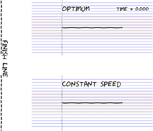
  $f(t)$ are shown in figure 2, and the corresponding
  $\mathcal {W}_{min}$ in figure 3(a).

Figure 2. Optimal  $f(t)$ for different
  $\epsilon$ coded according to the colour in the adjoining colourbar. The dotted curve shows
  $f_0(t)$ from (3.19a), and the dashed curve shows unity.

Figure 3. Minimum work for translating a flat plate and the verification of the corresponding spectral constraint. (a) Plot of  $\mathcal {W}_{min}$ as a function of
  $\epsilon$. The dotted line shows
  $\mathcal {W}_{0,min}\approx 1.014$ from (3.19b), and the dashed line shows
  $0.664 \epsilon ^{1/2}$. (b) Minimum
  $\lambda _{min} = \min _{t\in (0,1)} \lambda (t)$ (blue circles) and maximum
  $\lambda _{max} = \max _{t\in (0,1)} \lambda (t)$ (red squares) of
  $\lambda (t)$. Thus the region shaded grey shows the values taken by
  $\lambda (t)$ for the corresponding
  $\epsilon$. By virtue of (3.18), the second variation (3.17) is given by
  $\lambda \langle \psi ^2 + \psi _x^2 + \psi _y^2 \rangle$. Since the quantity in the angled brackets is positive definite,
  $\lambda (t)$ being positive for all
  $t$ implies that the second variation in (3.17) is also positive definite, thus the spectral condition is satisfied.
3.2. Spectral condition
To prove that the computed minimum is global, we choose  $\hat {\alpha }=\hat {\alpha }_* = \alpha _* + u_*$ and the Lagrange dual
 \begin{equation} \mathcal{D}[\hat{\alpha}] \equiv \min_{u,v,\beta,f} \hat{\mathcal{L}}. \end{equation}
Because  $\hat {\mathcal {L}}$ is quadratic in
  $(u,v,\beta,f)$, by virtue of (3.11) and (3.12)
  $(u_*,v_*, \beta _*,f_*)$ is a stationary point of
  $\hat {\mathcal {L}}$ in those variables, for which
  $\hat {\mathcal {L}} = \mathcal {W}_{min}$. It is the second variation
 \begin{equation} \mathcal{H}[\hat{\alpha}_*; u,v,f] = \hat{\mathcal{W}}[f] - \epsilon \left\langle \hat{\alpha}_* ((u+f)u_x + vu_y) \right\rangle \end{equation}
in  $(u,v,f)$ for
  $(u,v)$ satisfying (3.5b) that determines whether
  $(u_*,v_*, \beta _*,f_*)$ is a minimum of
  $\hat {\mathcal {L}}$. This leads to
 \begin{equation} \mathcal{W}[f] \geqslant \mathcal{D}[\hat{\alpha}_*] = \begin{cases} \mathcal{W}_{min}, & \text{if } \mathcal{H} \geqslant 0 \text{ for all } (u,v,f), \\ -\infty, & \text{otherwise}. \end{cases} \end{equation}
The condition  $\mathcal {H} \geqslant 0$ is satisfied if for each
  $t\in (0,1)$, we have
 \begin{equation} \varDelta[u,v] = \langle \hat u_y^2 -\hat{\alpha}_* \epsilon (\hat u \hat u_x + v \hat u_y) \rangle_{xy} \geqslant 0, \end{equation}
for all  $(\hat u,v)$ satisfying (3.5b) and (3.6).
Equation (3.5b) implies a stream function  $\psi$ such that
  $\hat {u} = \psi _y$ and
  $v = -\psi _x$. Substituting this in (3.17) and integrating by parts yields the related optimization problem
 \begin{equation} \left.\begin{gathered} \lambda(t) = \min_\psi \varDelta = \min_\psi \langle \psi_{yy}^2 +\epsilon \hat{\alpha}_{*x} \psi_y^2 - \epsilon \hat{\alpha}_{*y} \psi_x\psi_y \rangle_{xy}, \\ \text{subject to }\ \langle \psi^2 + \psi_x^2 + \psi_y^2 \rangle_{xy} = 1 \end{gathered}\right\} \end{equation}
for each  $t\in (0,1)$. The solution of (3.18) implies
  $\varDelta \geqslant \lambda (t)\,\langle \psi ^2 + \psi _x^2 + \psi _y^2 \rangle _{xy}$ and hence the spectral constraint is satisfied if
  $\lambda (t)\geqslant 0$ for
  $t\in (0,1)$. Here,
  $\lambda (t)$ is determined numerically by constructing the generalized eigenvalue problem from the linear operators underlying the quadratic forms in (3.18), which is described in Appendix A. As shown in figure 3(b),
  $\lambda (t)$ is positive for each
  $t$, thus proving that the local minimum found in § 3.1 is a global one.
3.3. Interpretation of the results
As seen in figures 2 and 3(a), the analytical solution by Mandre (Reference Mandre2020) derived for  $\epsilon \ll 1$,
 \begin{equation} f(t) = f_0(t) = C {t^{1/4} (1-t)^{1/4}} \end{equation}
and
 \begin{equation} \mathcal{W}_{min} = \mathcal{W}_{0,min} \approx 1.014, \end{equation}
where  $C \approx 1.62$, approximates the solution for finite
  $\epsilon \leqslant 0.5$. As
  $\epsilon$ increases beyond, the optimal
  $f(t)$ departs from
  $f_0(t)$, while
  $\mathcal {W}_{min}$ rises above
  $\mathcal {W}_{0,min}$. In particular,
  $f(t)$ starts from
  $f(0) = 0$ and ends at
  $f(1) = 0$ but flattens out in the middle. For
  $\epsilon \gtrsim 5$,
  $f(t)$ approaches unity, except at the start and the end. In other words, the optimum kinematics to cover a distance
  $D\gg L$ in time
  $T$ is to cruise at the average speed
  $U\approx D/T$, except to start and stop. For
  $\epsilon \gg 1$,
  $\mathcal {W}_{min}$ is also observed to rise
  $\propto \epsilon ^{1/2}$.
The following dimensional argument rationalizes these observations. The drag according to Blasius (Reference Blasius1907) for a flat plate moving at steady speed  $U$ is given by
  $0.664 \sqrt {\mu \rho U^3 L}$, and consequently, the work done to move the plate is
  ${\tilde {{\mathcal {W}}}}_\infty = 0.664 T \sqrt {\mu \rho U^5 L}$. Consider covering the distance
  $D=UT$ in two stages, of durations
  $aT$ and
  $(1-a)T$, moving with speeds
  $U_1 = bU/a$ and
  $U_2 = (1-b)U/(1-a)$, respectively, for constants
  $a$ and
  $b$ between 0 and 1. When
  $\epsilon \gg 1$, steady state is reached much faster than the duration of each segment, and the modified kinematics approximately incurs the work
 \begin{equation} 0.664 T \sqrt{\mu \rho U^5 L} \left(\dfrac{b^{5/2}}{a^{3/2}} + \dfrac{(1-b)^{5/2}}{(1-a)^{3/2}} \right). \end{equation}
This work is minimized when  $b=a$, or
  $U_1 = U_2 = U$. In other words, the penalty incurred in the work done when traveling fast outweighs the benefits accrued when traveling slower, explaining why the optimum avoids modulation of the speed. Converting
  ${\tilde {{\mathcal {W}}}}_\infty$ to a dimensionless form yields
  $\mathcal {W}_{min} \approx 0.664 \epsilon ^{1/2}$ for
  $\epsilon \gg 1$, agreeing up to leading order with the results of the computations as shown in figure 3(a). Accounting for the two sides of the plate leads to (1.1a,b).
It is seen readily why the optimal profile avoids an impulsive start and stop. For  $t\ll 1$ (and
  $1-t\ll 1$), owing to the development of the viscous boundary layer, the unsteady inertia
  $u_t$ and shear viscosity
  $u_{yy}$ in (3.5) dominate, while advection
 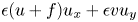 $\epsilon (u+f)u_x + \epsilon vu_y$ is negligible. Therefore, in the first variation condition (3.13), the dominant balance is between
  $u_y$ and
  $\alpha _y$. For an impulsive start, the initial shear stress profile on the plate is
  $u_y|_{y=0}\approx f(0)/\sqrt {{\rm \pi} t}$ due to the growth of the boundary layer thickness proportional to
  $\sqrt {t}$. The adjoint dynamics, due to their backwards evolution in time, does not ‘know’ about the impulsive start, and therefore cannot generate an
  $\alpha _y$ that matches this asymptotic behaviour. This behaviour can be observed explicitly in the analytical solution for
  $\epsilon \ll 1$ (Mandre Reference Mandre2020) and carries over to finite
  $\epsilon$. Therefore, for small
  $t$, one can always reduce the work done by eliminating any impulsive start (and analogously an impulsive stop).
We also find that for finite  $\epsilon$, the optimal starting and stopping dynamics behave proportionally to
  $t^{1/4}$ and
  $(1-t)^{1/4}$, respectively. This is observed in the numerical solution for over four orders of magnitude in
  $t$, as shown in figure 4. The reason is analogous to that in the analytical solution for vanishing
  $\epsilon$ in (3.19). Near the starting and stopping times, the advection is negligible and the optimal kinematics is governed by the viscous diffusion of momentum within the fluid, just as is the case when
  $\epsilon \ll 1$ (Mandre Reference Mandre2020), which causes this behaviour. To see this more clearly, consider the approximations of (3.5a) and (3.11a) for small
  $t$,
$t$,
 $$\begin{gather} u_t - u_{yy} \approx 0, \end{gather}$$
 $$\begin{gather}\alpha_t + \alpha_{yy} \approx 0, \end{gather}$$
driven by the boundary conditions  $u|_{y=0} = -f(t)$ and
  $\alpha |_{y=0} = f(t)$. The approximate gradient for small
  $t$ is dominated by
 \begin{equation} \dfrac{\delta \mathcal{L}}{\delta f} \approx \left\langle \left[u_y - \alpha_y\right]_{y=0} \right\rangle_x. \end{equation}
The first term in this expression is the part of the variation arising from a change in  $f(t)$, while the second term arises from the resulting variation in the shear force on the plate. Because
  $x$ derivatives drop out of this approximation, the solution to (3.21) is uniform in
  $x$, and the integral in
  $x$ can be dropped. Elimination of an impulsive start implies a power-law behaviour for
  $f$ at small
  $t$, say
  $f(t) \approx a t^n$ for
  $0< t<\hat {t}$, where
  $\hat {t} \gg t$ is a time until which the approximation remains valid. The Dirichlet-to-Neumann map for the heat equation (3.21) then implies
 $$\begin{gather} u_y|_{y=0} \approx{-}\int_0^t \dfrac{a n s^{n-1}}{\sqrt{{\rm \pi}(t-s)}}\,\mathrm{d} s ={-} \dfrac{a n t^{n-1/2}}{\sqrt{\rm \pi}} \int_0^1 \dfrac{w^{n-1}}{\sqrt{1-w}}\,\mathrm{d} w, \end{gather}$$
 $$\begin{gather}\alpha_y|_{y=0} \approx{-}\int_t^{\hat{t}} \dfrac{a n s^{n-1}}{\sqrt{{\rm \pi}(s-t)}}\, \mathrm{d} s ={-}\dfrac{a n t^{n-1/2}}{\sqrt{\rm \pi}} \int_{t/\hat{t}}^1 \dfrac{1}{w^{n+1/2} \sqrt{1-w}}\,\mathrm{d} w, \end{gather}$$
where the second half of each equation is derived by using the transformation  $w=s/t$ for (3.23a) and
  $w=t/s$ for (3.23b). Substituting in (3.22) and using
  $t/\hat {t} \approx 0$ yields
 \begin{equation} \dfrac{\delta \mathcal{L}}{\delta f} \approx \dfrac{a n t^{n-1/2}}{\sqrt{\rm \pi}} \int_0^1 \dfrac{1}{\sqrt{1-w}} \left(\dfrac{1}{w^{n+1/2}} - w^{n-1} \right)\mathrm{d} w. \end{equation}
For this leading-order estimate of the gradient to vanish, the integrand must vanish, which yields  $n=1/4$. In other words, the variations arising from perturbing the plate speed and those arising from the resulting perturbation in shear stress both scale as
  $t^{n-1/2}$ for plate speed
  $\propto t^n$. The coefficient of proportionality is calculated as the integral in (3.24). It is necessary that the coefficient vanishes for the variation to be zero, which happens to leading order for
  $n=1/4$.

Figure 4. Optimal starting and stopping kinematics plotted on a logarithmic scale. (a) Starting kinematics; colour code identical to that in figure 2; dashed line shows  $t^{1/4}$. (b) Stopping kinematics; dashed line shows
  $(T-t)^{1/4}$.
Equations (3.21)–(3.22) are invariant under the transformation where  $u$ and
  $\alpha$ are exchanged,
  $f \to -f$, and
  $t \to 1-t$. Thus the transformed version of the derivation above also predicts the dependence proportional to
  $(1-t)^{1/4}$ for
  $f(t)$ near
  $t=1$. Furthermore, the invariance described above and asymptotic independence to departures from the power law (which enable setting
  $t/\hat {t} \to 0$ in (3.23b)) implies that even the constant of proportionality,
  $a$, is the same for the starting and stopping kinematics. In other words,
  $f(t) \sim at^{1/4}$ near
  $t=0$ and
  $f(t) \sim a (1-t)^{1/4}$ near
  $t=1$, with the same value for the coefficient
  $a$. This is observed readily in the analytical solution for the case
  $\epsilon \ll 1$ from (3.19), and is verified numerically in figure 5 for all
  $\epsilon$. Thus the optimal starting and stopping kinematics are asymptotically identical for all
  $\epsilon$.

Figure 5. The coefficient  $a$ in the asymptotic power-law dependence
  $f(t)\sim at^{1/4}$ for
  $t \ll 1$ (blue circles), and
  $f(t) \sim a(1-t)^{1/4}$ for
  $1-t \ll 1$ (red crosses). The coefficients are obtained by determining the best-fit coefficient in the range
  $0.5< f(t)<0.3$. The dotted line shows
  $C=1.62$, which is the asymptotic value for
  $\epsilon \ll 1$, according to (3.19). The dashed curve shows the result for the asymptotic limit
  $\epsilon \gg 1$ from (3.29a,b).
Finally, we observe that for  $\epsilon \gg 1$, the starting and stopping dynamics as a function of
  $\epsilon t$ are independent of
  $\epsilon$, as seen in figure 6. (Here,
  $\epsilon t$ is the ratio of the dimensional distance covered when travelling at speed
  $D/T$ to the dimensional plate length.) For
  $\epsilon \geqslant 5$, these optimal starting and stopping dynamics approach successively closer to limiting curves. These limiting curves denote the work-minimizing kinematics for the flat plate to attain a constant cruising speed from rest, and to stop from the cruising motion, respectively. These starting and stopping kinematics do not depend separately on the total distance travelled
  $D$ or the time taken
  $T$, but depend only on the cruising speed. For the purpose of determining the optimal startup and stopping kinematics, we non-dimensionalize the target cruising speed to unity. The governing equations to determine this kinematics are identical to the ones developed in § 3.1, with the following exceptions. The variables
  $t$ and
  $y$ are rescaled as
  $\epsilon t = t'$ and
  $y\sqrt {\epsilon } = y'$, and formally,
  $t'$ ranges from 0 to
  $\tau \to \infty$ (all the integrals in (3.9) are now over the semi-infinite time interval). The distance travelled condition
  $\mathcal {D}=0$ is replaced by the unit target cruising speed
 \begin{equation} \mathcal{D}' = \lim_{\tau \to \infty} \dfrac{1}{\tau} \int_0^\tau f_{start}(t') \,\mathrm{d} t' - 1 = 0. \end{equation}
An additional constraint that the final velocity profile approaches the Blasius steady-state profile  $u_s(x,y,t)$ with
  $u_s(x\in P, y=0, t) = -1$ is added. Imposing a target final state for
  $u$ implies that the condition for starting the backwards time-integration of
  $\alpha$ must be determined as part of the solution. This condition is determined trivially to be the steady solution of (3.11) with
  $u = u_s$,
  $u(x\in P,y=0,t)=-1$ and
  $\alpha (x\in P, y=0,t) = 1$. The numerical procedure described in Appendix A then yields the optimum startup kinematics.

Figure 6. Optimal starting and stopping kinematics. (a) Startup dynamics of optimal kinematics for  $\epsilon =5$, 10, 20 and 50 (same colour code as in figure 2) plotted against
  $\epsilon t$. The solid black curve shows the optimal starting kinematics, and the overlapping dotted green curve shows the empirical fit in (3.27a,b). (b) Same as (a), but for stopping kinematics.
For the optimum stopping kinematics, the time variable  $t'$ is shifted so that the final time is zero. The initial state for
  $u$ is
  $u_s$, and the final state is unknown. Therefore,
  $\alpha =0$ at
  $t'=0$ holds. The distance travelled condition is replaced by
 \begin{equation} \mathcal{D}'' = \lim_{\tau \to \infty} \dfrac{1}{(-\tau)} \int_{-\tau}^0 f_{stop}(t') \,\mathrm{d} t' - 1 = 0. \end{equation}
Following the numerical procedure in Appendix A then yields the optimal stopping kinematics. Figure 6 shows that the profiles for finite but large  $\epsilon$ converge to the optimal starting and stopping kinematics. An empirical but convenient fit
 \begin{equation} f_{start}(t') = (1
- {\rm e}^{{-}At'} )^{1/4}, \quad f_{stop}(t') =
(1 - {\rm e}^{Bt'^m} )^{1/(4m)},
\end{equation}
\begin{equation} f_{start}(t') = (1
- {\rm e}^{{-}At'} )^{1/4}, \quad f_{stop}(t') =
(1 - {\rm e}^{Bt'^m} )^{1/(4m)},
\end{equation}
with  $A\approx 2.62$,
  $B \approx 2.06$ and
  $m\approx 0.70$, approximates the computed starting and stopping dynamics with correct asymptotic behaviour and an error with an
  $L^1$ norm
  ${<}1\,\%$.
A composite expression for the optimal kinematics for  $\epsilon \gg 1$ can now be constructed using
  $f_{start}$ and
  $f_{stop}$. Because
  $f_{start} \leqslant 1$, the distance travelled by the plate always lags behind one moving with cruising speed. Indeed,
  $\int _0^\infty (f(t')-1)\,\mathrm {d} t' \approx -0.14$, implying in dimensional terms that by the time steady cruising at a speed
  $U_c$ is reached, the optimal kinematics lags a distance
  $0.14 L\times (U_c T/D)$ behind. Similarly, an additional distance
  $0.43 L\times (U_c T/D)$ is lost when stopping. Thus the total distance travelled in time
  $T$ is
  $U_c T (1 - 0.57/\epsilon )$. Equating this distance to
  $D$ yields
  $U_c = (D/T)/(1 - 0.57/\epsilon )$. The corresponding composite expression for
  $f(t)$ is
 \begin{equation} f(t) \approx \dfrac{f_{start}(\epsilon t) + f_{stop}(\epsilon (t-1)) - 1 }{1 - ({0.57}/{\epsilon})}. \end{equation}
Near  $t=0$ and
  $t=1$, respectively, this composite expression approaches
 \begin{equation} f(t) \sim \dfrac{(A\epsilon t)^{1/4}}{1-(0.57/\epsilon)} \quad \text{and} \quad f(t) \sim [\epsilon(1-t)]^{1/4}\,\dfrac{B^{1/(4m)}}{1-(0.57/\epsilon)}, \end{equation}
which agrees with the computed solutions for large but finite  $\epsilon$, as shown in figure 5. The equality of the asymptotic startup and stopping kinematics in (3.29a,b) implies
  $A\approx B^{1/m}$, which is satisfied approximately to about 8 %.
Finally, we test the validity of the Prandtl boundary layer approximation, which neglects the  $\nu {\tilde {{u}}}_{{\tilde {{x}}}{\tilde {{x}}}}$ term from the Navier–Stokes equations. The size of this term depends on the boundary layer thickness
  $\delta$, which in turn depends on the asymptotic regime in
  $\epsilon$. So long as the boundary layer is thinner than
  $L$, the boundary layer approximation applies far from the edges of the plate. In a region of length
  $\ell \propto \sqrt {\nu t}$ from the edges, the boundary layer approximation fails. The contribution of this region to the drag force on the plate scales as
  $\mu U$ (where
  $U=D/T$), whereas the drag on the rest of the plate scales as
  $\mu U L/\delta$, which is a factor
  $O(L/\delta )$ larger. Thus from both of these sources, the boundary layer approximation commits an error of
  $O(\delta /L)$.
For  $\epsilon \ll 1$, the boundary layer thickness is
  $\delta \propto \sqrt {\nu t}$, which grows no thicker than
  $\sqrt {\nu T}$. Thus in this regime, the condition for validity of the approximation is
  $\delta \ll L$, which is independent of the Reynolds number. An identical conclusion was reached by Mandre (Reference Mandre2020) in a more general case. For
  $\epsilon \gg 1$, the boundary layer grows to a maximum thickness that scales as
  $\delta \propto \sqrt {\nu L/U}$, and the error in the boundary layer approximation scales as
  $\delta /L = O(\textit {Re}^{-1/2})$. Thus in this regime, the condition for validity of the approximation is
  $\textit {Re} \gg 1$.
4. Discussion and conclusion
We have characterized the fastest motion of a flat plate moving parallel to its surface a fixed distance within a work budget. The salient results are as follows. The optimum velocity of the plate starts from rest as  ${\tilde {{t}}}^{1/4}$ and comes to a complete stop as
  $(T-{\tilde {{t}}})^{1/4}$. When the distance travelled is large compared to the plate length, the optimum kinematics consists of an optimum startup, followed by a uniform cruising and an optimum stopping. In this case, the minimum time for displacement is given by (1.1a,b). The spectral condition is used to prove that the computed local minimum is a global one.
These results, in essence, apply to motion of streamlined bodies such as aerofoils where the drag arises from skin friction and can be used for open-loop programming of underwater robotics. The state-of-the-art approach in controlling underwater actuators uses a parameterization of the hydrodynamic forces (McMillan, Orin & McGhee Reference McMillan, Orin and McGhee1995; Yuh & West Reference Yuh and West2001; Sivčev et al. Reference Sivčev, Coleman, Omerdić, Dooly and Toal2018), thus eliminating salient features of the optimum kinematics governed by the boundary layer growth. The solution can also be used as a test for more sophisticated computational implementations of fluid mechanical optimization.
The implication of the spectral condition goes beyond the solution of the brachistochrone. The derivation of the spectral condition is inspired by elements of the upper bound theory for Navier–Stokes equations to bound properties of turbulence (Hopf Reference Hopf1940; Doering & Constantin Reference Doering and Constantin1992, Reference Doering and Constantin1994; Constantin & Doering Reference Constantin and Doering1995; Nicodemus et al. Reference Nicodemus, Grossmann and Holthaus1997a). The theory seeks upper bounds on properties of turbulent flow, e.g. the dissipation rate. If the bounding analysis is posed in terms of an optimization framework, with the Navier–Stokes equations as constraints, then the Lagrange dual can be used to derive the bound (Kerswell Reference Kerswell1999). Analogous to the presentation in § 2, the spectral constraint also follows naturally in upper bound theory.
In this article, the principles from the upper bound theory are modified and applied to computational optimization of fluid flow. Such optimization employs the adjoint formulation for efficient implementation of gradient descent but suffers from the uncertainty of being trapped in a local minimum. By leveraging the similarity between the adjoint-based gradient descent and the upper bound theory, we have presented the spectral condition to address this difficulty. The biggest drawback of applying the spectral condition is that when it fails, it gives no indication of the underlying reason. The failure could be because the local optimum is not a global one, or because of a duality gap. More work is needed to be able to distinguish between these possibilities. When the condition succeeds, as it did for the solution presented here, the possibility of the global optimum being different from the one found is eliminated. The spectral condition amounts computationally to an additional (possibly generalized) eigenvalue problem per time step of the converged local optimum. Compared to the iterations for gradient descent, the computational effort for testing the spectral condition is marginal.
For the spectral condition, the domain  $\varOmega$ is assumed to not vary with
  $t$. This means that for problems with deforming boundaries, e.g. sloshing (Ibrahim et al. Reference Ibrahim, Pilipchuk and Ikeda2001; Terashima & Yano Reference Terashima and Yano2001), shape (Mohammadi & Pironneau Reference Mohammadi and Pironneau2004, Reference Mohammadi and Pironneau2010; Brandenburg et al. Reference Brandenburg, Lindemann, Ulbrich and Ulbrich2009) and kinematic (Kern & Koumoutsakos Reference Kern and Koumoutsakos2006; Gazzola, Van Rees & Koumoutsakos Reference Gazzola, Van Rees and Koumoutsakos2012; van Rees, Gazzola & Koumoutsakos Reference van Rees, Gazzola and Koumoutsakos2015; Maertens et al. Reference Maertens, Gao and Triantafyllou2017) optimization problems, the variable domain needs to be mapped to a fixed reference domain (Brandenburg et al. Reference Brandenburg, Lindemann, Ulbrich and Ulbrich2009). When this transformation maintains the quadratic nature of the Navier–Stokes equations, the spectral condition remains applicable. The coordinates used for the flat-plate brachistochrone considered in § 3 illustrate such a transformation.
The spectral condition can also be used in optimization problems constrained by other quadratic partial differential equations, e.g. the Foppl–von Kármán equations for deformation of flat plates (Jones & Mahadevan Reference Jones and Mahadevan2015), the Korteweg–de Vries equation for waves (Dalphin & Barros Reference Dalphin and Barros2018), the Kuramoto–Sivashinsky equation for reacting flows (Gomes, Papageorgiou & Pavliotis Reference Gomes, Papageorgiou and Pavliotis2016), and partial differential equations used for image processing (Aubert & Kornprobst Reference Aubert and Kornprobst2006).
From a fundamental perspective, the fluid mechanical brachistochrone is a prototypical example of fluid mechanical optimization, in the same way as the brachistochrone problem is for calculus of variations. In this way, the significance of the solution that we have presented surpasses these applications.
Acknowledgements
The author is grateful to the 2018 Geophysical Fluid Dynamics Summer School at the Woods Hole Oceanographic Institution, where part of this research was conducted. Computational resources were provided by the University of Warwick Scientific Computing Research Technology Platform.
Funding
This research received no specific grant from any funding agency, commercial or not-for-profit sectors.
Declaration of interests
The author reports no conflict of interest.
Appendix A
The elimination of the highest  $x$ derivatives in the Navier–Stokes equations made by the boundary layer approximation causes a loss of regularity in the imposition of the spectral condition. A term
  $\sigma \langle v_x^2\rangle$, with
  $\sigma \ll 1$, is added numerically to
  $\mathcal {W}$ and
  $\hat {\mathcal {W}}$ to restore this regularity. We use
  $\sigma = 10^{-2}$. We use a computational domain
  $-3 \leqslant x \leqslant 3$ and
  $0 \leqslant y \leqslant 8$. Smaller values of
  $\sigma$ and larger domains do not change the results presented here.
A.1. Numerical solution and gradient descent
Equations (3.5) are discretized on a fixed non-uniform grid in  $t$,
$t$,  $y$ and
  $x$, such that grid points are clustered closer to
  $t=0$ and
  $1$,
$1$,  $y=0$, and
  $x = 0$ and
  $1$. (A number of different clustering schemes were tested to verify the two-digit accuracy in the numerical results.) The partial differential equations (3.5) were discretized using first-order upwind finite differences – the term
  $(u+f)u_x$ was treated explicitly, while
  $vu_y$ and
  $u_{yy}$ were treated implicitly in time. The adjoint equations (3.11) were discretized to be the numerical adjoints of the discretization of (3.5). A two-level checkpointing scheme (Griewank & Walther Reference Griewank and Walther2000) is used to generate
  $u$ and
  $v$ needed to integrate the adjoint variables backwards in
  $t$. This procedure ensures that for any discretized
  $f(t)$, the numerical solution satisfies the discretized versions of (3.5), (3.6), (3.11) and (3.12), and the first variation
  $\delta \mathcal {L}/\delta f$ from (3.13) can be calculated. The optimization in
  $f$ is achieved using gradient descent by starting from an initial guess
  $f^0(t) = 1$, and iteratively updating it as
  $f^{n+1}(t) = f^n(t) + s ({\delta \mathcal {L}}/{\delta f})$, for a fixed small number
  $s \approx 10^{-3}$. The multiplier
  $\lambda$ in (3.13) is chosen so that
  $\mathcal {D}=0$ is satisfied by
  $f^{n+1}$.
A.2. Numerical verification of the spectral constraint
The solution of (3.18) is the smallest eigenvalue of the generalized eigenvalue problem  $\mathcal {A}\psi = \lambda \mathcal {B}\psi$, where
 $$\begin{gather} \mathcal{A}\psi \equiv \psi_{yyyy} + \sigma \psi_{xxxx} - \epsilon \left[ (\hat{\alpha}_{*y}\psi_y)_y + \frac{(\hat{\alpha}_{*x}\psi_x)_y + (\hat{\alpha}_{*x}\psi_y)_x}{2} \right], \end{gather}$$
 $$\begin{gather}\mathcal{B}\psi \equiv \psi - \psi_{xx} - \psi_{yy}. \end{gather}$$
The boundary condition  $u=0$ as
  $x\to \pm \infty$ needs closer examination, because this implies
  $\hat {u} = f \neq 0$ there, which needs to be solved as part of the eigenvalue problem. Noting that
  $u=0$ is equivalent to
  $\hat {u}_x = u_x=0$, the eigenvalue problem is solved with the latter boundary condition. The value of
  $f$ can then be read off from the solution. As before, these operators are programmed as sparse matrices based on the finite-difference discretization. An implicitly restarted Lanczos algorithm for symmetric matrices from the ARPACK library (Lehoucq, Sorensen & Yang Reference Lehoucq, Sorensen and Yang1998) in shift-invert mode is then used to find the smallest eigenvalue.


 Open access