


1. Introduction
Eigenmodal boundary-layer instability has been extensively investigated due to its fundamental and industrial significance. In the low-speed limit, the Tollmien–Schlichting (T–S) mode may first undergo a linear amplification to induce the boundary-layer transition (Goldstein Reference Goldstein1983). With the necessary existence of the viscous wall boundary condition, the T–S mode can be unstable in a zero-pressure-gradient boundary layer. As the Mach number increases, the dominant linear instability becomes the oblique first mode, which can be regarded as an extension of the T–S mode in the low-supersonic flow (Smith Reference Smith1989). The difference is that, with the presence of the generalised inflection point, the inviscid first-mode instability becomes possible and the associated dependence on the no-slip boundary condition is eliminated. As the Mach number exceeds a threshold value, a family of inviscid Mack modes evolve (Mack Reference Mack1984), among which the second mode is dominant. The most unstable Mack second mode is two-dimensional, which behaves as acoustic waves trapped between the wall and the relative sonic line (Mack Reference Mack1990; Fedorov Reference Fedorov2011). In terms of the origin of the second mode, the synchronisation of the phase speeds of the fast and slow modes plays a significant role. In the vicinity of the synchronisation point, the second mode is excited through the intermodal energy exchange mechanism, which was proposed by Fedorov & Khokhlov (Reference Fedorov and Khokhlov1991) and verified by Ma & Zhong (Reference Ma and Zhong2003a,Reference Ma and Zhongb, Reference Ma and Zhong2005) using direct numerical simulation (DNS). It is also generally accepted that wall cooling stabilises the first mode and destabilises the second mode. If the level of wall cooling is high, a new unstable branch called the supersonic mode can be generated by the synchronisation between the second mode and the slow acoustic wave of the continuous spectrum (Chuvakhov & Fedorov Reference Chuvakhov and Fedorov2016; Saikia, Al Hasnine & Brehm Reference Saikia, Al Hasnine and Brehm2022). This supersonic mode may radiate slow acoustic waves outside the boundary layer and also enlarge the unstable frequency band. Due to different physical characteristics, generally, the instability mechanisms of various eigenmodes in the subsonic, supersonic and hypersonic boundary layers were discussed separately. However, the growth mechanism, or how to sustain the local exponential growth of energy, still requires convincing explanations. In the high-speed transition community, Kuehl (Reference Kuehl2018) performed an energy analysis on the second mode via an inviscid Lagrangian formulation. The energy required to keep the resonant second-mode waves in place was believed to be supplied by the thermoacoustic Reynolds stress. Tian & Wen (Reference Tian and Wen2021) performed relative phase analyses on the second mode. They concluded that the change of fluctuating internal energy is sustained by the advection of perturbed thermal energy in the vicinity of the critical layer and by the dilatation fluctuation near the wall.
Clearly, existing theories have not as yet reached a consensus. Meanwhile, some interesting questions merit consideration: Why does obliqueness only appear for the most unstable first mode? Why does wall cooling stabilise the oblique first mode and destabilise the second mode (Masad & Abid Reference Masad and Abid1995), while a porous coating behaves in the reverse manner (Fedorov et al. Reference Fedorov, Shiplyuk, Maslov, Burov and Malmuth2003)? And what are the determining factors for the supersonic-mode instability? A more comprehensive and self-consistent explanation of the energy sources responsible for the unstable modes is currently missing and needed. In this study, the phase analysis is performed on the T–S mode, the oblique first mode, the second mode and the supersonic mode based on linear stability theory (LST). We aim at finding out the significant physical sources for different types of boundary-layer instabilities. In addition, for second and supersonic modes in hypersonic states, connection and consistency with the current Lagrangian inviscid theory are shown.
2. Methodology
2.1. Relative phase analysis
The relative phase analysis (RPA) employed here is initially utilised to interpret the generation of acoustic waves in the Rijke tube (Rayleigh Reference Rayleigh1945). The sound in the Rijke tube originates from a self-amplifying standing wave through a resonance process. The wavelength of the standing wave is approximately twice the tube length, thus giving the fundamental frequency. Analogously, the second mode behaves as a trapped resonating acoustic wave between the relative sonic line and the wall, whose characteristic wavelength is approximately twice the boundary-layer thickness. The phase behaviour is considered as an alternative indicator to explain the exponential energy growth of the second mode. Tian & Wen (Reference Tian and Wen2021) analysed the local phase difference between the rate of change of fluctuations and right-hand side source terms. The purpose was to identify the pronounced sources and explain the growth mechanisms of the second mode.
To obtain the phase, linear stability analysis is performed first. In that formulation, the physical quantity is decomposed into a time-averaged base-flow term  $\bar \phi$ and a small disturbance $\phi '$. The base flow is assumed to be a self-similar boundary layer. The disturbance is assumed to possess the form of a travelling wave as
 \begin{equation} \phi = \bar \phi + \phi ',{\rm{ }}\phi ' = \hat \phi (y){\exp({{\rm{i}}(\alpha x + \beta z - \omega t)})} + \text{c.c.}, \end{equation}
where  $\phi = {(u,v,w,T,p)^{\rm T}}$, $\hat \phi$ represents the corresponding complex eigenfunction, $u$,
$u$,  $v$,
$v$,  $w$,
$w$,  $T$ and $p$ denote the streamwise, wall-normal and spanwise velocities, temperature and pressure, respectively, and the superscript ‘T’ indicates transpose. In addition, $t$ is the time, $\omega$ is the angular frequency, $\alpha$ and $\beta$ are the streamwise and spanwise wavenumbers, respectively, and c.c. denotes complex conjugate. Cartesian coordinates are constructed here, where $x$,
$x$,  $y$ and $z$ represent the streamwise, wall-normal and spanwise directions, respectively. In the spatial analysis, $\alpha$ is complex, $- {\alpha _i}$ refers to the spatial growth rate and $\beta$ and $\omega$ are real numbers. The primitive variables are non-dimensionalised by the free-stream base-flow values, except the pressure, which is non-dimensionalised by the free stream $\rho _\infty ^*u_\infty ^{*2}$, where $\rho$ denotes the density. The asterisks represent dimensional quantities, and the subscript $\infty$ refers to the free-stream quantities. The Reynolds number $Re={{\rho _\infty ^*u_\infty ^*{l^*}} / \mu }_\infty ^*$ is defined based on the length scale ${l^*} = \sqrt {{{\mu _\infty ^*{x^*}}/{(\rho _\infty ^*u_\infty ^*)}}}$, where ${\mu ^*}$ is the dynamic viscosity. This length scale is also used for non-dimensionalisation in this paper.
In the present study, the source terms for the momentum and internal energy fluctuations based on the LST are concentrated on. The base spanwise velocity is set to  $\bar w = 0$. The governing equations of the LST, mainly the momentum equations in the $x$ and $y$ directions and the internal energy equation, can be written as (Tian & Wen Reference Tian and Wen2021)
 $$\begin{gather} \underbrace{{\rm{i}}(\alpha \bar u - \omega )\frac{{\hat u}}{{\bar T}}}_{{{\bar \rho {\rm D} u'}/{{\rm D} t}}} = \underbrace{- \frac{{{\rm d}\bar u}}{{{\rm d}y}}\frac{{\hat v}}{{\bar T}}}_{{T_{u,{1}}}} \underbrace{- {\rm{i}}\alpha \hat p}_{{T_{u,{2}}}} \,+\, {T_{u,{3}}}, \end{gather}$$
 $$\begin{gather}\underbrace{{\rm{i}}(\alpha \bar u - \omega )\frac{{\hat v}}{{\bar T}}}_{{{\bar \rho {\rm D} v'}/{{\rm D} t}}} = \underbrace{-\frac{{{\rm d}\hat p}}{{{\rm d}y}}}_{{T_{v,{1}}}} \,+\,{T_{v,{2}}}, \end{gather}$$
 $$\begin{gather}\underbrace{{\rm{i}}(\alpha \bar u - \omega )\frac{{\hat T}}{{\bar T}}}_{{{\bar \rho {\rm D} T'}/{{\rm D} t}}} = \underbrace{-\frac{{{\rm d}\bar T}}{{{\rm d}y}}\frac{{\hat v}}{{\bar T}}}_{{T_{T,{1}}}} \underbrace{- (\gamma - 1)\left({\rm{i}}\alpha \bar u + \frac{{{\rm d}\hat v}}{{{\rm d}y}} + {\rm{i}}\beta \hat w\right)}_{{T_{T,{2}}}} \,+\,{T_{T,{3}}}, \end{gather}$$
where  $\bar \rho {{{\rm D} u'}/{{\rm D} t}}$, $\bar \rho {{{\rm D} v'}{{\rm D} t}}$ and $\bar \rho {{{\rm D} T'} /{{\rm D} t}}$ represent the rates of change in fluctuations of streamwise velocity, wall-normal velocity and internal energy, respectively. The right-hand side sources ${T_{u,{1}}}$ and ${T_{T,{1}}}$ represent the production by mean shear and mean temperature gradient, which are associated with Reynolds shear stress (RSS) and Reynolds thermal stress (RTS), respectively. Here, ${T_{u,{2}}}$, ${T_{v,{1}}}$ and ${T_{T,{2}}}$ represent the streamwise gradient of pressure fluctuations, the normal gradient of pressure fluctuations and the dilatation fluctuations, respectively, ${T_{u,{3}}}$ and ${T_{v,{2}}}$ refer to viscous stresses and ${T_{T,{3}}}$ corresponds to the viscous dissipation and thermal conduction. The detailed expressions of ${T_{u,{3}}}$, ${T_{v,{2}}}$ and ${T_{T,{3}}}$ are shown in Appendix A. The linear stability analysis is performed by our in-house code, which has been fully validated by comparison with theoretical, computational and experimental results (Guo et al. Reference Guo, Gao, Jiang and Lee2020, Reference Guo, Gao, Jiang and Lee2021, Reference Guo, Shi, Gao, Jiang, Lee and Wen2022a,Reference Guo, Shi, Gao, Jiang, Lee and Wenb; Cao et al. Reference Cao, Hao, Guo, Wen and Klioutchnikov2023).
In the framework of the RPA, the left-hand side Lagrangian rate of change in the momentum or internal energy fluctuation can be regarded as the ‘output’ of the linear system. The right-hand side terms are the source ‘inputs’ induced by the interaction between the base flow and the existing fluctuation itself, such as the mean shear and the wall-normal velocity fluctuation in  $T_{u,1}$. With appropriate phase angles of local source inputs (such as dilatation in near-wall regions), sustainable energy growth can be excited. These eligible inputs that force the outputs to be in a coherent phase are regarded as ‘significant’. The phase analysis is applied to identify which term or terms are significant at different wall-normal heights of the laminar boundary layer. The corresponding results may provide possible insights into what source or sources should be controlled for different types of instability modes. Meanwhile, the crucial region of the laminar boundary layer may be identified for control.
2.2. Inviscid energy equations in a Lagrangian framework
The above RPA qualitatively identifies the responsible sources for the energy variation. To further reveal the relative significance, an energy budget analysis similar to the inviscid thermoacoustic formulation of Kuehl (Reference Kuehl2018) is performed here. Under the parallel-flow assumption, Kuehl's energy equation could be given by
 \begin{equation} \bar u\frac{\partial }{{\partial x}} \left(\underbrace{\overline{\bar \rho \frac{{u'u' + v'v'}}{2} + \frac{{p'p'}}{{2\bar \rho {{\bar a}^2}}}} }_{PAE}\right) = \underbrace{-\overline{\frac{{\partial (\,p'u')}}{{\partial x}}} - \overline{\frac{{\partial (\,p'v')}}{{\partial y}}} }_{DAP} \underbrace{-\overline{u'v'\bar \rho \frac{{\partial \bar u}}{{\partial y}}} }_{RSS}. \end{equation}
The left-hand side of (2.5) represents the rate of change of the parcel acoustic energy (PAE). The first two terms on the right-hand side were called the divergence of acoustic power (DAP) by Kuehl and the third term was the omitted RSS. A positive source term indicates a local contribution to the increase of acoustic disturbance energy. It is clear that Kuehl's inviscid approximation enables a concise acoustic-energy-based explanation of the second-mode instability. However, the thermodynamic part of the energy can also be pronounced in the second-mode instability. For this reason, a more comprehensive energy norm of Chu (Reference Chu1965) is adopted, which yields
 \begin{align} & \bar u\frac{\partial }{{\partial x}}\underbrace {\left[ {\overline{\bar \rho \frac{{u'u' + v'v'}}{2} + \frac{{p'p'}}{{2\bar \rho {{\bar a}^2}}} + \frac{{\gamma - 1}}{{2\gamma }}\bar p{{s'}^2}} } \right]}_{{{Chu's\ energy\ density}}} \nonumber\\ &\quad = \underbrace{\overline{-\frac{{\partial (\,p'u')}}{{\partial x}} - \frac{{\partial (\,p'v')}}{{\partial y}}} }_{DAP}\underbrace{\overline{- u'v'\bar \rho \frac{{\partial \bar u}}{{\partial y}}} }_{RSS}\underbrace {\overline{ - \frac{{\bar \rho }}{{\gamma {M^2}}}\frac{{\partial \bar T}}{{\partial y}}v's'} }_{HE}. \end{align}
Here,  $\bar a$ is the mean sound speed, $s'$ denotes the entropy fluctuation and $M$ represents the free-stream Mach number. The third term on the right-hand side represents the effect of heat exchange, noted as HE in the following analysis.
2.3. Direct numerical simulation
Data from two-dimensional DNS are utilised to analyse the source terms in the Lagrangian energy equations and also validate the phase results obtained by LST. Two DNS cases are simulated here to investigate the Mach 6 flat-plate boundary layers under the adiabatic wall (case 1) and cold wall (case 2) conditions with the same unit Reynolds number  $1 \times {10^7}$. Perfect gas is assumed with a specific heat ratio $\gamma = 1.4$ and Prandtl number $Pr = 0.72$. In case 1, we follow the flow conditions of Egorov, Fedorov & Soudakov (Reference Egorov, Fedorov and Soudakov2006), the ratio of the wall temperature to the adiabatic wall (‘ad’) value is ${{{T_w}}/{{T_{ad}}}} = 1$. In case 2, we follow the settings of Chuvakhov & Fedorov (Reference Chuvakhov and Fedorov2016) with ${{{T_w}}/{{T_{ad}}}} = 0.07$, which could generate the supersonic mode. Other details can be found in the references. A wall blowing–suction actuator (Egorov et al. Reference Egorov, Fedorov and Soudakov2006) is utilised to initiate unstable modes, which perturbs the wall-normal mass flow rate ${\dot m_w}$ in the following form:
 \begin{equation} {\dot m_w}(x,t) = \epsilon \sin \left(2{\rm \pi} \frac{{x - {x_1}}}{{{x_2} - {x_1}}}\right)\sin (2{\rm \pi} ft). \end{equation}
In case 1, we set  ${x_1}$ and ${x_2}$ corresponding to $Re = 267.6$ and 313.7, respectively. The forcing frequency is fixed at ${f^*} = 160.52$ kHz. The forcing amplitude $\epsilon = 6 \times 10^{ - 4}$ is adopted. In case 2, the corresponding $Re$ values of ${x_1}$ and ${x_2}$ are 1481.1 and 1596.2, respectively. Additionally, ${f^*} = 435.11$ kHz and $\epsilon = 1 \times 10^{ - 4}$ are employed. The utilised DNS code based on the finite difference method has been fully validated in our previous work (Zhao et al. Reference Zhao, Wen, Tian, Long and Yuan2018). An excellent convergence of mesh resolution and selection of the time step was confirmed under the considered conditions. The inviscid flux derivatives are discretised using a fifth-order upwind compact scheme. The viscous components are discretised using a sixth-order central difference scheme. For the time marching, a third-order Runge–Kutta scheme is used.
3. Results of RPA
In this section, LST is used to reveal the instability features of the most unstable mode. The maximum growth rate  $\sigma = - {\alpha _i}$ is sought and determined in the parameter space of $\omega$ and $\beta$. We concentrate on a fixed Reynolds number $Re= 1183.2$. This value is designated corresponding to the station ${x^*}=0.14$ m in the DNS of case 1 to facilitate convenient comparisons. The effects of Mach number and the wall temperature ratio on the growth rate and the dimensional frequency of the most unstable mode are shown in figure 1. In figure 1(a), the most unstable modes at Mach 0.3, 1.0–4.0 and 4.5–6.0 correspond to the T–S mode, the oblique first mode and the second mode, respectively. The considered interval for Mach number is $\delta M=0.5$ for $M \in [ {1,6} ]$. Figure 1(b,c) shows that wall cooling would stabilise the oblique first mode and destabilise the second mode, which is consistent with existing knowledge. For figure 1(b), the cases ${{{T_w}}/{{T_{ad}}}} = 0.2$ and ${{{T_w}} / {{T_{ad}}}} = 0.4$ do not report unstable first modes, and thus they are not shown.

Figure 1. Dimensionless growth rate and dimensional frequency of the most unstable mode vs (a)  $M$, (b) wall temperature ratio at $M=3.5$ (first mode) and (c) wall temperature ratio at $M=6$ (second mode).
As interpreted in § 2.1, the phase profiles will be analysed first. It should be noted that the significant source terms identified by the RPA require a sufficient magnitude of amplitude input. Therefore, the amplitude profiles of the source terms are also examined in Appendix B.
3.1. Effects of Mach number and obliqueness
In this section, the effects of Mach number and obliqueness on the most unstable modes are investigated according to the phase distribution of the terms in (2.2)–(2.4). Throughout this paper, the results of the eigenfunctions are normalised by the pressure eigenfunction at the wall to depict the phase. Figure 2 shows the wall-normal distribution of the significant source terms and the location of the critical layer at various Mach numbers under the adiabatic wall condition. These terms, marked by symbols, are determined by keeping those whose phases are within a minor difference from that of the left-hand side rates of change in (2.2) and (2.4). Thus, these shown symbols highlight the locally significant physical sources which are in phase with the rate of change of fluctuations. Here, this minor tolerance of phase difference is set to 0.1 ${\rm \pi}$, which has shown convergence of significant source terms qualitatively. The vertical axis is $Y={y / \delta }$, where $\delta$ is the local boundary-layer thickness determined by ${\bar u_{y = \delta }} = 0.99$. For all the cases below, the change of the wall-normal velocity fluctuation is consistently dominated by the normal gradient of the pressure fluctuation. Thus, only results related to fluctuations of the streamwise velocity and internal energy are displayed. The DNS data are also transformed into the frequency domain and used to obtain the phase in figure 2(a,b) for Mach 6. The favourable agreement between LST and DNS rules out the possible influence of the high-order effects in the RPA.


Figure 2 indicates that different types of modal instabilities share some similarities. The productions induced by mean shear ( ${T_{u,{1}}}$) and mean temperature gradient ( ${T_{T,{1}}}$) are always present, excepting that the internal energy fluctuation is not considered for the T–S mode. Mean-shear production is pronounced across the boundary layer for low-frequency disturbances (T–S and oblique first modes) and beneath the critical layer for high-frequency disturbances (second mode). Mean temperature gradient production is active in the outer regions for all the eligible modes. In the near-wall region, the significant sources are switched from viscous stress ( ${T_{u,{3}}}$) and viscous dissipation and thermal conduction ( ${T_{T,{3}}}$) mainly for the first mode at $M \in [ {2,4} ]$ to the streamwise gradient of pressure fluctuation ( ${T_{u,{2}}}$) and the dilatation fluctuation ( ${T_{T,{2}}}$) for the second mode at $M \in [ {5,6} ]$, respectively. Obviously, this observation highlights the acoustic nature of the second mode and the increasing significance of compressibility in hypersonic states. The importance of near-wall dilatation for the second mode has also been observed in experimental studies (Zhu et al. Reference Zhu, Chen, Wu, Chen, Lee and Gad-el Hak2018). It should also be noted that the dilatation fluctuation ( ${T_{T,{2}}}$) already becomes notable near the wall for the oblique first mode at $M=4$. This phase feature indicates that the dilatational contribution is augmented not only by the trapped thermoacoustic resonance of the second mode but also by compressibility. In general, the significant source terms are largely concentrated near the wall for the second mode, which suggests the wall control technique is promising, such as ultrasonic absorptive coatings. However, for the first mode, both the active mean shear ( ${T_{u,{1}}}$) and mean temperature gradient ( ${T_{T,{1}}}$) productions are distributed across the boundary layer. The wall manipulation might be less efficient in controlling the first mode than the second mode. For the first mode, global adjustment of the mean flow (e.g. the pressure gradient) to reduce the velocity gradient ${\rm d}\bar {u}/{{\rm d}y}$ may be the alternative control strategy to consider the region away from the wall. Wall temperature control to alter the temperature profile $\bar {T}(y)$ and reduce ${\rm d}\bar {T}/{{\rm d}y}$ also merits considerations (Liang et al. Reference Liang, Li, Fu and Ma2010).
Interestingly, for the low-speed cases at  $M=0.3$ and 1 in figure 2, the viscous stress ( ${T_{u,{3}}}$) competes strongly with the RSS ( ${T_{u,{1}}}$) and streamwise gradient of pressure fluctuations ( ${T_{u,{2}}}$) according to their absolute amplitude, which results in the disappearance of dominators in the near-wall region. This does not contradict the knowledge that the existence of viscosity (a no-slip wall) is a prerequisite for the T–S instability in a zero-pressure-gradient boundary layer. Once the necessary viscosity is present, $u'$ and $v'$ are non-orthogonal, and a non-zero RSS is generated. Then, the RSS becomes the driver for the energy production of the T–S mode. The observed two regions for energy amplification, i.e. the outer region in the vicinity of the critical layer and near-wall region, will be further checked by the inviscid Lagrangian equations.
The effect of obliqueness on the oblique first mode and second mode can also be interpreted by figure 3. The obliqueness is evaluated by the wave angle  $\varphi = \arctan ({\beta /{{\alpha _r}}})$. The most unstable first mode has a wave angle of $\varphi = {69^{\circ }}$, while the most unstable second mode is two-dimensional ( $\varphi = {0^{\circ }}$). For comparison, another two marginally unstable states are displayed, where $\varphi = {43^{\circ }}$ for the first mode and $\varphi = {32^{\circ }}$ for the second mode. Note that the terms which do not show evident differences are not displayed, such as ${T_{u,{2}}}$, ${T_{T,{1}}}$ and ${T_{T,{2}}}$ in figure 3(a). As shown in figure 3(a), the most unstable first mode with $\varphi = {69^{\circ }}$ at $M=3.5$ possesses two significant regions of the mean-shear term ( ${T_{u,{1}}}$), which is in phase with $\bar \rho {{{\rm D} u'} / {{\rm D} t}}$. The two regions are located above and below the critical layer $Y= 0.53$, respectively. This feature is also found for the most unstable first mode at other Mach numbers. The two in-phase regions contributed by mean shear also correspond to the peak amplitude of $\bar \rho {{{\rm D} u'} / {{\rm D} t}}$ on the two sides of the critical layer in figure 9(a). In comparison, the marginally unstable state with $\varphi = {43^{\circ }}$ reports the absence of the lower significant region (marked by the grey box) in figure 3(a). This indicates that the strong growth of the most unstable oblique wave via mean shear is decreased when gradually reducing to the two-dimensional pattern. The growth rate is increased from $0.5 \times {10^{ - 3}}$ at $\varphi = {43^{\circ }}$ to $1.9 \times {10^{ - 3}}$ at $\varphi = {69^{\circ }}$. The peak modulus of the eigenfunction $|\hat {u}|$, $|\hat {v}|$ and $|\hat {w}|$ is increased by a factor of 5.5, 2.4 and 3.3 from $\varphi = {43^{\circ }}$ to $\varphi = {69^{\circ }}$, respectively, which is obviously inhomogeneous. The largest amplification in the streamwise velocity fluctuation agrees with the augmented mean-shear effect in the streamwise velocity equation. As the wave angle $\varphi$ is changed, the phase modulation induced by fluctuation energy redistribution among $u'$,
$u'$,  $v'$ and $w'$ should be the contributor, since a base-flow quantity such as ${\rm d}\bar {u} / {{\rm d}y}$ is unchanged in the mean-shear term. At an appropriate oblique wave angle, the phase coherence between the $u'$-related $\bar \rho {{{\rm D} u'} / {{\rm D} t}}$ and the $v'$-related $-\bar \rho v'{{{\rm d}\bar {u}} / {{\rm d}y}}$ (i.e. ${T_{u,{1}}}$) reaches the maximum. To suppress the first-mode growth, spanwise fluctuation may be introduced to redistribute $u'$,
$u'$,  $v'$ and $w'$ and destruct the phase coherence at a certain wave angle, such as spanwise flow oscillation via an electromagnetic body force (Berlin Reference Berlin1998). By contrast, as shown in figure 3(b), RTS ( ${T_{T,{1}}}$) becomes out of phase with the internal energy fluctuation for the oblique second mode compared with the planar counterpart, indicating a weaker contribution to the growth of internal energy fluctuation. This provides an explanation as to why obliqueness would strengthen the first-mode instability while weakening the second-mode instability.

Figure 3. Effect of obliqueness on the phase profiles of the (a) oblique first mode ( $M=3.5$) and (b) second mode ( $M=6$). The grey region in (a) marks the enlarged in-phase region of the most unstable state $\varphi = {69^{\circ }}$ compared with the marginally unstable state $\varphi = {43^{\circ }}$.
3.2. Effects of wall cooling and porous coating
Figure 4(a,b) shows the streamwise velocity and temperature of the base flow in conjunction with their wall-normal gradients. The location for the generalised inflection point (GIP) is shown in figure 4(c). Clearly, wall cooling results in a significant change in the magnitude and sign of the base temperature gradient. This profile distortion would affect the vertical transport of internal energy mostly by  ${T_{T,{1}}}$ in (2.4). Figure 5 depicts the phase profiles of significant source terms, which reflect the impact of wall cooling. The decrease of wall temperature has no evident effect on the streamwise velocity fluctuations, i.e. the significant regions for ${T_{u,{1}}}$ and ${T_{u,{2}}}$ are nearly invariant, as shown in figure 5(a) for $M=6$ and also for $M=3.5$ (not shown here). For internal energy fluctuations under the adiabatic wall condition, in figure 5(b), the vertical transport of internal energy ( ${T_{T,{1}}}$) is in phase with $\bar \rho {{{\rm D} T'} / {{\rm D} t}}$ only when it is away from the wall ( $Y>0.45$). Note that the relative sonic line is located in the range between $Y=0.48$ and $Y= 0.5$ for all the cases at $M=6$. Meanwhile, the acoustic energy of the second mode is mostly trapped beneath the relative sonic line. Thus, under the adiabatic wall condition, figure 5(b) demonstrates that the RTS ( ${T_{T,{1}}}$) is almost not responsible for the acoustic energy production essentially below the relative sonic line ( $Y<0.48$). By contrast, the dilatation work ( ${T_{T,{2}}}$), which is active between the wall and the relative sonic line, is significant in the acoustic energy growth of the second mode.

Figure 4. (a) Mean streamwise velocity and temperature profiles and (b) their normal gradient, and (c) the distribution of GIP for  $M=6$ boundary layers with various wall temperature ratios.


What is new with wall cooling is that, for cold walls with  ${{{T_w}} /{{T_{ad}}}}$ $\le$ 0.8, a new branch of symbols related to the mean temperature gradient effect ( ${T_{T,{1}}}$) appear in the near-wall region of $Y <0.9{Y_{{{GIP,\ lower}}}}$. Here, ${Y_{{{GIP,\ lower}}}}$ denotes the lower GIP appearing under wall cooling (see figure 4c). Figure 4(b) illustrates that wall cooling increases the absolute magnitude of the base temperature gradient ${{{\rm d}\bar {T}} / {{\rm d}y}}$ in the near-wall region. Consequently, wall cooling results in an enlarged region for the vertical transport of internal energy ( $-\bar \rho \overline {v'T'}{{{\rm d}\bar {T}} / {{\rm d}y}}$) through an augmented base temperature gradient. This internal energy behaviour manifests as the newly detected phase coupling between $\bar \rho {{{\rm D} T'} / {{\rm D} t}}$ and $-\bar \rho v'{{{\rm d}\bar {T}} / {{\rm d}y}}$ (i.e. ${T_{T,{1}}}$) beneath the second GIP ( ${Y_{{{GIP,\ lower}}}}$) in figure 5(b). Clearly, this region is further extended as wall temperature is decreased, which is relevant to a more unstable second mode. This extended source leads to an enhancement in the internal energy growth, which will be reconfirmed by the following Lagrangian energy analysis. In comparison, for the oblique first mode, figure 5(c) shows that wall cooling suppresses the effects of the dilatation fluctuation and RTS near the wall. This provides an explanation as to why wall cooling stabilises the first mode while destabilising the second mode.
For hypersonic flows, porous coatings have been proven to be a promising passive control strategy for the second mode. Tian & Wen (Reference Tian and Wen2021) showed that the effect of the porous coating on the second mode was to distort the phase of mean temperature gradient effect  ${T_{T,{1}}}$ at Mach 6 and reduce the internal energy growth induced by wall-normal transport. This mechanism resembles that of wall heating inferred from figure 5(b). They also investigated the two-dimensional first mode at Mach 6, but the results merit further examination because of a lack of obliqueness. Figure 6 showed the effect of the porous coating on the oblique first mode at Mach 3.5. The same boundary condition $v' = Ap'$ as Tian & Wen (Reference Tian and Wen2021) is imposed, where $A$ is the wall acoustic admittance. When the wall changes from smooth ( $A=0$) to porous ( $A= - 4$), the growth rate of the most unstable oblique first mode increases from $1.86 \times {10^{ - 3}}$ to $3.35 \times {10^{ - 3}}$. Compared with the phase distribution of the smooth-wall case, a prominently enlarged region of the RSS (related to ${T_{u,{1}}}$ in phase) promotes the production of the streamwise velocity fluctuation. This analysis of the streamwise momentum equation was not considered in Tian & Wen (Reference Tian and Wen2021). For the change of internal energy, RTS (related to ${T_{T,{1}}}$ in phase) is slightly strengthened while the dilatation is slightly suppressed for the porous-wall case, which is consistent with Tian & Wen (Reference Tian and Wen2021) at Mach 6. In summary, phase variations in both RSS and RTS account for the destabilisation effect of the porous wall on the first mode with the appearance of obliqueness. As aforementioned, the oblique first mode is characterised by the pronounced mean-shear production across the boundary layer. Although the dilatational contribution is suppressed by the porous wall, the reinforced mean-shear effect is more evident at moderate Mach numbers except for special cases, e.g. when the phase of wall admittance $A$ approaches ${\rm \pi} /2$ (Tian et al. Reference Tian, Zhao, Long and Wen2019).


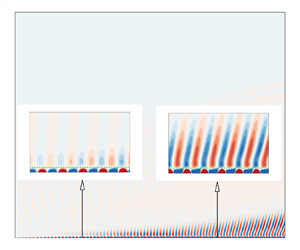
For the cold-wall condition, the supersonic mode is also found to be important. The phase distribution of (2.2)–(2.4) is investigated under the cold-wall condition for both the second and supersonic modes, as shown in figure 7(a,b). Here,  $Re=2000$ and $Re=2200$ correspond to the regions of the second mode and the supersonic mode, respectively. The second mode synchronises with the slow acoustic wave at $Re=2120$, which evolves into the supersonic mode downstream (Chuvakhov & Fedorov Reference Chuvakhov and Fedorov2016). As shown in figure 7(c), the supersonic mode radiates acoustic waves towards the far field, whose wave structure is essentially different from the second mode above the dashed line in figure 7(c). This region roughly corresponds to $Y>0.3$ in figure 7(b). For the supersonic mode in this region, what is less in phase with the rate of change of velocity or internal energy fluctuation is the wall-normal transport of the internal energy ( ${T_{T,{1}}}$). This decreased contribution of ${T_{T,{1}}}$ may be linked with the weaker instability of the supersonic mode compared with the second mode, which will be further checked by the Lagrangian approach.

Figure 7. Phase profiles of significant source terms in the regions of the second mode ( $Re=2000$) and the supersonic mode ( $Re=2200$) of (a) (2.2) and (b) (2.4). (c) Contour of pressure fluctuation of case 2. Dashed green line in (b,c) represents the location above which the structures of the supersonic and second modes clearly differ.
4. Connection with inviscid Lagrangian interpretation
Based on the DNS data, the time-averaged quantities of the source terms for case 1 and case 2 in (2.6) are depicted in figure 8. For case 1, as shown in figure 8(a), the dominant source term destabilising the second mode near the wall appears to be the DAP. The expression of DAP contains the components of fluctuations of dilatation and pressure gradient in (2.2)–(2.4). Therefore, the fact that DAP contributes to the growth of disturbance energy of the second mode near the wall is consistent with the significant role of fluctuations of dilatation and pressure gradient in RPA, as shown in figure 2(a–c). The RSS term keeps a nearly constant positive value inside the boundary layer, indicating a destabilisation effect on the second mode. The most pronounced contribution comes from the heat exchange term near the critical layer. This term is closely related to the internal energy fluctuation due to vertical transport, i.e.  ${T_{T,{1}}}$ (RTS) in (2.4). Replacing Kuehl's (Reference Kuehl2018) acoustic energy norm with Chu's energy norm, we obtain a more comprehensive understanding that the internal energy is mainly amplified along the critical layer while the acoustic energy is augmented in near-wall regions. The consistency with the RPA is also found.


For case 2, as shown in figure 8(b,c), the distribution of RSS for cold walls reports limited differences compared with the second mode in case 1. This finding is consistent with RPA in that wall cooling has no significant effect on RSS, as shown in figure 5(a). For the DAP, it is indicated that the region of DAP becomes relatively narrow under the cold-wall condition, which may be related to the appearance of the second GIP in the very near-wall region (see figure 4c). The contribution of the HE effect becomes not distinguished under the cold-wall condition for both second and supersonic modes near the critical layer. This may be relevant to the decreased base temperature gradient magnitude in the outer region, as shown in figure 4(b). Furthermore, the HE effect is augmented by wall cooling near the wall, which is consistent with the near-wall appearance of resonance between  $\bar \rho {{{\rm D} T'} / {{\rm D} t}}$ and ${T_{T,{1}}}$ in figure 5(b). The considerable reduction in the HE of the supersonic mode near the critical layer is also consistent with the explanation by RPA in figure 7(b). The transition from a strong second-mode instability to a weak supersonic-mode instability may be associated with the fact that the wall-normal HE (also ${T_{T,{1}}}$) is gradually out of phase with the internal energy fluctuation. The above observations indicate that RPA and Lagrangian energy analysis point to the same mechanisms for the inviscid high-frequency modes in hypersonic boundary layers.
5. Conclusion
The energy source terms of unstable modes over flat-plate boundary layers are investigated using RPA with various Mach numbers and wall temperature ratios. Through the phase analysis of source terms and changes of momentum and internal energy perturbations, the leading source terms of the T–S mode, the oblique first mode, the second mode and the supersonic mode are clarified, with considerations of porous coatings and obliqueness. It is found that contribution of the RSS is strengthened along with the distinctive oblique characteristic for the most unstable first mode, whereas that of the RTS is weakened for the second mode considering obliqueness. Wall cooling renders the fluctuations of RTS and dilatation out of phase with the rate of change of the internal energy fluctuation, thus stabilising the oblique first mode. However, a newly generated prominent region of wall-normal internal energy transfer, which is located underneath the second GIP, destabilises the second mode under wall cooling. As for the effect of porous coating, it stabilises the second mode in a manner comparable to wall heating while it destabilises the oblique first mode by enhancing mean-shear production in phase. Moreover, the wall-normal transport of internal energy at the critical layer becomes more out of phase for the significantly weaker supersonic mode, which accounts for the decreased contribution to energy growth. Connections and consistencies are highlighted with the inviscid thermoacoustic interpretation for the second and supersonic modes. The distinct sources in the critical layer and near-wall regions provide an in-depth understanding of the regional energy amplification processes of the inviscid modes in hypersonic boundary layers. Possible control strategies aimed at different modal properties are preliminarily discussed.
Acknowledgements
The authors would like to thank Professor X. Li for his generosity in providing the DNS codes, and Dr X. Tian for useful dicussions and suggestions.
Funding
This research is supported by the Research Grants Council, Hong Kong, under contract No. 15216621.
Declaration of interests
The authors report no conflict of interest.
Appendix A. Detailed formulae in stability equations
The expressions of  ${T_{u,{3}}}$, ${T_{v,{2}}}$ and ${T_{T,{3}}}$ are shown as follows, where Stokes’ hypothesis for the bulk viscosity is applied:
 \begin{align} {T_{u,3}} &= \frac{\bar \mu }{Re}\left[ { - \frac{4}{3}{\alpha ^2}\hat u + \frac{1}{3}({\rm{i}}\alpha \frac{{{\rm d}\hat u}}{{{\rm d}y}} - \alpha \beta \hat w) + \frac{{{{\rm d}^2}\hat u}}{{{\rm d}{y^2}}} - {\beta ^2}\hat u} \right] \nonumber\\ &\quad +\frac{1}{Re}\left[ {\frac{{{\rm d}\bar \mu }}{{{\rm d}y}} \left(\frac{{{\rm d}\hat u}}{{{\rm d}y}} + {\rm{i}}\alpha \hat v\right) + \frac{{{\rm d}\bar \mu }}{{{\rm d} \bar{T}}}\left(\frac{{{{\rm d}^2}\bar u}}{{{\rm d}{y^2}}}\hat T + \frac{{{\rm d}\bar u}}{{{\rm d}y}}\frac{{{\rm d}\hat T}}{{{\rm d}y}}\right) + \frac{1}{Re}\frac{{{{\rm d}^2}\bar \mu }}{{{\rm d}{\bar{T}^2}}}\frac{{{\rm d}\bar T}}{{{\rm d}y}} \frac{{{\rm d}\bar u}}{{{\rm d}y}}\hat T} \right], \end{align}
 \begin{align} {T_{v,{2}}} &= \frac{\bar \mu }{Re}\left[ { - {\alpha ^2}\hat v + \frac{1}{3} \left({\rm{i}}\alpha \frac{{{\rm d}\hat u}}{{{\rm d}y}} + {\rm{i}}\beta \frac{{{\rm d}\hat w}}{{{\rm d}y}}\right) + \frac{4}{3}\frac{{{{\rm d}^2}\hat v}}{{{\rm d}{y^2}}} - {\beta ^2}\hat v} \right] \nonumber\\ &\quad +\frac{1}{Re}\left[ {\frac{{{\rm d}\bar \mu }}{{{\rm d}\bar T}}\left({\rm{i}}\alpha \frac{{{\rm d}\bar u}}{{{\rm d}y}} + {\rm{i}}\beta \frac{{{\rm d}\bar w}}{{{\rm d}y}}\right)\hat T - \frac{2}{3}\frac{{{\rm d}\bar \mu }}{{{\rm d}y}} \left({\rm{i}}\alpha \hat u + {\rm{i}}\beta \hat w - 2\frac{{{\rm d}\hat v}}{{{\rm d}y}}\right)}\right], \end{align}
 \begin{align} T_{T,{3}} &= \frac{{\bar \mu \gamma }}{RePr}\left[ { - {\alpha ^2}\hat T + \frac{{{{\rm d}^2}\hat T}}{{{\rm d}{y^2}}} - {\beta ^2}\hat T + \frac{2}{\bar \mu } \frac{{{\rm d}\bar \mu }}{{{\rm d}y}}\frac{{{\rm d}\hat T}}{{{\rm d}y}}} \right] \nonumber\\ &\quad +\frac{\gamma }{RePr}\frac{{{{\rm d}^2}\bar \mu }}{{{\rm d}{y^2}}}\hat T + (\gamma - 1){M^2} \frac{1}{Re}\frac{{{\rm d}\bar \mu }}{{{\rm d}\bar T}}\left[ {{{\left(\frac{{{\rm d}\bar u}}{{{\rm d}y}}\right)}^2} + {{\left(\frac{{{\rm d}\bar w}}{{{\rm d}y}}\right)}^2}}\right]\hat T \nonumber\\ &\quad +2(\gamma - 1){M^2}\frac{\bar \mu }{Re}\left[{\frac{{{\rm d}\bar u}}{{{\rm d}y}}{{ \left(\frac{{{\rm d}\hat u}}{{{\rm d}y}} + {\rm{i}}\alpha \hat v\right)}^2} + \frac{{{\rm d}\bar w}}{{{\rm d}y}}\left({\rm{i}}\beta \hat v + \frac{{{\rm d}\hat w}}{{{\rm d}y}}\right)}\right]. \end{align}
Appendix B. Amplitude profiles
The amplitude distribution of the terms in (2.2)–(2.4) is also examined for further references. The variation of the amplitude profiles in the considered wide parameter space is calculated. In general, the amplitude distribution supports the existence of the significant source terms reported by the RPA in each parametric state. This finding is not surprising because consistency between the RPA and Lagrangian interpretation has been reached. The criterion of the Lagrangian interpretation is based on the amplitude magnitude.
In this section, the amplitude profiles of two representative states are shown, including the oblique first mode under an adiabatic wall condition in figure 9 and the second mode under a cold-wall condition in figure 10. Figure 9 illustrates that the amplitude of mean shear ( ${T_{u,{\rm {\ 1}}}}$) and RTS ( ${T_{T,{1}}}$) are pronounced across the boundary layer for the oblique first mode. The amplitude of viscous stress ( ${T_{u,{3}}}$) and viscous dissipation and thermal conduction ( ${T_{T,{3}}}$) becomes comparable to the rate of change in fluctuations below the critical layer. It is concluded that these distributions of amplitude magnitude support the significant source terms shown with RPA by figure 2 in the corresponding wall-normal region. For the second-mode behaviour in figure 10, the mean shear ( ${T_{u,{1}}}$) and streamwise gradient of pressure fluctuations ( ${T_{u,{2}}}$) report relatively large amplitudes below the critical layer compared with the amplitude of $\bar \rho {{{\rm D} u'} / {{\rm D} t}}$. For the sources of internal energy fluctuations, the amplitude of RTS ( ${T_{T,{1}}}$) near the critical layer and dilatation ( ${T_{T,{2}}}$) near the wall are comparable to that of $\bar \rho {{{\rm D} T'} / {{\rm D} t}}$. In addition, the newly generated source term ( ${T_{T,{1}}}$) near the wall due to wall cooling (see figure 5b) also shows a moderate amplitude. The amplitude of the viscous-associated terms become negligible for the second mode. All these amplitude observations show no inconsistency with the conclusions by RPA.


 Open access