


1. Introduction
When turbulence is present beneath a free surface, distinct surface features may be observed which are imprints of coherent motions underneath. Three characteristic types of features may be observed which, following Brocchini & Peregrine (Reference Brocchini and Peregrine2001), we refer to as ‘dimples’, ‘boils’ and ‘scars’. Dimples are roughly circular indentations caused by vertical vortices attached to the surface; boils are smooth areas elevated above the mean water level which signify an upwelling event at the edge of which trough-like scars appear, adjacent to curves of strong downdraught (see Muraro et al. Reference Muraro, Dolcetti, Nichols, Tait and Horoshenkov2021, for a fuller review). The imprints are particularly conspicuous in flows where the surface is relatively flat and unruffled by wind, and the turbulent motions are created in the bulk or bottom and rise to the surface, for instance in riverine flow; this is the situation we will consider.
It has been remarked in several investigations (e.g. Banerjee Reference Banerjee1994; Longuet-Higgins Reference Longuet-Higgins1996) that attached vortices often originate at the edges of upwelling boils where the surface divergence,  $\boldsymbol {\nabla }_\perp \boldsymbol{\cdot}{\boldsymbol u} = \partial _x u + \partial _y v=-\partial _z w$, is large and positive. Here ${\boldsymbol u}=(u,v,w)$ is fluid velocity in directions $(x,y,z)$ understood to be evaluated at the surface. Kumar, Gupta & Banerjee (Reference Kumar, Gupta and Banerjee1998) study the simultaneous population density of upwelling boils and vortices, and argue that the vortices are created by the upwellings. We here demonstrate that the number of surface-attached vortices at a given time is closely correlated with the mean-square surface divergence, with a time lag between them.
Small-scale turbulence near water surfaces strongly influences a number of processes which are vital to the Earth system. For instance, it affects the species selection and blooming of phytoplankton (Durham et al. Reference Durham, Climent, Barry, de Lillo, Boffetta, Cencini and Stocker2013; Lindemann, Visser & Mariani Reference Lindemann, Visser and Mariani2017), and the transport of pollutants such as microplastics (e.g. Jalón-Rojas, Wang & Fredj Reference Jalón-Rojas, Wang and Fredj2019).
Most significantly in our context, near-surface turbulence controls the transfer of gas between ocean and atmosphere by renewing the surface (Wanninkhof et al. Reference Wanninkhof, Asher, Ho, Sweeney and McGillis2009; D'Asaro Reference D'Asaro2014). Laboratory experiments (e.g. Herlina & Jirka Reference Herlina and Jirka2008; Turney & Banerjee Reference Turney and Banerjee2013), field studies (e.g. Veron, Melville & Lenain Reference Veron, Melville and Lenain2011) and numerical simulations (e.g. McCready, Vassiliadou & Hanratty Reference McCready, Vassiliadou and Hanratty1986; Kermani & Shen Reference Kermani and Shen2009; Khakpour, Shen & Yue Reference Khakpour, Shen and Yue2011) all show how the surface mass flux is closely linked to the root-mean-square (r.m.s.) surface divergence which we denote  $\beta (t)$ and define
 \begin{equation} \beta(t)^2 = \overline{(\boldsymbol{\nabla}_\perp\boldsymbol{\cdot}{\boldsymbol u})^2}= \overline{(\partial_z w)^2}, \end{equation}
where we use the convention that an overline denotes averaging over the  $(x,y)$ domain whereas $\langle \cdots \rangle$ signifies an average in time. Models of mass transfer have therefore often been based on $\langle \beta \rangle$ although a number of other alternatives have also been suggested as reviewed, e.g. by Banerjee (Reference Banerjee2007), including several based on some measure of the average time a fluid parcel stays at the surface before it is replaced (renewal time), $\langle \tau \rangle$.
A practical challenge is that neither  $\beta$ nor $\tau$ can be readily measured in the field. Although impressive field measurements of spatio-temporally resolved velocity fields centimetres beneath the surface have been made (e.g. Wang & Liao Reference Wang and Liao2016), they require highly advanced purpose-built set-ups, and are limited to measurements at a single site or along a trajectory. For measuring the topography of the turbulent free surface only, however, a range of advanced non-intrusive methods exist (Gomit, Chatellier & David Reference Gomit, Chatellier and David2022), in particular stereo imagery. Even simple shadowgraphs of a surface from a camera mounted on a drone have been used for remote sensing in a different setting (Streßer, Carrasco & Horstmann Reference Streßer, Carrasco and Horstmann2017). Non-contact measurement of riverine flow at larger length scales has been developed with infrared (Dugan et al. Reference Dugan, Anderson, Piotrowski and Zuckerman2013) and optical (Dolcetti et al. Reference Dolcetti, Hortobágyi, Perks, Tait and Dervilis2022) footage. If turbulence parameters which determine gas transfer rates, say, could be estimated even roughly by such means it would hold a high potential for surveying larger areas of the surface of lakes, rivers and oceans, quickly and at low cost.
The surface imprints of attached vortices have two particularly striking features: they are nearly circular, and they persist for a long time (Shen et al. Reference Shen, Zhang, Yue and Triantafyllou1999). We show how these physical traits combined allow simple and effective identification of vortex imprints on a turbulent free surface, by developing a simple, transparent and physics-based real-time computer vision technique able to identify and track surface-attached vortices purely from the dimples they create on the free surface. The method is tested on data from direct numerical simulation (DNS), showing accuracy and sensitivity both exceeding  $90\,\%$ without fine-tuning of parameters or further sophistication.
Our results suggest the possibility of estimating the rate of gas transfer across the free surface in natural flows remotely by inexpensive optical methods. Given the strong correlation between vortex number density and surface divergence, the former's prevalence could serve as proxy for the rate of gas transfer which is commonly parameterised in terms of  $\beta$ (Banerjee, Lakehal & Fulgosi Reference Banerjee, Lakehal and Fulgosi2004).
2. Methods and data
2.1. Numerical simulations
The data for analysis are obtained from a DNS of isotropic turbulence interacting with a deformable free surface. A statistically steady isotropic turbulence is generated by artificial forcing at the centre of the computational domain. The forcing is gradually reduced through a force-damping region as the free surface is approached, which allows the generated turbulence to propagate to a force-free near-surface region and excite free-surface motions. This set-up has been used by Guo & Shen (Reference Guo and Shen2010) to study the statistics of free-surface deformation and characterise the spatial–temporal behaviour of surface motions. The DNS utilises a time-dependent surface-fitted grid to resolve the deformable free surface. The detailed numerical scheme and validations can be found in Xuan & Shen (Reference Xuan and Shen2019). It has been verified that the simulation satisfies the resolution requirement of DNS (Xuan & Shen Reference Xuan and Shen2022).
The simulations are set up in dimensionless quantities. The dimensionless domain size is set to  $L \times L \times \bar {H} = 2 {\rm \pi}\times 2 {\rm \pi}\times 5 {\rm \pi}$, where $L$ is the horizontal domain length and $\bar {H}$ is the mean water depth; this implicitly sets the characteristic length scale for non-dimensionalisation to $1/(2{\rm \pi})$ of the physical horizontal domain length. The characteristic time scale is set by the strength of the forcing for generating the isotropic turbulence (Xuan & Shen Reference Xuan and Shen2022, table 1), which determines a time scale over which energy is injected into isotropic turbulence. The dimensionless kinematic viscosity $\nu$ is set to $4\times 10^{-4}$. The r.m.s. velocity fluctuation of the simulated turbulence, evaluated at a distance of ${\rm \pi} /4$ from the free surface, is $u_{rms}=0.125$; the Reynolds number based on the Taylor microscale is ${Re}_{\lambda } = u_{rms} \lambda / \nu \approx 56$ where the Taylor microscale is $\lambda = u_{rms} \sqrt {15\nu /\varepsilon }=0.180$ with $\varepsilon =2\nu \langle \mathrm {Tr}(\boldsymbol{\mathsf{S}}^2)\rangle$ with $S_{ij}=(\partial _iu_j+\partial _ju_i)/2$ and $\mathrm {Tr}$ denoting the trace; the integral length scale is $L_\infty = \lambda Re_\lambda /15= 0.67$; and we define an integral time scale as $T_\infty =L_\infty /u_{rms} = 5.41$. The Froude number is $Fr=u_{rms}/\sqrt {g L_\infty }=0.048$, where g is the gravitational acceleration. Surface tension is set to zero in the present study. The data set exported for analysis has a time step $\Delta \tau =0.060$ between consecutive frames.
2.2. Wavelet analysis
Wavelets, a building block of computer vision techniques, are particularly suitable for detection of localised intermittent structures, and have been used for bulk turbulence for a long time (e.g. Farge Reference Farge1992; Schram, Rambaud & Riethmuller Reference Schram, Rambaud and Riethmuller2004). A few studies used wavelets for surface wave analysis (Dolcetti & García Nava Reference Dolcetti and García Nava2019), and very recently a wavelet-based surface feature tracking technique was demonstrated in the laboratory by Gakhar, Koseff & Ouellette (Reference Gakhar, Koseff and Ouellette2022). Another approach to inferring bulk flow from surface information is machine learning, recently demonstrated by Xuan & Shen (Reference Xuan and Shen2023); machine learning is a powerful predictive technique whereas the technique presented here is conceptually simple and physically transparent at every step, so the two approaches can be considered complementary.
Let  ${\boldsymbol x}=(x,y)$ be a position in the horizontal surface plane and $\eta ({\boldsymbol x},t)$ the free-surface elevation at time $t$. The two-dimensional continuous wavelet transformation, $W$, is found by taking a convolution between $\eta ({\boldsymbol x},t)$ and a mother wavelet, $\psi ({\boldsymbol x})$ (Antoine et al. Reference Antoine, Murenzi, Vandergheynst and Ali2008), reading in the case of a real-valued wavelet,
 \begin{equation} W_{s, \theta}({\boldsymbol x};t) = \int_{R^2} \eta({\boldsymbol \xi},t) \psi\left(\frac{{\boldsymbol x}-{\boldsymbol \xi}}{s},\theta\right) \,\mathrm{d}{\boldsymbol \xi}, \end{equation}
where  $s$ is a scaling parameter for the wavelet, ${\boldsymbol \xi }$ is a position vector and $\theta$ a rotation angle. A large range of different mother wavelets are in standard use (see Antoine et al. Reference Antoine, Murenzi, Vandergheynst and Ali2008), yet the simple axisymmetric Mexican hat, defined as
 \begin{equation} \psi({\boldsymbol x},\theta) = \psi(x) = (x^2-2)\mathrm{e}^{-x^2/2} \end{equation}
with  $x=|{\boldsymbol x}|$, performs well for our purposes and is preferable for its calculational efficiency.
The choice of an axisymmetric wavelet is intuitive because the structures we wish to detect are approximately circular indentations; the transformation involves a convolution of signal and wavelet, so similarity of shape between signal and wavelet produces the strong spectral peaks from which the size and position of surface imprints can be determined. We use MATLAB Wavelet Toolbox algorithms to compute the wavelet transform.
3. Vortex detection from free-surface features
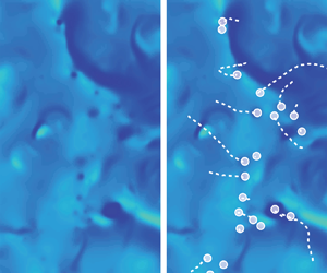
The vortex detection algorithm proceeds as illustrated in the panels of figure 1 for a typical time step. Colourbars are omitted in panels (a–c,f–h) since the figure is qualitative. Details about individual steps and how threshold values are determined are given in § 3.1.

Figure 1. Qualitative illustrations of steps in vortex identification of vortices, slightly simplified (time step no.  $1465$ from DNS data for illustration). (a) Input, surface elevation $\eta$; (b) wavelet transform $W(x,y)$ of $\eta$; (c) regions where $W>W_{thr}$; (d) calculated eccentricity of each structure (five examples given), high eccentricity structures discarded (marked with cross); (e) time-tracking showing trajectories of area centres from birth to present time, short-lived structures discarded (crosses); (f) output, surface elevation and tracked vortices; (g–i) show steps in performance evaluation; (g) the value of $\lambda _2$ at the surface; (h) areas with $\lambda _2<\lambda _{2,{thr}}$ (potential ‘true’ vortices) as defined and detailed in § 3.2.1; (i) detections (circles/trajectories) and actual real vortex cores (blue). Note in (c,h,i) the structure marked with an arrow, discarded due to high eccentricity (d) is in fact a cluster of vortex cores; a few time steps later it splits in two whereupon both halves are detected. See also supplementary movie 1 available at https://doi.org/10.1017/jfm.2023.370).
In summary the procedure is as follows. For each time step  $n$, the surface elevation $\eta ({\boldsymbol x},t)$ (figure 1a) is transformed to a wavelet spectrum $W_{s}({\boldsymbol x};t)$ using the 2-D-Mexican hat wavelet (2.2) with a set scale $s$ (figure 1b); a threshold $W_{thr}$ is applied to isolate surface features as connected regions with strong positive values, $W_{s}>W_{thr}$, which are then labelled (figure 1c). Tracking in time is achieved by identifying connected regions which overlap between frames $n-1$ and $n$ as one and the same, adding to the corresponding feature's lifetime measured from first detection. The eccentricity (deviation from circularity) of each region is found (figure 1d). The following features are now declared dead: those whose connected regions in time step $n-1$ without an overlapping region in step $n$, and whose eccentricity averaged over the last few time steps is above a maximum value $\epsilon _{max}$. Features whose lifetime $\tau$ is less than a minimum $\tau _{min}$ are discarded as ‘not a vortex’ (figure 1e). Structures which are retained beyond the minimum lifetime we refer to as ‘detections’.
To measure performance, ‘true’ vortices (as defined below) were identified from the surface velocity field (figure 1g,h) based on a criterion given below, allowing false positives and negatives to be identified and accuracy and sensitivity to be calculated.
The algorithm described has the property of making a single pass through the data using only the current image frame and a few preceding it, and can be employed continuously (real time) as data are acquired. There are several straightforward ways by which the method can be further improved to remove typical types of false positives and negatives (some observations are mentioned below). A fully optimised detection algorithm is not our goal here, however; a machine learning approach such as Xuan & Shen (Reference Xuan and Shen2023) could be a better approach if so. We wish instead to highlight the transparent physics and emphasise how a simple selection based only on two physical properties, lifetime and eccentricity, can be highly effective.
3.1. Algorithmic details and parameter values determination
The algorithm involves determining appropriate values of four parameters:  $s,W_{thr},\tau _{min}$ and $\epsilon _{max}$. We discuss them in the following and propose methods based on experience as well as physics, by which these can all be chosen using surface elevation data.
3.1.1. Wavelet scale
Unlike eddy detection in bulk turbulence (e.g. Schram et al. Reference Schram, Rambaud and Riethmuller2004), determining an appropriate wavelet scale is straightforward in our case: the vortex imprints are relatively uniform in size, easy to identify by eye, and detection is not highly sensitive to choice of scale. The smallest scale of the Mexican hat vortex is related to the Nyquist frequency, i.e. the smallest wavelet that the grid can resolve (contained within  $3\times 3$ grid points); $s=1$ in our terminology. The upper scale limit is not relevant for our purposes. The appropriate scale will depend on the spatial resolution of the data. In our case the vortex imprints were small enough that the smallest wavelet scale was chosen. The scales $s=2$ and $4$ were also tested. The results with the former are equally good for our purposes, as shown in figure 2(c): the difference in cumulative lifetime is insignificant, and the difference in the cumulative number of vortex detections is mainly that with the two larger scales, one and the same feature is occasionally ‘lost’ and ‘found again’ and thus counted as two or more separate detections. The cumulative lifetime deviates somewhat with s = 4, but not dramatically so.

Figure 2. (a) Scatter plot of all detected regions ( $W_s>W_{thr})$ by lifetime and average eccentricity, colour coded according to whether it corresponds to a true vortex (no lifetime threshold). The very shortest-lived regions are not shown. The ordinate axis is scaled as $-\log(1-\epsilon)$. (b) Coverage as a function of wavelet transform cutoff $W_{thr}$ (linear and logarithmic scale, respectively). (c) Cumulative vortex number and lifetime as a function of time step for three different vortex scales. (d) Number (black) and lifetime (orange) of all retained regions with $\tau \geq \tau _{min}$ with eccentricity filtering (i.e. detections) and without. (e) Accuracy and sensitivity as a function of $\tau _{min}$. Dotted horizontal and vertical lines indicate the threshold values used: vertical lines show $\tau _{min}=0.166T_\infty$ in (a,d,e) and $W_{thr}=0.00015$ in (b); horizontal dashed line in (a) is $\epsilon _{max}=0.85$.
As an example of how the wavelet transform highlights features whose physical size is similar to their own, the wavelet spectrum of the surface elevation in figure 1(a) is shown in figure 1(b). For a low value of  $s$, sharp gradients give a strong signal $|W_s|$ whereas the structures that are much larger than the wavelet are overlooked. Only the edges of the largest coherent structures show up in the spectrum as elongated shapes with high eccentricity.
3.1.2. Wavelet spectrum threshold
Imprints of vortices have negative values of surface elevation, corresponding to positive  $W_{s}$ in our formulation. We find that an appropriate value of $W_{thr}$ can be determined by regarding the coverage, i.e. the relative portion of the surface which satisfies $W_{s}({\boldsymbol x};s)>W_{thr}$. Figure 2(b) shows coverage averaged over all frames as a function of $W_{thr}$. In a narrow range of $W_{thr}$ values, coverage drops suddenly from close to $1$ to $\ll 1$. After this drop, the most energetic features in the transform remain, corresponding to the features of interest. To appropriately capture them, the threshold should be set low enough that the coverage is several times that of the detected vortices that remain after subsequent filtering. The value we used was $W_{thr}=1.5\times 10^{-4}$ giving a coverage of approximately $2.5\,\%$ while the coverage from those retained after filtering (detections) is $0.36\,\%$. The universality of these values is difficult to assess from a single data set, yet we propose that a criterion based on coverage to determine an appropriate $W_{thr}$ is a broadly applicable approach.
3.1.3. Maximum eccentricity
Comparing figure 1(c,h) we see that most of the connected regions found from wavelet thresholding which are not imprints of vortices are strongly elongated in shape. A suitable measure of the departure from circularity is eccentricity.
Consider a connected region consisting of points in an area  $A_c$. The eccentricity of $A_c$ is
 \begin{equation} \epsilon = \sqrt{1-(\varLambda_2/\varLambda_1)}, \end{equation}
where  $\varLambda _1$ and $\varLambda _2$ are, respectively, the largest and smallest eigenvalue of the intensity covariance matrix (indices $i,j\in \{x,y\}$)
 \begin{equation} \sigma_{ij} = \int_{A_c} \tilde x_i \tilde x_j W_{s}({\boldsymbol x})\,\mathrm{d} {\boldsymbol x}, \end{equation}
where  $A_c$ is the area of the detected structure in question, and $\widetilde {{\boldsymbol x}}={\boldsymbol x}- {\boldsymbol x}_c$ with the centroid, ${\boldsymbol x}_c = A_c^{-1}\int _{A_c}{\boldsymbol x}\,\mathrm {d} {\boldsymbol x}$. A perfectly circular area has $\epsilon =0$ whereas $\epsilon \to 1$ for increasing deviation from circularity. The eccentricity of five example regions are given in figure 1(d). Since also true vortices can undergo short periods of higher eccentricity, we base the filtering on $\epsilon$ averaged over the previous few time steps – we use the preceding $\tau _{min}/3$, but sensitivity and accuracy are not sensitive to the exact choice of interval. Features whose $\epsilon$ exceeds $\epsilon _{max}$ are declared dead (discarded as not a vortex if the minimum lifetime is not reached).
The value  $\epsilon _{max}=0.85$ is found to be appropriate as figure 2(a) illustrates: the vast majority of true vortices have average eccentricity less than $0.85$ and vice versa for detected regions which are not vortices. While pragmatically chosen, we propose that this value will be a reasonable choice quite generally. (Note, figure 2(a) uses $\epsilon$ averaged over the whole lifetime.)
3.1.4. Minimum lifetime
When the minimum lifetime threshold  $\tau _{min}$ is increased from zero, the number of detected regions drops rapidly as figures 2(a) illustrates and 2(d) quantifies. A value is chosen where the dropoff becomes less steep. Beyond the point where the graph has the strongest curvature, sensitivity and accuracy are fairly insensitive to the exact value chosen. See further discussion in § 3.2.1. We used $\tau _{min}=0.166T_\infty$
3.2. Performance and correlations with surface divergence
To evaluate sensitivity and accuracy (S&A) it is necessary to identify features erroneously identified as vortices, and vortices which are not detected. These are called false positives ( $FP$) and false negatives ( $FN$), respectively. True positives ( $TP$) are either ‘true vortices which are detected’ (superscript $(t)$) or ‘detections which are true vortices’ (superscript $(d)$). The combined lifetime of the elements (indexed $i=1,\ldots,N$) in each category, $\mathcal {T}=\sum _{i=1}^N \tau _i$, is a better measure than their total number $N$, since ratios between them measure the ability to correctly count the number of vortices present at a given point in time. When a vortex is momentarily ‘lost’ from sight and ‘found’ again it is counted as two detections as discussed in connection with figure 2(c), but the total lifetime – and hence S&A – is little affected. Sensitivity measures the ratio of true vortices which are detected, $\mathcal {T}_{TP}^{(t)}/(\mathcal {T}_{TP}^{(t)}+\mathcal {T}_{FN})$; accuracy measures the ratio of detections which are true vortices, $\mathcal {T}_{TP}^{(d)}/(\mathcal {T}_{TP}^{(d)}+\mathcal {T}_{FP})$. (The concept of true negatives is not meaningful here.) In general $\mathcal {T}_{TP}^{(t)}$ and $\mathcal {T}_{TP}^{(d)}$ are not identical; with our parameters they are within a few per cent of each other.
3.2.1. True vortices, accuracy and sensitivity
True vortices are identified using the velocity field on the fluid surface. The criterion of Jeong & Hussain (Reference Jeong and Hussain1995) is that a point belongs to a vortex core if the median eigenvalue  $\lambda _2$ of the matrix $\boldsymbol{\mathsf{S}}^2-\boldsymbol{\mathsf{W}}^2$ is negative; here $W_{ij}=(\partial _iu_j-\partial _j u_i)/2$ is the vorticity tensor. The centres of surface-attached vortices have large, negative $\lambda _2$.
We define true vortices as connected regions wherein  $\lambda _2< \lambda _{2,{thr}}$ with $\lambda _{2,{thr}}=-2$ and persists for at least a time $\tau _{true,min}$ with an area of at least two grid points. We choose $\tau _{true,min}=\tau _{min}=0.166 T_\infty$. These limits are pragmatic and mean that extremely short-lived or tiny structures are outside what we wish to detect. The area of a vortex detection must overlap with that of a true vortex during ${\geq}40\,\%$ of its lifetime to be considered correct, and vice versa for a vortex to be considered detected. Figure 1(g–i) shows $\lambda _2(x,y)$ at the free surface, illustrating how detected regions correspond to regions with large negative $\lambda _2$.
Figure 2(e) shows that the simple detection procedure gives S&A well over  $90\,\%$ for a wide range of minimum lifetimes, $0.7\lesssim \tau /T_\infty \lesssim 2.5$. The eccentricity filter excludes the vast majority of negatives, whereupon S&A are relatively insensitive to the choice of $\tau _{min}$; even though the number of detections falls by approximately $50\,\%$ in this range, those discarded are so short-lived that the cumulative lifetime is only decreased by $14\,\%$.
We mention in passing three further criteria which can easily be used to remove common types of false positives. The vortex candidate's centroid  ${\boldsymbol x}_c$ should lie within its area $A_c$ and/or $A_c$ should not be much smaller than that of the smallest circle which circumscribes it; this removes edges of upwelling regions which although very thin and elongated, happen to curve into a ring-like shape of low eccentricity. Finally, if a detected area $A_c$ is a true positive, its centroid ${\boldsymbol x}_c(t)$ moves along a smooth path whereas that of false positives typically follows a jagged path with sharp corners.
3.3. Correlations with surface divergence
It was remarked by Banerjee (Reference Banerjee1994) that a relation must exist between the number of attached vortices and upwelling events, which are associated with strong surface divergence. Shen et al. (Reference Shen, Zhang, Yue and Triantafyllou1999) provide a detailed description of the primary causal mechanism that links the two. By tracing vortex lines they show how hairpin-like vortices beneath the surface are swept upwards by the rising fluid during strong upwelling. Owing to the dissipation and stretching of the horizontal vorticity near the free surface, the hairpin vortex breaks up and the legs attach to the surface, a vortex of ‘Type A’ as characterised and described in the review of Sarpkaya (Reference Sarpkaya1996). The attached vortices are pushed outward to the periphery of the upwelling boil by its outward surface flow. A significant rise in averaged positive surface divergence signifies a strong upwelling event, hence can be expected to be followed by an increase in the number of surface-attached vortices.
In figure 3 we show quantitatively that the mean-square of the surface divergence,  $\beta (t)^2$, is closely correlated with the number of vortex detections in the domain, $N(t)$. Peaks in $N(t)$ lag a little behind the corresponding maxima of $\beta (t)^2$, in concordance with the observation that vortices gradually appear around a strong upwelling event. The normalised cross-correlation (NCC) between the two time series after their respective average values are subtracted, shown in figure 3(b), peaks at $0.90$ for a lag of approximately $0.8\,T_\infty$. Using true vortices (as defined) rather than detections gives essentially identical results. Our data strongly indicates that the cross-correlation between $N(t)$ and $\beta (t)^q$ is greatest for $q=2$. (The maximum NCC was found for $q=1.944$ and is only $0.01\,\%$ higher than for $q=2$; this difference is clearly less than our uncertainty.)

Figure 3. (a) Plot of the mean-square surface divergence (surf. div.) against the number of detected vortices. (b) The NCC between the two (average values subtracted) as a function of lag, peaking at  $0.90$ with lag $0.80\, T_\infty$.
Held together, our two main results point to an exciting prospect: surface-attached vortices can be easily identified from their surface imprints and their number is intimately correlated with surface divergence – hence also with gas transfer – suggesting that gas transfer rates might be estimated remotely by using dimples on the free surface as proxy.
3.3.1. Dependence on turbulent flow conditions
We have considered a single DNS with  ${Re}_{\lambda } \approx 68$, $Fr=0.048$, as defined in § 2.1. Another dimensionless group that characterises the behaviours of free surfaces is the Weber number $We=\rho u_{rms}^2 L_\infty /\gamma$, with $\rho$ the fluid density and $\gamma$ the surface tension; in the present study, the surface tension is not considered, i.e. $We\to \infty$. We will briefly discuss the significance of these key non-dimensional groups to our method and physical observation.
The ability of subsurface turbulence to leave imprints on the free surface is governed by the Froude and Weber numbers, which express the ability of the restoring forces of gravity and surface tension, respectively, to counter the surface motion from turbulent flow inertia. Following the analysis by Brocchini & Peregrine (Reference Brocchini and Peregrine2001), the dimples, boils and scars are prevalent when gravity is dominating and surface tension is weak (denoted ‘Region 3’ in their figure 4), characterised by  $Fr\ll 1$ and $We\gg 1$; it is, they state, by far the commonest condition in natural flows.
Increasing surface tension (i.e. lowering  $We$) tends to smooth out the smaller features of the free-surface imprint (Guo & Shen Reference Guo and Shen2010), roughly those of characteristic sizes smaller than $O(Fr/\sqrt {We})$. How a finite We would affect our conclusions is a question we relegate to future study. When $Fr$ and $We$ are both large, the surface will eventually disintegrate through droplet formation and/or air entrainment; our procedure clearly is not applicable under such conditions. The Reynolds number governs the nature of the turbulent structures beneath the surface; higher $Re$ will mean a greater range of eddy sizes and stronger intermittency. It should also be pointed out that the strengthening of the vertical vorticity is mainly attributed to vortex stretching and turning (Walker, Leighton & Garza-Rios Reference Walker, Leighton and Garza-Rios1996; Zhang, Shen & Yue Reference Zhang, Shen and Yue1999). The viscous dissipation of the vorticity is reduced considerably once vortices attach to the surface (Shen et al. Reference Shen, Zhang, Yue and Triantafyllou1999). This suggests the relatively weak role of the viscous effect in the evolution of surface-attached vertical vortices. While the ability of subsurface turbulence to leave imprints on the surface is not governed by $Re$ directly, in practical situations for a given fluid $Re, We$ and $Fr$ are all determined by the turbulent motion and difficult to control independently (turbulence generation with an active grid allows some independent control of turbulence intensity and integral scale; see Smeltzer et al. Reference Smeltzer, Rømcke, Hearst and Ellingsen2023).
We do not consider the effect of wind, acting on the surface, via shear stress and form drag. In this case, the wind causes its own imprints on the surface, such as wrinkles, streaks and ripples, which can obscure those created by the subsurface turbulence, and new physical phenomena are introduced (see e.g. Rashidi & Banerjee Reference Rashidi and Banerjee1990 who performed experiments both with and without wind shear, and the recent numerical investigation of Li & Shen Reference Li and Shen2022). The study of such a situation is beyond our scope.
4. Conclusions
We consider the twin questions of how surface-attached vortices in free-surface turbulence can be identified from their surface imprints only, and how in turn they correlate with surface divergence, a key quantity in models of gas transfer across the surface. Using DNS data as a testbed, we develop a simple computer vision method able to correctly identify attached vortices with sensitivity and accuracy both well in excess of  $90\,\%$ (according to definitions detailed herein). The method is physically transparent and, after initial detection of all imprints of a certain strength and range of length scales, distinguishes vortex imprints from other surface features only by using two well-known physical properties of surface-attached vortices: their imprints are roughly circular depressions and they persist for a long time. We discuss how threshold values can be determined from the data itself.
The quoted performance metrics are obtained purely by filtering out imprints whose eccentricity is higher than a threshold, and lifetime is shorter than a minimum, with no further sophistication or fine-tuning of parameters. A physical insight is how distinct vortex imprints are on the turbulent free surface. In plain language, if it looks like the imprint of a vortex, it almost certainly is one: a persistent, circular surface depression is highly likely to be the surface end of a vortex core.
A close correlation is found between the development in time of the number of vortices present and the mean-square surface divergence. The NCC between the two time series peaks at  $0.90$ with changes in the number of vortices occurring a little less than one integral time unit (the turbulence integral length scale divided by the r.m.s. turbulent velocity) after the corresponding change in surface divergence quantifying the oft-observed tendency of vortices to originate around the edge of intermittent upwelling events.
Held together, the ease with which vortices can be automatically identified from their surface imprint, and their close correlation with surface divergence, suggests an exciting possibility of estimating the rate of gas transfer across a turbulent surface remotely.
Supplementary movie
Supplementary movie is available at https://doi.org/10.1017/jfm.2023.370.
Supporting simulation data and codes available from Babiker et al. (Reference Babiker, Bjerkebék, Ellingsen, Shen and Xuan2023).
Acknowledgements
O.M. and S.Å.E. have benefited greatly from discussions and suggestions from the other members of our research group, especially Drs O. Rømcke and B.K. Smeltzer.
Funding
S.Å.E. is funded by the European Union (ERC, WaTurSheD, grant 101045299) and the Research Council of Norway, grant 325114. Views and opinions expressed are, however, those of the authors only and do not necessarily reflect those of the European Union or the European Research Council. Neither the European Union nor the granting authority can be held responsible for them. The research of A.X. and L.S. is supported by the Office of Naval Research and National Science Foundation.
Declaration of interests
The authors report no conflict of interest.


 Open access