1. Introduction
1.1. Motivation
In order for magnetically confined plasmas to reach fusion power producing conditions, some form of auxiliary heating will be required. Furthermore, even under fusion burn conditions, external systems may likely be required to control the plasma and current profiles. While many different auxiliary heating and control schemes are available for present day devices, not all schemes extrapolate easily to the high density, high magnetic field devices that are envisioned for a fusion reactor. In some cases, advances in engineering such as increased energy for neutral beams or high-frequency sources for electron cyclotron heating, are leading to practical solutions. On the other hand, the cost-effective technology for sources in the ion cyclotron range of frequencies (ICRF) in reactor relevant devices is already available. Furthermore, the flexibility and efficiency of ICRF heating schemes and their availability for other applications including current drive, sawtooth stabilization and even wall conditioning among others, is notable. One of the challenges for employing ICRF power in present day and future devices lies in the interaction of the waves with the plasma boundary, vessel walls and other material surfaces. The reason is not difficult to understand intuitively. The wavelength of ICRF waves, typically in the frequency range of 30–100 MHz, is long compared with the wavelength of lower-hybrid or electron cyclotron frequency waves. ICRF wavelengths can approach or even exceed wall-to-edge plasma dimensions in the boundary region. As a result, ICRF waves can intuitively be expected to spread throughout the device and interact with the device walls, especially if the central plasma absorption is weak. Even without such ‘far-field’ effects, ICRF waves can interact strongly with launching structures in the near field since ICRF launchers must be placed in sufficiently high-density plasma for good coupling whereas higher-frequency waves can propagate through a low-density scrape-off layer plasma or even through a vacuum region.
1.2. Historical background and context
A radio frequency (RF) sheath is a narrow region surrounding a material surface, where a non-neutral plasma and large amplitude RF wave fields coexist. The RF sheath width, typically of the order of 10 or more Debye lengths in extent, is small compared with the plasma radius. A sheath may be considered an RF sheath when the RF waves are of sufficient amplitude to control the properties of the sheath itself; namely, the RF waves give rise to sheath voltages which exceed the thermal sheath voltage. RF sheaths have been implicated in ICRF boundary plasma–material surface interactions for some time. Various aspects of ICRF boundary plasma interactions from an experimental viewpoint are reviewed in Noterdaeme & Van Oost (Reference Noterdaeme and Van Oost1993) and early attempts at theory and modelling are briefly reviewed in Myra et al. (Reference Myra, D'Ippolito, Russell, Berry, Jaeger and Carter2006). The main experimental signatures of these interactions were: (i) the release of impurities by RF enhanced sputtering from surfaces, and (ii) parasitic power loss, i.e. wave power was not efficiently reaching the core, but rather appeared to be lost in the edge. We will see that RF sheaths provide a natural explanation for both phenomena.
Long before RF sheaths became of interest in fusion plasmas, they were studied in small-scale plasma discharge devices. The important process of voltage rectification by an RF sheath was recognized in Butler (Reference Butler and Kino1963). Modelling of rectification is of great interest for fusion plasmas and will be discussed in detail in several subsequent sections of this tutorial. It is the process by which the sheath generates a direct current (DC) voltage from an oscillating RF voltage. The resulting DC voltage drop between the plasma and the wall accelerates positively charged ions into the wall at high energy. This in turn results in greatly enhanced sputtering of wall materials (impurities) into the plasma.Footnote 1
As the ICRF fusion community began to recognize the importance of RF sheath rectification, numerical models were developed using one-dimensional fluid and Vlasov models (Chodura & Neuhauser Reference Chodura and Neuhauser1989; Perkins Reference Perkins1989; Brambilla et al. Reference Brambilla, Chodura, Hoffman, Neuhauser, Noterdaeme, Ryter, Schubert and Wesner1990; Myra, D'Ippolito & Gerver Reference Myra, D'Ippolito and Gerver1990). Early zero-point models of impurity sputtering based on these considerations were also developed (D'Ippolito et al. Reference D'Ippolito, Myra, Bures and Jacquinot1991) and applied to describe ICRF impurity release in experiments on JET (Bures et al. Reference Bures, Jacquinot, Lawson, Stamp, Summers, D'Ippolito and Myra1991). In some of those experiments, it was argued that the conditions for a self-sputtering avalanche may have occurred: the acceleration of an impurity ion in the sheath gave it an energy at which more than one impurity ion was sputtered from the surface and returned to it to re-sputter resulting in a positive feedback loop.
Strong ICRF interactions with the antenna and other surfaces were frequently observed in almost all experiments employing ICRF heating. Infrared camera images provided detailed maps of the ‘hot spots’ on the antenna and surrounding structures where high temperatures were measured resulting in surface damage such as the flaking of coatings. Colas et al. (Reference Colas, Costanzo, Desgranges, Brémond, Bucalossi, Agarici, Basiuk, Beaumont, Bécoulet and Nguyen2003) A particularly illuminating example from Tore Supra is shown in figure 1.
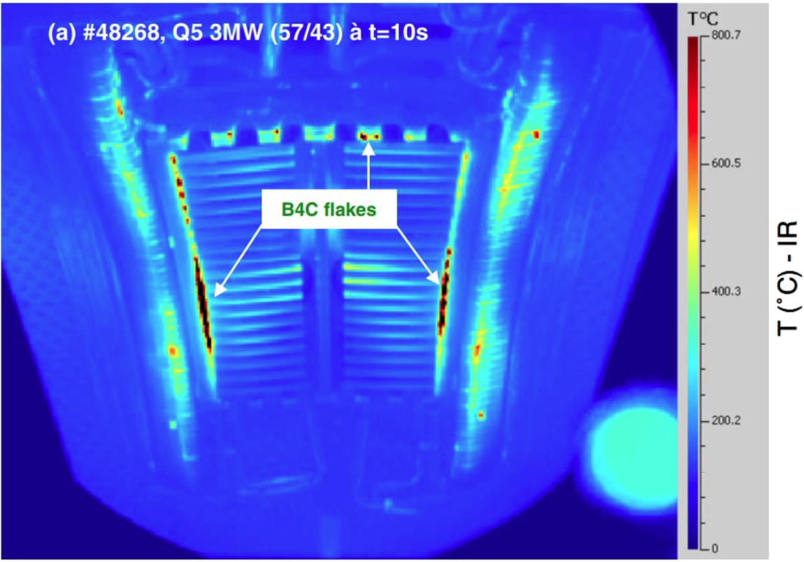
Figure 1. Infrared image of a Tore Supra ICRF antenna powered at 3 MW, showing high temperature ‘hot spots’ resulting in flaking of the B4C coating. Reprinted by permission from figure 6(a) of Corre et al. (Reference Corre, Firdaouss, Colas, Argouarch, Guilhem, Gunn, Hamlyn-Harris, Jacquot, Kubic, Litaudon, Missirlian, Richou, Ritz, Serret and Vulliez2012).
Excessive power reaching various surfaces surrounding an antenna can increase the heat flux on those surfaces to the point where material damage occurs. The most affected surfaces may be the ones exposed to the highest combination of RF power and plasma density. It was found in the experiments on Tore Supra and in other experiments on JET that a related consequence of RF rectification is the formation of RF-induced convective cells (D'Ippolito et al. Reference D'Ippolito, Myra, Jacquinot and Bures1993; Bécoulet et al. Reference Bécoulet, Colas, Pécoul, Gunn, Ghendrih, Bécoulet and Heuraux2002; Colas et al. Reference Colas, Ekedahl, Goniche, Gunn, Nold, Corre, Bobkov, Dux, Braun, Noterdaeme, Mayoral, Kirov, Mailloux, Heuraux, Faudot and Ongena2007). RF-driven convection from E × B drift occurs when DC (RF rectified) potentials vary from one magnetic field line to the next. (Here E is the RF electric field and B is the background magnetic field.) RF-driven convection will be discussed in more detail in § 6. It can increase or decrease the plasma density and hence the power deposition at a surface depending on its flow direction.
There are many more examples of important fusion-relevant experiments and modelling, some of which will be referenced later in this article. The few mentioned here should be sufficient to motivate the topic of RF sheaths.
Before moving on, it is well to note that RF sheaths are of practical interest in other contemporary applications besides ICRF heating or current drive in fusion plasmas. A companion body of research on RF sheaths may be found in the plasma processing literature. Some examples are the capacitive sheath studies in Lieberman & Godyak (Reference Lieberman and Godyak1998) and (Godyak & Sternberg Reference Godyak and Sternberg1990). Additional material may also be found in Gekelman et al. (Reference Gekelman, Barnes, Vincena and Pribyl2009) and Jaeger et al. (Reference Jaeger, Berry, Tolliver and Batchelor1995) and in the review of capacitively coupled plasmas in Donkó et al. (Reference Donkó, Schulze, Czarnetzki, Derzsi, Hartmann, Korolov and Schungel2012). References relevant to model specific issues will be given later.
While RF sheath physics in plasma processing devices shares some important fundamentals with RF sheaths in fusion plasmas, there are also some important distinctions. The first and foremost is probably the presence of a strong magnetic field in the fusion case and the common occurrence of magnetic field lines that are incident obliquely on a surface. Magnetic fields are used in plasma processing devices as well, but much of the literature that deals with RF sheaths is for semi-conductor etching applications where the magnetic field is either absent or is normal to the surface. As we will see, in that case it has little effect on the sheath dynamics. Additionally, other relevant parameters such as plasma density, temperature and RF frequency may be in different regimes in the two cases. RF discharge plasma devices are usually smaller in size than plasma fusion devices. Consequently, the former are almost always concerned with near-field RF interactions. In contrast, surface interactions with propagating waves are also of interest in tokamaks and other large-scale devices. Finally, neutral–plasma interactions and plasma chemistry are frequently important if not the primary goal in plasma processing applications. This physics can be important in fusion plasmas as well when impurity or fuelling modelling is sought, but such considerations are not of prime relevance to the structure of the RF sheath itself.Footnote 2 Perhaps the most significant difference between the two fields is in the modelling outputs that are of interest. In both applications, RF sheath rectification and power dissipation may be of interest. However, in fusion devices, the reaction of the RF wave fields that created the sheath on the sheath itself is of importance since it may determine the fraction of RF power that ultimately makes it into the core for its intended purpose and the remaining power that ends up damaging material surfaces.
Another field of study which has some overlap with the present tutorial is that of probes; see Demidov et al. (Reference Demidov, Koepke, Kurlyandskaya and Malkov2020), Hutchinson (Reference Hutchinson2005) and Shun'ko (Reference Shun'ko2008). Probes are often employed to measure plasma properties in magnetic fusion devices and an understanding of probe sheaths is critical to interpretation of the data they produce. An applied probe voltage can be swept with respect to the plasma potential to measure the current–voltage characteristic from which it is possible to extract the plasma density and temperature. If the sweeping frequency is sufficiently low compared with a characteristic sheath frequency (usually the ion plasma frequency), the sheaths are of the static variety; however, at high sweeping frequencies RF effects may become important. Furthermore, probes are sometimes employed in RF heated plasmas, when RF sheaths on the probe itself become quite relevant. Probe theory is complicated by the fact that probes are designed to be un-perturbing to the plasma under measurement and are therefore as small as practical. This introduces geometrical complications in modelling having to do with their effective collection area.
1.3. Scope and plan of the paper
For all of the reasons discussed in the previous section, and to limit this article to a manageable length, its scope will be restricted to the realm of RF (and primarily ICRF) sheaths in fusion devices. Unless otherwise indicated, ‘sheath’ will refer to an RF sheath. Except for occasional motivational references to experimental results, the article will also be restricted to theory and modelling. Even with these limitations, there is a large body of published work. It is not the intention of this paper to review that work, but rather to cite just enough in the way of pertinent examples to provide the interested reader with some additional resources.
The plan of the paper is as follows. It begins in § 2 with introductory material, first for static sheaths without and with an oblique magnetic field and then for biased and capacitive RF sheaths. In § 3 a rough classification of the types of RF sheaths that occur in fusion experiments is given, based on how they are driven and whether they are magnetically connected to an active antenna.
Section 4 discusses microscale modelling of RF sheaths. The separation of sheath concepts into microscale and macroscale is possible (and necessary) because of the disparity in length scales between sheath parameters, e.g. the Debye length ${\lambda _d} = {({\varepsilon _0}{T_e}/{n_e}{e^2})^{1/2}}$ or sheath width Δ (see (2.7)), and device parameters or wavelength, e.g. the ion skin depth ${\delta _i}, = c/{\omega _{pi}}$
 as illustrated in figure 2(a). (Here we employ standard notations defined in Appendix A.) This leads to the sheath boundary condition discussed in § 5 and macroscale modelling of RF sheaths using that boundary condition in § 6. These sections are the heart of the article. In particular, §§ 4.1, 5.1 and 6.1–6.5 discuss essential aspects and implications of the theory. Together, they describe how it is possible to take advantage of scale separation between the small spatial scales characterizing the sheath itself (i.e. the Debye length, electron gyroradius ${\rho _e} = {v_{te}}/{\varOmega _e}$
 and ion sound radius ${\rho _s} = {c_s}/{\varOmega _i}$
 ) and the much longer scales typical of RF wavelengths. ranging roughly from ${\delta _e} = c/{\omega _{pe}}$
 to δi, and that of the whole device. The domains and interactions of the microscale and macroscale are illustrated schematically in figure 3.
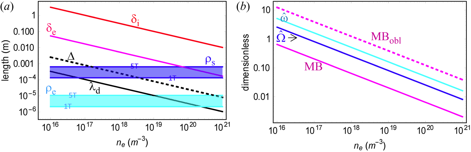
Figure 2. (a) Characteristic length scales and (b) dimensionless sheath parameters for a range of densities that might be encountered in fusion devices. See Appendix A for definitions. The importance of these characteristic scales and dimensionless parameters will become apparent later in the paper. In (a) the results for ρs and ρe are shown by the semi-transparent colours for magnetic fields between B = 1 T and 5 T. In (b) the Maxwell–Boltzmann ratio, $\textrm{MB} = \omega \Delta /({b_n}{v_{te}})$ , is shown at B = 5 T for normal incidence (solid) and for 3° grazing incidence (dashed). Further discussion of the MB ratio is given in § 4.3.2. Fixed parameters for this figure are $\omega = 2{\varOmega _i}$
 , ${T_e} = 20\;\textrm{eV}$
 , ${\varPhi _{\textrm{sh}}} = 300\;\textrm{V}$
 , deuterium plasma and here $\hat{\Omega } = {\Omega _i}/{\omega _{pi}},\;\hat{\omega } = \omega /{\omega _{pi}}$
 .
.
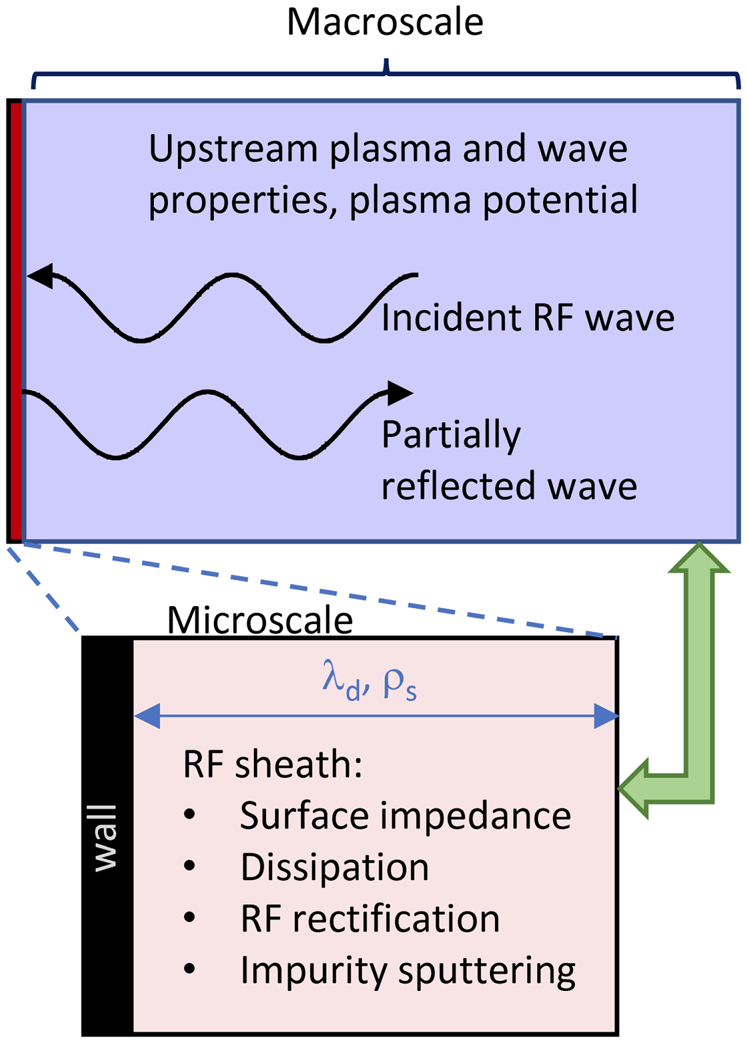
Figure 3. Schematic diagram showing interaction of microscale and macroscale sheath physics. The thick green arrow signifies the mutual coupling between these two scales.
The goal of microscale modelling is to calculate an effective surface impedance for the RF waves, RF sheath power dissipation and the rectified sheath potential. The macroscale and microscale are coupled because the RF sheath properties on the microscale depend on the RF wave amplitude at the sheath interface, determined by the macroscale model. On the other hand, the macroscale modelling depends on the sheath properties which set an effective boundary condition for the waves. On the macroscale the goal is to understand how the presence of an RF sheath modifies the wave, e.g. through reflection or absorption at the sheath interface, and how it modifies the plasma, e.g. as we will see, through the sheath-mediated generation of DC potentials that extend into the bulk plasma. This and several additional macroscale-related topics are discussed in § 6 followed by a concluding § 7. Tables of notations and acronyms are given in the Appendices.
2. Basic concepts
2.1. Static sheaths
Before proceeding to the main topic of RF sheaths, it is useful to briefly review the basic concepts governing static sheaths, since many of these concepts carry forward. The discussion that follows is elementary but sufficient for present purposes.
2.1.1. Basic perpendicular sheaths
When a plasma contacts a conducting wall, the thermal motion of the electrons and ions will cause those particles to impact the wall, resulting in plasma loss. Because electrons have larger speeds, they are initially lost more rapidly. This causes the plasma to develop a net positive potential with respect to the wall, of order a few times the electron temperature Te. The potential confines most of the electrons, i.e. those in the bulk of the distribution, by reflecting them back into the plasma. Furthermore, the electrical conductivity of plasma (in the absence of a magnetic field or parallel to it) is very good, so the electric field parallel to the background magnetic field in the plasma must be small, and hence the potential gradient required to confine the electrons cannot appear in the bulk plasma; instead, it is concentrated within a few Debye lengths λd of the wall where large electric fields are allowed because quasi-neutrality is broken, as shown in figure 4. In this Debye sheath layer electrons are largely excluded, having been reflected by the potential, and net positive ion charge supports the electric field. Plasma continues to flow to the wall but is limited by the speed at which ions can be removed. According to the Bohm sheath criterion (Stangeby Reference Stangeby2000), this speed must be at least the sound speed ${c_s} = {({T_e}/{m_i})^{1/2}}$ where mi is the ion mass. (For simplicity, a cold ion, isothermal electron model is considered here.Footnote 3 Thermal and kinetic ion effects will be discussed briefly in § 4.3.1.)
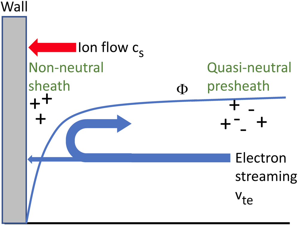
Figure 4. Schematic diagram illustrating the fundamental structure of a static unmagnetized sheath.
A source is required to sustain the plasma. Generally, the flow velocity of plasma at the source will be smaller than cs. A weak potential drop, about 0.7 Te develops over long scales in this source presheath region (Tonks & Langmuir Reference Tonks and Langmuir1929) to accelerate ions to the Bohm velocity cs at the entrance to the non-neutral sheath.Footnote 4 Since RF sheaths will typically be associated with much larger changes in potential, the source presheath region will not be of great concern in this paper.
The discussion just given is a greatly oversimplified description of the static sheath in an unmagnetized plasma. It also applies to a static sheath when the magnetic field is parallel or anti-parallel to the surface normal, i.e. perpendicular to the surface. (Caution: some authors refer to this geometry as a parallel sheath geometry; however, in this paper the opposite convention is followed, denoting it as a perpendicular geometry.) Thus, the term ‘unmagnetized sheath’ applies both to perpendicular magnetic field geometry as well as to the case when there is no magnetic field. The features just described are illustrated schematically in figure 4. The reader is referred to (Stangeby Reference Stangeby2000) for a more comprehensive treatment of static sheaths in magnetic fusion devices and also to (Hershkowitz Reference Hershkowitz2005) for an introduction to electron rich sheaths, probes, double layers, collisions and multiple ion species effects.
2.1.2. Biased sheaths
The preceding remarks apply to static sheaths that do not draw any net current or have any external voltage bias applied to them. If there is an applied potential difference between the plasma and the wall, the sheath must expand, thereby accommodating more charge to support the potential difference. It will be seen later that RF fields naturally apply a positive voltage to the plasma with respect to the wall. Here, we consider a positively applied DC bias to a perpendicular static sheath.
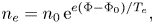
Employing the cold-ion model, at the entrance to the non-neutral sheath where the Bohm condition is met and the quasi-neutral density is n 0, the ion flux is n 0cs. The electron flux is obtained from the velocity moment of a Maxwellian retaining only those electrons in the tail of the distribution that have enough energy to escape the potential barrier presented by the sheath. The result is

where Φ 0 is the potential at the sheath entrance and v 0 is the electron escape velocity at the upstream location, defined by ${m_e}v_0^2/2 \equiv e({\varPhi _0}\; - {\varPhi _w})$ . If the conducting wall is grounded, Φw = 0, and connected to an external circuit, in general a current density J will flow into the wall
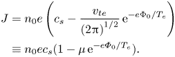
This is the textbook current–voltage characteristic for a sheath. The zero-current condition results in ${\varPhi _0} = \textrm{(}{T_e}/e\textrm{)ln}\mu$ where $\mu = {v_{te}}\textrm{/}[(2{\rm \pi} )^{1/2}{c_s}] = {[{m_i}/(2{\rm \pi} {m_e})]^{1/2}} = 24.17$
 for deuterium and ln μ = 3.18. A plot of normalized current vs. voltage is shown in figure 5.
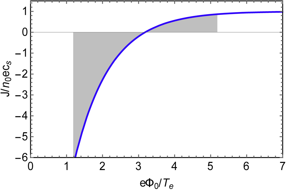
Figure 5. The current–voltage relation, (2.2) for a deuterium plasma (solid blue). The grey shaded area indicates the ranges of currents and voltages that would be sampled for a sinusoidal voltage oscillation of amplitude 2 about the zero-current point at $e{\varPhi _0}/{T_e} = 3.18$ . In this case net negative current would flow. This point will be returned to in § 2.2.
The internal structure of the non-neutral sheath is determined from Poisson's equation combined with a model for the electron and ion densities. Since the ions are the species flowing to the wall, the fluid model is the simplest, whereas the electrons, being the reflected species, may be taken as Maxwell–Boltzmann. The resulting equations in the sheath region are
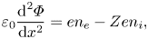

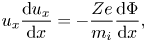
where the x coordinate is normal to the wall, the magnetic field is zero or in the ex direction and it is assumed that there are no particle sources in the sheath region.
From (2.5), integrating from the sheath entrance, ${n_i} = {n_0}{c_s}/{u_x}$ and from (2.6) $u_x^2 = c_s^2 + 2Ze({\varPhi _0} - \varPhi )/{m_i}$
 . The function ni(Φ) so obtained, ${n_i}(\varPhi ) = {n_0}{c_s}/[c_s^2 + 2Ze ({\varPhi _0} - \varPhi )/{m_i}]^{1/2}$
 and ne(Φ) from (2.4) may be substituted into (2.3) to obtain a nonlinear equation for the structure of the potential in the sheath. For the present purposes, an estimate of the sheath width will suffice. For a strongly biased sheath, i.e. $e{\varPhi _0}/{T_e} \gg 3.18$
 , the electron density in the sheath is nearly zero. From the preceding, the ion speed is of order ${u_x}\sim {(2Ze{\varPhi _0}/{m_i})^{1/2}}$
 and thus the ion density scales as ${n_i}\sim {n_0}{c_s}{[{m_i}/(2Ze{\varPhi _0})]^{1/2}}$
 in the large Φ 0 limit. The sheath width is therefore estimated from (2.3) by balancing the left-hand side, ${\varepsilon _0}{\varPhi _0}/{\Delta ^2}$
 , with the right-hand side, Zeni, to obtain $\Delta \sim {[{\varepsilon _0}{\varPhi _0}/(Ze{n_i})]^{1/2}}$
 or, neglecting the order-unity factor (2/Z)1/4
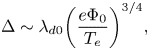
where the reference (sheath entrance) Debye length is $\lambda_{d0} = {[{\varepsilon _0}{T_e}/({n_0}{e^2})]^{1/2}}$ . Equation (2.7) is the well-known Child–Langmuir scaling. The sheath width will play an important role for RF sheath capacitive effects introduced in § 2.2.
2.1.3. Magnetized oblique sheaths
When a background magnetic field B exists and makes an oblique angle with the surface, the Lorentz u × B force is no longer negligible in the sheath dynamics. Its effect will depend on the ordering of scale lengths perpendicular to B. The most frequently encountered ordering in fusion plasmas, and the one considered in this article is ${\rho _e} \ll {\lambda _d}\sim {\rho _s} \ll {L_ \bot }$ , where ${\rho _e} = {v_{te}}/{\varOmega _e}$
 and ${\rho _s} = {c_s}/{\varOmega _i}$
 are the thermal electron and ion sound gyro-radiiFootnote 5 respectively, λd is the Debye length and L ⊥ is a characteristic macroscopic perpendicular scale length such as provided by device or wall geometry or the RF perpendicular wavelength. An important dimensionless parameter is the ion magnetization parameter in the sheath ${\rho _s}/{\lambda _d} = {\omega _{pi}}/{\varOmega _i}$
 . Here, ${v_{te}} = {({T_e}/{m_e})^{1/2}}$
 is the electron thermal velocity, ${\varOmega _i} = ZeB/{m_i}$
 and ${\varOmega _e} = eB/{m_e}$
 are the ion and electron cyclotron frequencies and ${\omega _{pi}} = {[{n_i}{Z^2}{e^2}/({\varepsilon _0}{m_i})]^{1/2}}$
 is the ion plasma frequency; Z is the ion charge and, in this discussion, we assume quasi-neutrality and Z = 1. See figure 2 for a comparison of some of these important scale lengths.
When both electrons and ions are strongly magnetized, ${\rho _e} \ll {\rho _s} \ll {\lambda _d} \ll {L_ \bot }$ their motion across the presheath and sheath regions is constrained to be parallel to the magnetic field, like beads on a string. The magnetic field enters only in so far as its orientation determines the projection of distances and velocities normal to the surface. See figure 6(a). In this limit, the structure of the sheath is formally analogous to an unmagnetized sheath.

Figure 6. Schematic diagram illustrating the fundamental structure of a static magnetized sheath in (a) the strongly magnetized ion regime, and (b) the weakly magnetized ion regime. In (b) the electrons are not shown for simplicity: they follow the same dynamics as in (a). The physics is unchanged if the magnetic field is anti-parallel instead of parallel to the upstream ion flow; the latter is always towards the surface.
In practice, the unmagnetized ion (in the sheath) regime is usually more relevant in fusion devices, ${\rho _e} \ll {\lambda _d} \ll {\rho _s} \ll {L_ \bot }$ . See figure 2(a). In the plasma region upstream of the sheath, the Debye scale is no longer present; the electric field is weak because L ⊥ is large, and therefore both electrons and ions are strongly magnetized, ${\rho _j} \ll {L _ \bot }(\kern0.06em j = e,i)$
 . In the upstream region, both species are constrained to follow magnetic field lines. Far upstream there is still a source presheath that accelerates ions from the source velocity to u = u ||b = ±csb, where b = B/B; see figure 6(b). A few Debye lengths from the wall, where a strong electric field exists in the non-neutral sheath region, the electric force ZeE dominates the magnetic force and ions are pulled across field lines into the wall. In the region between the non-neutral sheath and source presheath, there is a third region, the magnetic presheath, which has the job of accelerating ions from u || ~ cs (at the magnetic presheath entrance) to un ~ cs (at the non-neutral sheath entrance) where un = u⋅ n and n is the unit normal to the surface. This ensures that the Bohm condition, |un| ≥ cs, is met, and requires the establishment of a weak magnetic presheath electric field. Assuming that there are no particle sources in the magnetic presheath region, and noting that the ions are accelerated from un ~ cs sin θ to un ~ cs, it follows from conservation of flux, Γn = niun that ni must drop as one approaches the non-neutral sheath entrance. The magnetic presheath is still quasi-neutral (as allowed by the bulk plasma equations until |un| ≥ cs). As a result, the drop in ni also implies a corresponding drop in ne. This change in density tends to broaden the width (~λd) of the non-neutral sheath, which will have consequences for the RF interaction.
In the non-neutral sheath itself, the force on the ions from the electric field is dominant and therefore the sheath ions are not strongly magnetized. Specifically, estimating $E\sim \varPhi /{\lambda _d}\sim {T_e}/(e{\lambda _d})$ and for the ions u × B ~ csB results in $E/|\boldsymbol{u} \times \boldsymbol{B}|\sim {\rho _s}/{\lambda _d} \gg 1$
 by assumption. On the other hand, the electrons are still strongly magnetized in the sheath: since u ~ vte, the ratio of electric to magnetic force for the electrons is of order ${\rho _e}/{\lambda _d} \ll 1$
 by assumption.
The oblique magnetized sheath is a complicated object, only described at the most basic level here, concentrating on the aspects that will be most important for RF sheaths. A more comprehensive treatment of magnetized sheaths has been given in Daybelge & Bein (Reference Daybelge and Bein1981) and Chodura (Reference Chodura1982) and some additional subtleties are discussed in Cohen & Ryutov (Reference Cohen and Ryutov1995). One important point is that standard sheath theories assume that b⋅ n is not too small; otherwise, the electrons which are constrained to follow field lines, are better confined than the ions. This point will be returned to in § 6.9.
Finally, it is not difficult to generalize the discussion of biased perpendicular sheaths to that of an oblique magnetized sheath; a detailed treatment will be deferred to the RF case. Suffice it to note that when a magnetized sheath is biased, most of the voltage drop must appear across the non-neutral sheath because extra (un-neutralized) charge is required there to balance the extra potential, just as in § 2.1.2. The main difference that an oblique magnetic field introduces is that the quasi-neutral density drops throughout the magnetic presheath. This makes the density at the entrance to the non-neutral sheath smaller than the upstream density, and thereby increases the effective Debye length and the sheath width.
2.1.4. More sophisticated models
Before closing this short section on static sheaths, it should be noted that many more sophisticated models have been developed and studied to take into account effects such as secondary electron emission (Stangeby Reference Stangeby2000; Campanell & Umansky Reference Campanell and Umansky2017), non-Maxwellian electron distributions (Ou et al. Reference Ou, Lin, Zhao and Yang2016), collisions (Tang & Guo Reference Tang and Guo2015), ionization and kinetic ion effects (Khaziev & Curreli Reference Khaziev and Curreli2015) and E × B and diamagnetic drifts (Cohen & Ryutov Reference Cohen and Ryutov1999; Stangeby Reference Stangeby2000). These are but a few of the many hundreds of papers in the literature on these and related topics. Some of the mentioned effects are not usually of prime importance for the RF sheaths of interest in tokamak heating and current-drive experiments (which is not to discount their importance for static sheaths in the divertor where neutral physics, grazing angle magnetic geometry and cool, dense, more collisional plasmas can prevail). Other effects remain to be studied in the RF context. RF sheath studies for fusion research have up until recently been occupied with more fundamental (i.e. zero-order) effects, namely those which are essential for coupling sheath physics to global RF wave propagation codes and impurity codes. A brief treatment of secondary electron emission is included in the considerations of § 6.3.
2.2. Rectification and sheath impedance: capacitive RF sheaths
The simplest and probably most widely studied RF sheath is the capacitive sheath. It serves as a good introduction to the topics of rectification and sheath impedance (or its reciprocal, sheath admittance) which will be treated in more detail in subsequent sections. A capacitive sheath is so named because the displacement current dominates the particle currents flowing across the sheath. It will be shown in § 4 that this limit occurs at high frequency, $\omega \gg {\omega _{pi}}$ where ωpi is the ion plasma frequency. A rough idea for the cases when this condition is fulfilled may be gleaned from figure 2. At the location of the antenna the RF wave frequency is usually somewhat larger than the local ion cyclotron frequency. In figure 2 the value of $\hat{\omega } = \omega /{\omega _{pi}}$
 for $\omega = 2{\varOmega _i}$
 is shown as a function of density for a high-field device, B = 5 T. At low sheath entrance densities, the high-frequency condition can be satisfied.
Consider the case of a plasma-filled region between two parallel plates, with surface normal n and background magnetic field B normal to the surface as shown in figure 7(a). Let the plates be driven by anti-symmetric voltages on each side, namely ${V_1} ={-} {\varPhi _{rf}}\cos \omega t$ , ${V_2} ={-} {V_1}$
 and consider the plasma potential Φ 0 in the centre of the device, far away from the plates and their associated sheaths. This will be referred to as an anti-symmetric sheath (model). Although the DC voltage on both plates is zero, it can readily be seen that Φ 0 can acquire a DC voltage much greater than 3.18 Te when the driving voltage Φrf is large.

Figure 7. (a) Geometry of a double-plate capacitive sheath model with anti-symmetric RF voltage source. (b) Sketch of the corresponding potential in the plasma at three different times in the RF cycle. (c) Sketch of the RF potentials near the left plate with zero potential at the plate. Here, the illustration corresponds to the average Δ model for sheath capacitance.
The electrostatic potential Φ(x) is sketched in figure 7(b) for three different times during the RF cycle, $\omega t = 0$ , ${\rm \pi} /2$
 and ${\rm \pi}$
 . Note the changes in potential drop across each sheath and the corresponding expansion and contraction of the sheath width according to the Child–Langmuir scaling of (2.7). At each instant of time, assuming a Maxwell–Boltzmann (and hence instantaneous) response for the electrons, Φ(x) in the bulk plasma must remain 3.18 Te above the instantaneous voltage at either plate; otherwise, the electron current losses would greatly exceed the ion current losses and the bulk plasma could no longer remain quasi-neutral. The electric field in the middle of the domain is negligible compared with that in the sheaths because the plasma electrical conductivity along the magnetic field is very high. (Furthermore, for simplicity we assume in this example that no net DC current is allowed to flow from one plate to the other.) It is evident that the DC or average upstream potential $\langle {\varPhi _0}\rangle$
 measured in the centre of the domain, exhibits ‘rectification’ of the applied RF voltage. The 3.18 Te static sheath potential is still present and additive with the RF rectification effect.Footnote 6
Numerical simulations and analytic theory (Lieberman Reference Lieberman1988; Godyak & Sternberg Reference Godyak and Sternberg1990; Myra et al. Reference Myra, D'Ippolito and Gerver1990) show that for $e{\varPhi _{rf}} \gg {T_e}$ the rectified potential $\langle {\varPhi _0}\rangle$
 increases approximately linearly with the RF voltage $\langle {\varPhi _0}\rangle \sim {C_0}$
 Φrf with C 0 a constant of order 0.6; at low voltages $e{\varPhi _{rf}} \ll {T_e}$
 , of course one recovers the static sheath result $e\langle {\varPhi _0}\rangle = {T_e}\ln \mu \sim 3.18 \hspace{0.1 cm} {T_e}$
 . These behaviours are illustrated in figure 8.
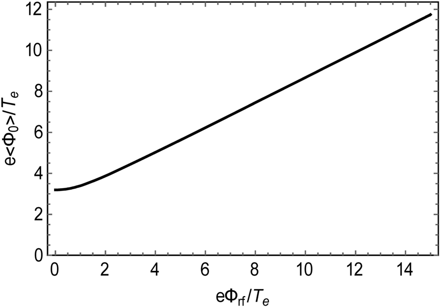
Figure 8. Typical variation of the DC plasma potential in a deuterium plasma as the driving RF plasma potential is changed.
Voltage rectification occurs in this example partly because the net DC current is constrained to be zero. Another way of understanding rectification is by referring to figure 5. It can be seen that, for a single-ended sheath, the zero-current condition (equal positive and negative shaded areas) would require the voltage oscillation to be centred at a higher value than the 3.18 Te value illustrated in the figure. Conversely, if the external circuit prevents voltage rectification, the asymmetry of the current–voltage relation leads to current rectification as illustrated by the net negative shaded area in figure 5.
The capacitive property of the sheath has not yet played a significant role in the discussion. In fact, the cartoon sketches in figure 7 would not be different if the plates were statically biased. The capacitive property enters when the sheath impedance is considered. The sheath impedance is a convenient way to characterize how the presence of the sheath affects RF wave fields that are in contact with the sheath surface. A more sophisticated calculation of the sheath impedance will be discussed in § 4; here, a semi-heuristic intuitive approach is given for the high-frequency capacitive limit.
In practice, the sheath width is almost always very small compared with characteristic scales along the surface (geometric, RF wavelengths and the vacuum wavelength c/ω). This makes the sheath problem one-dimensional with the electric field normal to the surface Ex a function of x (locally on the scale of the sheath) and therefore electrostatic, $\boldsymbol{\nabla } \times {\boldsymbol{E}_x}(x) = 0$ . In electrostatic theory one can add an arbitrary time-dependent but spatially constant function to the potential without changing the physical observables. To analyse the impedance, it is simplest to consider the sheath on the left of figure 7 with the potential shifted so that the wall is at ground and the applied oscillation is in the bulk upstream plasma, as if supplied by an RF wave. The corresponding potential for three different RF phases, ωt = 0, ${\rm \pi}$
 /2 and ${\rm \pi}$
 , are sketched in figure 7(c).
Electrons are mostly excluded from the non-neutral sheath, 0 < x < Δ, having been reflected by the sheath potential. Ions are present, but in the high-frequency limit, $\omega \gg {\omega _{pi}}$ , inertia prevents them from responding directly to the RF wave. (In the literature, this high-frequency limit is sometimes referred to as the ‘immobile’ ion limit where the immobility applies at the RF frequency.) As a result, as far as the RF waves are concerned, the sheath behaves like a vacuum gap of average width Δ, where Δ is determined from the rectified potential by (2.7).Footnote 7 Within this simple model, the effect of the sheath on the RF wave fields may be determined by matching the RF fields across this narrow vacuum layer before applying the usual conducting wall boundary condition at the actual plate location (D'Ippolito & Myra Reference D'Ippolito and Myra2006).
The matching condition at the sheath–plasma interface is the continuity of the surface normal component n of displacement $\boldsymbol{D} = {\varepsilon _0}\boldsymbol{\varepsilon }\boldsymbol{\cdot }\boldsymbol{E}$ where $\boldsymbol{\varepsilon }$
 is the relative permittivity tensor of the plasma or vacuum region. For the ‘perpendicular’ sheath problem considered at present, this reduces to the matching condition ${E_{x,\textrm{vac}}} = {\varepsilon _{||}}{E_{x,\textrm{pl}}}$
 where ‘vac’ indicates the vacuum gap (sheath) region and ‘pl’ is the plasma region (at the sheath entrance). See figure 7(c). Since $|{\varepsilon _{||}}|= |1 - \omega _{\textrm{pe}}^2/{\omega ^2}|\gg 1$
 is large in the ICRF frequency regime, this results in very large electric fields in the sheath region, ${E_{x,\textrm{vac}}} ={-} \partial \varPhi /\partial x$
 . In this simple model, since the vacuum layer is uniform, Φ varies linearly from zero at the conducting wall to a finite value at the vacuum– (i.e. sheath–) plasma interface. The RF sheath voltage at the interface is therefore
where n is the direction of the outward surface normal (ex at the left plate). Furthermore, along the vacuum–plasma interface of the sheath, the RF tangential electric field Et must be the negative tangential gradient of the RF sheath potential. The sheath boundary condition, may therefore be expressed as the continuity of Et, i.e.
Equation (2.9) expresses the capacitive sheath boundary condition (BC) for a perpendicular sheath entirely in terms of RF field quantities on the plasma side of the sheath, as required for a BC.
Finally, the right-hand side of (2.8) is proportional to the plasma current density ${J_n} = {\sigma _{||}}{E_n}$ where ${\sigma _{||}} ={-} \textrm{i}\omega {\varepsilon _0}{\varepsilon _{||}}$
 . Here, and throughout whenever complex notation is employed, the exp(−iωt) phase convention is assumed. Consequently (2.8) takes the form
where z sh, being the ratio of a voltage and a current per unit area is identified as the sheath impedance parameter. (Note the minus sign: the impedance is calculated from the drop in voltage in the direction of the current, Jn.) Its reciprocal y sh = 1/z sh is the sheath admittance per unit area. In the final form of (2.11), $C^{\prime} = {\varepsilon _0}/\Delta$ is the sheath capacitance per unit area.
Equation (2.10) suggests a general way of expressing the sheath BC. First, from a general microscale model of the sheath, the RF current passing through the sheath Jn (retaining electron, ion and displacement currents) is determined in terms of the voltage across the sheath Φ sh. This defines the sheath impedance z sh. Then the corresponding BC for a sheath on a perfectly conducting surface is given by
where here, and in future discussions of the sheath BC, the subscript ‘pl’ is dropped: all RF field quantities in the sheath BC are assumed to be evaluated on the (upstream) plasma side of the sheath. The evaluations of z sh, Φ sh and the use of the sheath BC in more general settings are the subject of §§ 4–6.
3. RF sheath classification in fusion devices
The particular geometry, hardware (i.e. launchers, limiters and device walls) and wave scenarios encountered in fusion devices allow various types of RF sheaths to exist. Here, the discussion is mainly written with ICRF sheaths in mind, since experimental observations in the ICRF regime motivate the classification. Furthermore, unless otherwise stated, ‘sheath’ should be assumed to refer to an RF sheath.
RF sheaths in fusion devices differ by their location, magnetic connection (or not) to an antenna or launcher, whether they are driven by near fields or propagating waves, and if the latter, the polarization of those waves. These considerations are at least conceptually separate from the dimensionless parameters that characterize the physical regime of the sheath, to be introduced in (4.11a–e), although in practice they may be linked. In the following subsections, some commonly encountered types of sheaths are described with the goal of providing real-world context for the more physics-based discussions of sheath models which follow. The rough categorization of sheaths into these distinct types is conceptually useful to illustrate different mechanisms, which is not to say that the mechanisms are mutually exclusive.
3.1. Near-field antenna sheaths
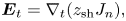
When a magnetic field line makes a connection between two points on the surface of an antenna or its nearby hardware, high-voltage sheaths can form, which are driven directly by the applied RF voltages and currents and their near fields. An example is illustrated in figure 9(a). Contact points on the Faraday screen bars, side limiters and septa often result in magnetic connections subject to high RF driving voltages associated with the encircled RF magnetic flux (Bures et al. Reference Bures, Jacquinot, Lawson, Stamp, Summers, D'Ippolito and Myra1991). As a rough order of magnitude estimate, the sheath voltage Φ sh can be as large as a fraction f of the top-to-bottom antenna voltage Φ sh = fV ant where f = Lc/La is given by the ratio of poloidal distance subtended by the field line between contact points, Lc, and the top-to-bottom poloidal antenna dimension, La. See figure 9.
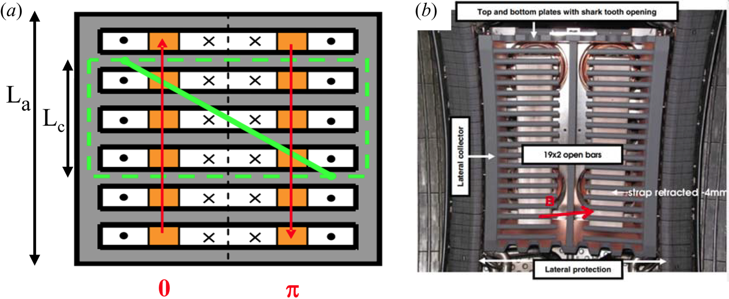
Figure 9. (a) Sketch of near-field antenna sheath geometry showing a magnetic field line (solid green), its contact points and the flux loop path completed through the antenna frame (dashed green). Here, 0 and ${\rm \pi}$ indicate relative phasing of the antenna strap currents. Solid black dots and crosses indicate the direction (respectively out of and into the page) of the RF magnetic field. For a symmetric sheath in dipole phasing (antenna strap currents shown with red arrows) there is RF magnetic flux cancellation and no induced voltage between symmetrical contact points. In monopole phasing (0–0, not illustrated) the voltages can be very large. The poloidal distances La and Lc mentioned in the text are shown at left. (b) Photograph of one of the ICRF antennas from the Tore Supra device. This particular antenna features cantilevered bars, a central septum and a slotted box. Reprinted by permission from figure 2(b) of Corre et al. (Reference Corre, Firdaouss, Colas, Argouarch, Guilhem, Gunn, Hamlyn-Harris, Jacquot, Kubic, Litaudon, Missirlian, Richou, Ritz, Serret and Vulliez2012).
The actual sheath voltage depends on many design factors (as well as plasma factors discussed in the rest of this paper) and considerable effort has been made in the RF fusion community to mitigate sheath interactions by careful antenna engineering and operation. A complete discussion of these techniques is beyond the scope of this paper. Suffice it to say that important considerations are: antenna phasing (D'Ippolito et al. Reference D'Ippolito, Myra, Bures and Jacquinot1991; Bures et al. Reference Bures, Jacquinot, Stamp, Summers, Start, Wade, D'Ippolito and Myra1992) and relative powering of different straps (Bobkov et al. Reference Bobkov, Braun, Dux, Herrmann, Faugel, Fünfgelder, Kallenbach, Neu, Noterdaeme, Ochoukov, Pütterich, Tuccilo, Tudisco, Wang and Yang2016, Reference Bobkov, Aguiam, Bilato, Brezinsek, Colas, Faugel, Fünfgelder, Herrmann, Jacquot, Kallenbach and Milanesio2017a) in multi-strap designs; orientation of the antenna with respect to the direction of the magnetic field (Wukitch et al. Reference Wukitch, Garrett, Ochoukov, Terry and Hubbard2013); control of induced currents in the antenna frame and sidewalls (Bobkov et al. Reference Bobkov, Balden, Bilato, Braun, Dux, Herrmann, Faugel, Fünfgelder and Giannone2013), the reduction of RF electric fields parallel to B (Tierens et al. Reference Tierens, Jacquot, Bobkov, Noterdaeme and Colas2017) and the use of insulating coatings (Majeski et al. Reference Majeski, Probert, Tanaka, Diebold, Breun, Doczy, Fonck, Hershkowitz, Intrator, McKee, Nonn, Pew and Sorensen1994). The physics of the latter is discussed in § 6.9. The other strategies involve RF engineering issues best addressed with electromagnetic simulation codes. Work is ongoing to implement a sheath BC into these codes to allow for a self-consistent response of the RF simulations to the sheath, and to provide a predictive capability for the sheath voltages and the resulting plasma–material interactions such as sputtering.
3.2. Magnetically connected far-field sheaths
A second type of sheath occurs when a magnetic field line on a surface far away from the antenna is magnetically connected to a point on the antenna. The far surface could be a distant limiter, divertor structure, the inner wall or another piece of hardware intruding into the scrape-off layer (SOL). In this case the magnetic connection to the antenna can be important for both the RF and DC potentials that appear at the remote location. RF waves excited at the antenna that propagate mostly along the magnetic field can generate a far-field RF sheath on the remote surface. For ICRF waves, (Stix Reference Stix1992) the slow wave (SW) fits into that category and also has the correct polarization (§ 3.4) for a strong RF sheath interaction. An example of a magnetically connected sheath is illustrated in figure 10(b) which shows a curved model antenna at right that magnetically connects to the vessel wall at bottom. This figure shows filled contours of E || which is a proxy for the SW. Note that the SW generated at the antenna propagates along the magnetic field, i.e. along the flux surfaces in this R–Z plane cut of the torus.
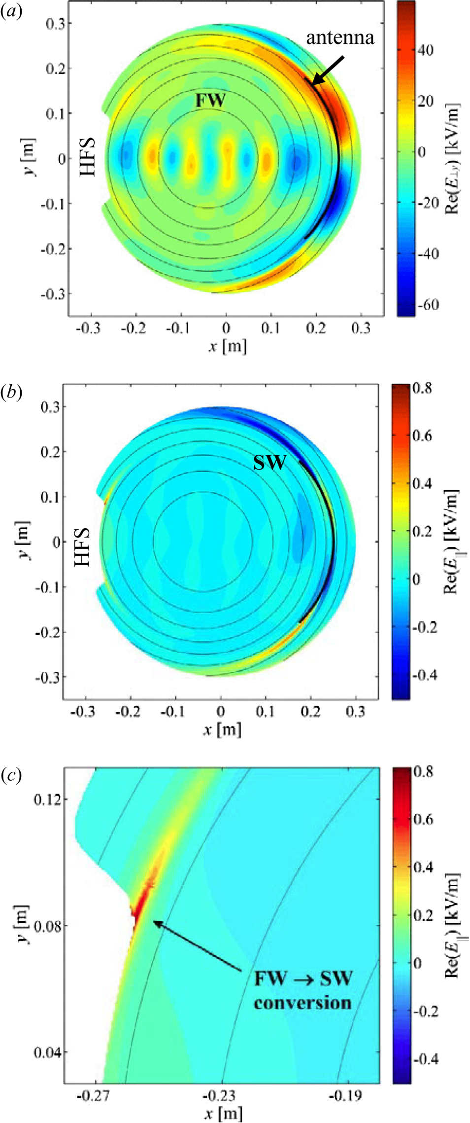
Figure 10. Far-field sheath simulation results in the R–Z plane (shown here as x–y) of a tokamak in a model geometry: (a) filled contours of Re(E ⊥) showing unabsorbed FWs striking the high-field sidewall; (b) filled contours of Re(E ||); and (c) an expanded view of Re(E ||) near a limiter protrusion on the high-field side. The light-coloured concentric circles are magnetic flux surfaces and the thick black curved structure at right is a model antenna. The high-field side (HFS) of the torus is at left. Reprinted by permission from figure 3 of Kohno (2016).
Although modern antennas for fusion research devices are almost always designed to launch the fast wave (FW) some parasitic coupling to the SW is unavoidable. The SW is associated with parallel currents and electric fields, and can be minimized by aligning active current elements in the antenna structure to be perpendicular to the background magnetic field, as explored experimentally in Alcator C-Mod (Wukitch et al. Reference Wukitch, Garrett, Ochoukov, Terry and Hubbard2013). Here, and throughout this paper, ‘parallel’ without other qualifiers means parallel to the background magnetic field.
In a magnetically connected propagating SW scenario, the RF wave at the remote surface will generate a local rectified (DC) sheath potential (Myra & D'Ippolito Reference Myra and D'Ippolito2008), analogous to the mechanism discussed in § 2. But there are other factors, which influence the DC sheath potential. In particular, if there is good DC electrical conductivity between the antenna sheath contact point and the magnetically connected far-field sheath, the antenna sheath which is generally stronger may dominate the DC sheath potential at the remote location (Lu et al. Reference Lu, Colas, Jacquot, Després, Heuraux, Faudot, Van Eester, Crombé, Křivská, Noterdaeme, Helou and Hillair2018; Myra et al. Reference Myra, Lau, Van Compernolle, Vincena and Wright2020). Also, to the extent permitted by finite DC resistivity, a DC potential difference may be established between the antenna sheath and the far-field sheath governed in part by the DC plasma current which will flow between these two surfaces. DC currents associated with applied ICRF power have been observed in many experiments (Van Nieuwenhove & Oost Reference Van Nieuwenhove and Oost1992; Bobkov et al. Reference Bobkov, Bilato, Colas, Dux, Faudot, Faugel, Fünfgelder, Albrecht and Jonathan2017b; Perkins et al. Reference Perkins, Hosea, Jaworski, Bell, Bertelli, Kramer, Roquemore, Taylor and Wilson2017, Reference Perkins, Hosea, Taylor, Bertelli, Kramer, Luo, Qin, Wang, Xu and Zhang2019; Myra et al. Reference Myra, Lau, Van Compernolle, Vincena and Wright2020). DC current flow will be discussed in more detail in § 6.6. This type of situation is often referred to as an asymmetric RF sheath, in contrast to the anti-symmetric model illustrated in figure 7.
From the microscopic point of view, both situations may be analysed in the framework of a local RF sheath model, as discussed in § 4, but one in which there may be an ‘external’ DC current flow and an ‘external’ DC voltage bias. The macroscopic problem (§ 6) has the task of relating sheaths, DC potentials and RF waves at various locations in the device to each other in a self-consistent way.
3.3. Not-magnetically connected far-field sheaths
A third type of sheath is the not-magnetically connected far-field sheath. This type of sheath occurs when a propagating wave strikes a remote surface that is not magnetically connected to an antenna or other active RF source. The distinction from the magnetically connected far-field sheath is particularly clear for ICRF waves because SW propagation is nearly along the magnetic field while FW propagation is to a much greater extent directed across the magnetic field. Thus, not-magnetically connected far-field ICRF sheaths are usually associated with a FW impinging on a wall or other surface. This could happen in two ways: (i) when FW antennas drive coaxial modes (Messiaen & Maquet Reference Messiaen and Maquet2020) i.e. surface waves and/or waves between the edge plasma and vessel wall, that propagate in the SOL around the torus poloidally (and toroidally), or (ii) when the central absorption of the FW is poor so that ‘shine through’ illuminates the inner wall or other surface.
An example of the latter case is illustrated in figure 10. Figure 10(a) shows filled contours of E ⊥ which, in the central plasma, is a proxy for the FW fields. FWs which are not absorbed in the core strike a limiter protrusion on the inner wall, at far left in the figure. At locations where the limiter surface is not coincident with a flux surface, i.e. where $|\boldsymbol{b}_p\boldsymbol{\cdot }\boldsymbol{n}|\ne 0$ , the BCs at the surface in general require both FW and SW components. Figure 10(c) shows filled contours of E || near the ‘corner’ of the limiter protrusion. At this location FW–SW coupling occurs and an RF sheath forms. The physics of this is discussed in § 3.4.
Usually there will be a FW cutoff on the high-field side of the torus beyond which the FW is evanescent. Thus, in the case of (ii) the distance between the cutoff and the wall in comparison with the evanescent decay length determines the strength of the FW–wall interaction. The evanescent decay length decreases with the FW parallel wavenumber, k ||, therefore the interaction is strongest for low k || waves. Not-magnetically connected sheaths have been documented in several experiments (Perkins et al. Reference Perkins, Hosea, Kramer, Ahn, Bell, Diallo, Gerhardt, Gray, Green and Jaeger2012; Ochoukov et al. Reference Ochoukov, Whyte, Brunner, D'Ippolito, LaBombard, Lipschultz, Myra, Terry and Wukitch2014).
3.4. Wave polarization: FW and SW interactions
For ICRF wave interactions, strong, i.e. high voltage, RF sheaths are usually associated with the presence of the SW. A heuristic way of understanding this is evident from (2.8) for perpendicular capacitive sheaths, which states that ${\Phi _{\textrm{sh}}} ={-} {\varepsilon _{||}}\mathrm{\Delta }{E_{n,\textrm{pl}}}$ . Even for rather low-density edge plasmas, the parallel dielectric, $|{\varepsilon _{||}}|= |1 - \omega _{\textrm{pe}}^2/{\omega ^2}|\gg 1$
 , is rather large. For example, at 50 MHz and a density of only 1017 m−3 we find ε || = −3200. The large value of ε || compensates for the inevitably small value of sheath width Δ, and makes a large sheath voltage Φ sh possible. The appearance of ε || in the expression for sheath voltage is directly associated with the presence of E || and the SW polarization.
More generally, the RF sheath voltage is given by (2.10), ${\Phi _{\textrm{sh}}} ={-} {z_{\textrm{sh}}}{J_n}$ . The normal component of the RF current is

where $\boldsymbol{\varepsilon }$ is the dielectric tensor, given in cold fluid theory by (Stix Reference Stix1992)

where $\boldsymbol{I}$ is the unit tensor, ${\varepsilon _ \bot } = 1 + \omega _{\textrm{pi}}^2/(\Omega _i^2 - {\omega ^2}),\;{\varepsilon _{||}} = 1 - \omega _{\textrm{pe}}^2/{\omega ^2}$
 and ${\varepsilon _ \times } = \omega _{\textrm{pi}}^2\omega /{\Omega _i}({\omega ^2} - \Omega _i^2)$
 . It can be seen that, unless E has a parallel component, ε || does not enter; instead, only the much smaller components ε ⊥ and ε × enter, and the resulting sheath voltage tends to be small.
Except under special circumstances, any BC will tend to couple various components of the electric field at the boundary. In general, it is not possible to satisfy a BC on the RF electric field E unless both FW and SW components are present. The sheath BC has this property of coupling the FW and SW, but in fact so does the perfectly conducting wall BC. The conducting wall limit will be used next to provide an example of how the SW can be generated at a boundary from a pure FW.
The geometry of the interaction is illustrated in figure 11. When the magnetic field is oriented obliquely with respect to the surface, it is apparent that the FW and SW are coupled by the BC. The FW electric field is (almost entirely) perpendicular to the background magnetic field B, but in order to make the tangential field Et zero on the surface, and hence the total field E = E⊥ + E|| purely normal to the surface, a finite E || is necessary. This implies a finite amplitude of the SW. Thus, a pure incoming FW will, in general, generate a SW and an E || by its interaction with the boundary. In two special cases the FW does not couple to a SW. If the magnetic field is ‘perpendicular’ to the surface, i.e. |b⋅n| = 1 an E || is allowed but is not needed. In this case a pure FW will simply arrange its phase such that Et is zero on the surface, i.e. the surface is a node of the oscillations. The second case is when the magnetic field is tangent to the surface, b⋅n = 0. Then E || is not required from consideration of the geometry. However, the case b⋅n = 0 is singular from the point of view of sheath theory, since electrons (ions) at a greater distance than ρe (ρi) from the wall cannot escape the plasma, at least not without invoking cross-field transport; see § 6.9.2.
Figure 11. Geometry of an oblique magnetic field RF interaction with a surface for which the perfectly conducting BC, Et = 0 has been applied. The FW electric field is polarized in the direction of E⊥. In order to satisfy the BC, an E || and hence a SW must be generated at the surface.
Although the preceding example is for the perfectly conducting wall BC, the conclusion about BCs coupling the FW and SW polarizations holds in general (non-pathological) cases. A more rigorous treatment is given in § 6.4.
4. Microscale RF sheath model
As discussed in the introduction, and summarized in figure 3, microscale models deal with the physics that occurs in the sheath itself, on the scale of a few Debye lengths for the non-neutral sheath, and on the ρs scale for the neutral magnetic presheath. The role of the microscale model is to input plasma density, temperature and DC current, magnetic field, geometric and RF parameters at the sheath–plasma interface (strictly speaking, at the entrance to the magnetic presheath) and from them calculate the DC plasma potential (i.e. RF rectification) and the RF surface impedance that the sheath presents to the RF wave fields in the bulk plasma. These output quantities are also computed at the sheath–plasma interface.
One can envision here a hierarchy of physical models capable of connecting the previously mentioned inputs and outputs. They may differ in the plasma description (fluid vs kinetic) and geometry (single-ended vs. double-plate RF excitation) or in other ways. The fluid model discussed first will provide a concrete example. Kinetic models currently under use will also be mentioned. Other models and embellishments are discussed at the end of this section.
4.1. RF sheaths in the nonlinear fluid (NoFlu) model
The capacitive sheath model introduced in § 2.2 is often a reasonable model for a low-density RF sheath satisfying ω > ωpi. It has been widely used in both the plasma processing and fusion communities. In the present section we consider the next level of sophistication by considering not only the displacement current flowing through the sheath, but also the particle currents. This requires a dynamical plasma model, provided here by the cold-ion fluid equations and a Maxwell–Boltzmann model for the electrons. This model will be referred to as the ‘NoFlu’ or ‘nonlinear fluid’ model. It is a time-dependent generalization of (2.3)–(2.6). The NoFlu model uses the same double-plate geometry as the capacitive sheath model, but with additional parameters. Labels and other, now relevant, details are shown in figure 12.
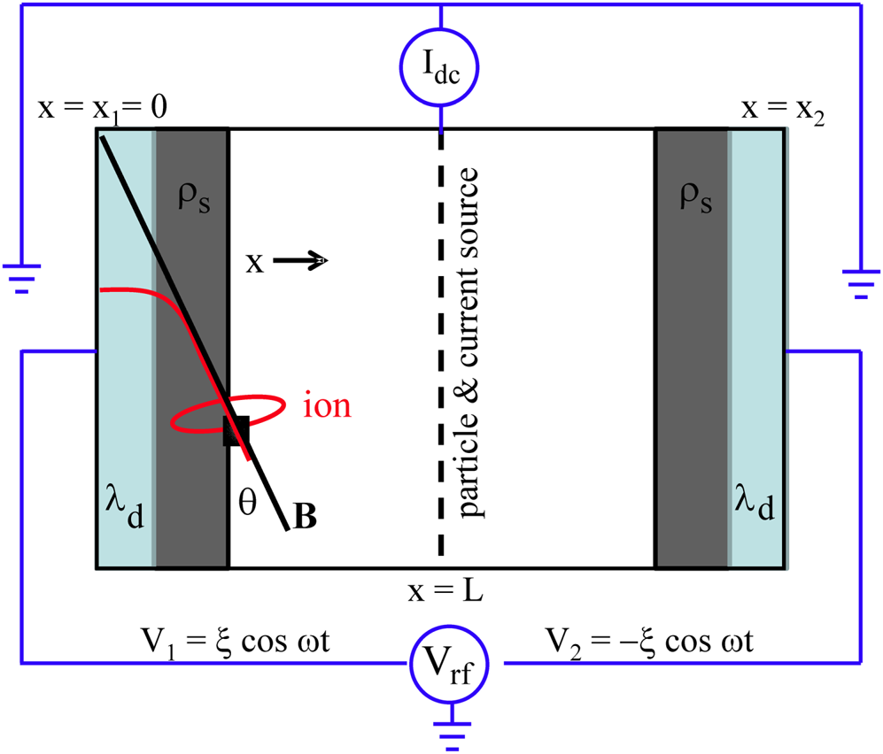
Figure 12. Anti-symmetrically driven double-plate RF sheath model. Plasma fills the interior region. The conducting plates are DC grounded and the RF voltage is driven ${\rm \pi}$ out of phase on each plate with normalized amplitude ξ. Particle and current sources are located at the midplane x = L. Reprinted by permission from figure 1 of Myra et al. (Reference Myra, Elias, Curreli and Jenkins2021).
4.1.1. Dimensionless variables and model equations
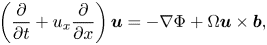
It is convenient to convert to dimensionless variables that are natural for this model: space scales normalized to the Debye length λd, time scales to the inverse ion plasma frequency 1/ωpi, the electrostatic potential to Te/e and currents to the ion saturation current ni 0ecs. Here, we restrict the discussion to singly charged ions and throughout this paper temperatures are expressed in units of energy. The ion velocity u is normalized to the cold-ion sound speed cs. The quantity ni 0 is the ion (or electron) density at the (quasi-neutral) entrance to the magnetic presheath, i.e. at the centre of the domain x = L in figure 12. Normalizing density to the density at the sheath entrance ni 0, the equations of the model are


where x is the spatial coordinate perpendicular to the plate, Φ(x,t) is the electrostatic potential, ni(x,t) and ne(x,t) are the electron and ion densities and ${\varPhi _0}(t) = \varPhi (L,t)$ is the central (upstream) potential. As before, b is the unit vector in the direction of the background magnetic field, and Ω is the dimensionless ion cyclotron frequency, parametrizing the degree of ion magnetization in the sheath.
The model has localized delta-function particle and current sources at the midplane x = L. These are implemented through the BCs and constraints as follows:


where L − (L +) signifies the value just to the left (right) of x = L.
The current conservation condition $\boldsymbol{\nabla }\boldsymbol{\cdot }({\boldsymbol{J}_d} + {\boldsymbol{J}_i} + {\boldsymbol{J}_e}) = 0$ provides an equation that determines Φ 0(t). (Recall that the continuity equation for each species (j = i, e) gives $\partial {\rho _j}/\partial t + \boldsymbol{\nabla }\boldsymbol{\cdot }{\boldsymbol{J}_j} = 0$
 and that the time derivative of the total charge ∂ρ/∂t is, from the time derivative of Poisson's equation, just ∇⋅Jd where ${\boldsymbol{J}_d} = {\varepsilon _0}\partial \boldsymbol{E}/\partial t$
 .) The current at the left plate is given by

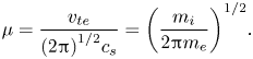
where subscript 1 indicates evaluation at x = x 1. Here, we expect ux 1 < 0 in the ion term (the first term), and the electron (i.e. second) term is in analogy to (2.2) where μ is defined by
By the symmetry of the problem, at the right plate ${J_{x2}}(\omega t) ={-} {J_{x1}}(\omega t + {\rm \pi})$ . The current conservation condition then becomes
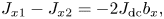
where J dc is the dimensionless injected DC current. Equation (4.10) determines Φ 0(t).
To complete the specification of the model, u0 must be given. A suitable choice is to take ${\boldsymbol{u}_0} = {u_{||0}}\boldsymbol{b}$ where $|{u_{||0}}|\ge {c_s}$
 , typically ${u_{||0}}/{c_s} ={-} 1.0$
 or in Myra (Reference Myra2017) ${u_{||0}}/{c_s} ={-} 1.1$
 . Results of interest are not very sensitive to these choices. The model is also well posed for $\textrm{|}{u_{||0}}\textrm{|} < {c_s}$
 but in that case a source-related presheath will form as reviewed in § 2.1. This presheath, not to be confused with the magnetic presheath (see figure 6b), is unrelated to the RF quantities of interest. It is best not modelled here because in a real plasma the presheath would extend over global scale lengths while we wish to model a sheath BC to be applied within a few ρs or λd lengths from the surface.
All of the output quantities of interest are functions of five dimensionless input parameters of the model

together with the auxiliary parameters $\mu = {[{m_i}/(2{\rm \pi} {m_e})]^{1/2}}$ and ${u_{||0}}/{c_s}$
 . In particular, the rectified voltage and sheath impedance are given by

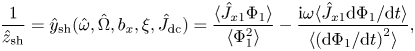
or equivalently

where, φ = ωt, the bracket notation $\langle \cdots \rangle = \int {\textrm{d}\varphi /(2{\rm \pi} ) \ldots }$ is used to indicate an average over a complete RF cycle and for extra clarity where confusion might occur the circumflex notation (super ^) is temporarily introduced to denote dimensionless variables. Equation (4.13) shows that the complex admittance is just the Fourier projection at frequency ω of the current flowing through the sheath for a given RF voltage drop across the sheath.
Numerical methods for solving the NoFlu model will not be discussed here in any detail except to mention two general approaches. The most direct approach is to integrate forward in time from an arbitrary initial condition, and continue time stepping until the system relaxes to an approximately periodic state with period 2${\rm \pi}$ /ω. Standard numerical techniques for computational fluid dynamics, such as upwind differencing or implicit time stepping may be required for numerical stability. A second technique is to discretize in both space and time, where the time discretization is over just one RF period and time periodicity is directly imposed. This converts (4.1)–(4.10) to a nonlinear algebraic system which can be solved by vector root-finding methods. Symmetries can be exploited, so that the spatial discretization need only take place on x 1 = 0 < x < L (Myra & D'Ippolito Reference Myra and D'Ippolito2015) reducing the computational size of the problem.
Sample results from NoFlu are shown in figure 13 for an oblique magnetized case. The parameters are ω = 0.5, Ω = 0.25 corresponding to the second ion cyclotron harmonic at the antenna location, bx = 0.3 or ψ = arccos(bx) = 73°, i.e. close to grazing, for a high-voltage sheath ξ = 10 with no DC current J dc = 0, u ||0 = −1.1 and μ = 24.17 (deuterium). This figure illustrates several important features of an oblique RF sheath. Panels (a,b,c) show potential, species density and ion velocity components at the time in the RF cycle when the sheath voltage drop is largest, i.e. when the left wall is the most negatively biased. From panel (b) the non-neutral sheath where ni > ne is seen to extend out to approximately 16 (λd 0) from the wall, and most of the potential drop occurs in this region. Although both ux and u || in panel (c) accelerate towards the wall, ux overtakes u || as the sheath electric field begins to dominate over the magnetic forces in the non-neutral sheath. A quasi-neutral magnetic presheath exists in the region x > 16. In this region there is a small potential gradient (barely visible in the plot) which accelerates the ion velocity component ux to values close to the sound speed. The electrons are Maxwell–Boltzmann, therefore the magnetic presheath potential drop moving from upstream towards the wall causes an exponentially stronger drop in ne and therefore in ni. As a result, ni is reduced at the non-neutral sheath entrance. This affects the sheath width (increasing it because of the increase in the local Debye length) and other sheath dynamics.
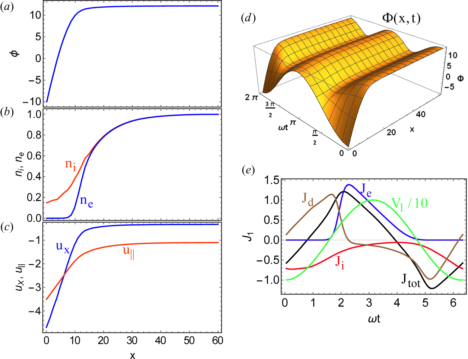
Figure 13. Sample results for an RF sheath with dimensionless parameters ω = 0.5, Ω = 0.25, bx = 0.3, ξ = 10, Jdc = 0 and auxiliary parameters u ||0 = −1.1, μ = 24.17 (deuterium). Panels show the spatial structure of (a) the potential, (b) the ion and electron densities, (c) the ion velocity parallel to b and perpendicular to the plate, all at the time in the RF cycle when the sheath voltage drop is largest, (d) the space–time structure of the potential and (e) the time history of the current waveforms at the plate. All quantities are shown in normalized variables.
Figure 13(d,e) shows some time histories during an RF cycle. Panel (d) illustrates the space–time structure of the electrostatic potential. Note the sinusoidal drive at the wall and the second harmonic at the upstream locations, to be discussed further in § 4.2. The waveforms of the currents at the wall are shown in panel (e). The exponential form of the electron response gives the electron current a very nonlinear (i.e. non-sinusoidal) waveform, which also couples to the other components of the current. In this case all the currents are roughly comparable in size, and each contributes to the total current and to the admittance.
The total DC potential drop across the sheath (i.e. the upstream potential) is 9.19 (Te/e), of which ln μ = 3.19 is from the thermal contribution. The remaining 6.00 (Te/e) is approximately 0.6 of the zero-to-peak potential ξ, a fraction which is typical. The total complex admittance parameter y = 0.0705 − 0.077i. Most of Re(y) is from electrons with Re(ye) = 0.05 and most of Im(y) is from Im(yd) = −0.07. The ions contribute a smaller but not insignificant amount with yi = 0.03 + 0.02i. This distribution of admittance among the components is also typical, with ye gaining in importance at low frequencies, and yd gaining at high frequencies. The ions seem never to dominate and contribute their maximum for ω ~ 1.
4.1.2. Semi-analytical limits
In most cases, numerical methods are required to obtain a solution to the nonlinear fluid equations for the sheath problem. However, in the spirit of providing some concrete examples, a few semi-analytical results are presented next.
One limiting case is the capacitive sheath limit for high-frequency sheaths, already treated heuristically in § 2.2. Here, we recover it from the mathematics. In the high-frequency limit, $\omega \gg {\omega _{pi}}$ , the ion inertia is sufficiently large that the ions are unable to respond on the RF time scale. Mathematically, the ∂/∂t operator in (4.3) and (4.4) is formally large and may be annihilated by time averaging over an RF cycle. This gives conservation of particle flux from (4.3) and conservation of energy from (4.4), where the ion velocity u is determined by the DC field $\langle \varPhi \rangle$
 . Then conservation of flux gives ${n_i} = \langle {n_i}\rangle$
 and the ion response is just as it would be for a biased static sheath with the same DC potential; see (2.6) and containing paragraph. For the perpendicular (i.e. bx = 1) sheath $(u_{x1}^2 - u_{x0}^2)/2 = \langle {\Phi _0}\rangle$
 since $\langle {\varPhi _1}\rangle = 0$
 . In the large RF amplitude limit, ${u_{x1}} = {(2\langle {\Phi _0}\rangle )^{1/2}}$
 and the continuity equation gives the scaling of ni in the sheath as ${n_i}\sim 1/{(2\langle {\varPhi _0}\rangle )^{1/2}}$
 . Even with this simplification, the system is not analytically tractable. However, just as in the static biased sheath, electrons are almost completely excluded from the non-neutral sheath region, and as a result the non-neutral sheath width Δ follows the Child–Langmuir scaling of (2.7) obtained from Poisson's equation by neglecting ne. The admittance is dominated by the displacement current ${J_{dx1}} ={-} {\partial ^2}{\varPhi _1}/\partial x\partial t$
 which is out of phase with ${\varPhi _1} \equiv \xi \cos \varphi$
 , therefore (4.14) recovers the capacitive result ${\hat{y}_{\textrm{sh}}} \approx{-} \textrm{i}\omega /\Delta$
 in agreement with (2.11).
Moving away from the capacitive regime, as the RF frequency decreases, the ions begin to respond to the applied RF voltage, but the temporal variations at frequency ω of ni and u, in the following denoted by ${\tilde{n}_i}$ and $\tilde{\boldsymbol{u}}$
 , are sufficiently small that they may be obtained from a linearization of (4.3) and (4.4). The resulting RF ion current is then given by ${\tilde{\boldsymbol{J}}_i} = {\tilde{n}_i}\bar{\boldsymbol{u}} + {\bar{n}_i}\tilde{\boldsymbol{u}}$
 where the overbar is a shorthand notation for the RF cycle average $\langle \cdots \rangle$
 and for any quantity Q, $Q = \bar{Q} + \tilde{Q}$
 . When the frequency is still high enough that the convective terms may be dropped, i.e. ω > 1, it can be shown that ${\tilde{n}_i}\bar{\boldsymbol{u}} \ll {\bar{n}_i}\tilde{\boldsymbol{u}}$
 and ${\tilde{\boldsymbol{J}}_i} \approx {\bar{n}_i}\tilde{\boldsymbol{u}}$
 (Myra Reference Myra2017) where from (4.4) $\tilde{\boldsymbol{u}}$
 is given by
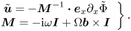
The matrix $\boldsymbol{M}$ is proportional to the familiar cold fluid ion conductivity, and as such has a resonance at the ion cyclotron frequency ω = Ω. After some algebra

and therefore, the ion admittance in this limit is
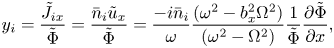
where ${\partial _x}\varPhi /\varPhi \approx{-} 1/\Delta$ and ${\bar{n}_i}$
 , the ion mean ion density in the sheath, should be calculated using a DC sheath model with the appropriate DC bias potential and magnetic presheath density drop. Details are given in Myra (Reference Myra2017). The important point is that this limit provides an analytical result for the ion admittance which, together with other analytical results, are useful in constructing parameterizations and Padè fits for the general case discussed subsequently. In order of magnitude, since ${\bar{n}_i} < 1$
 , (4.17) gives yi < i/(ωΔ) except near cyclotron resonance. Comparing with yd ~ −iω/Δ and noting that the preceding estimates are valid for ω > 1, it follows that except at cyclotron resonance, yi < yd. Numerical results confirm that the ion admittance is usually a relatively small contributor to the total sheath admittance.
As final analytical examples, consider the rectification and electron admittance in the low-frequency limit $\omega \ll 1$ . At low frequencies, the displacement current may be neglected simplifying the application of (4.8) and (4.10). Consider here the case J dc = 0. For the double-plate model, from (4.5)–(4.10), the current conservation condition gives Jx 1 = Jx 2

where φ = ωt. Solving for Φ 0 one obtains
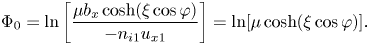
To obtain the final form in (4.19) the low-frequency limit of the ion continuity equation (4.3) has been used to show that ${n_{i1}}{u_{x1}} = {n_{i0}}{u_{x0}} = {u_{x0}} ={-} {b_x}$ in our normalized variables, since the upstream BC on the left half-domain is that ${u_{x0}} = {b_x}{u_{||0}}\;\textrm{and}\;{u_{||0}} \approx{-} 1$
 is directed towards the plate at the sound speed. The rectification effect is then obtained from the RF cycle average

where the ln μ term is the thermal sheath potential, and the remaining integral may be computed numerically as a function of ξ. In the large $\xi \gg 1$ asymptotic limit, it can be shown that $\langle {\varPhi _0}\rangle \sim 2\xi /{\rm \pi} \approx 0.64\xi$
 .
.
The electron admittance ye is obtained similarly in this limit from Je 1 given by (4.8) and the definition of ye in (4.14). Thus, we find
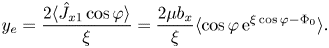
This may be further simplified using (4.19)

which shows that the electron admittance decreases as the magnetic field becomes more tangent to the surface: electrons which are constrained to follow field lines have a reduced projection of current normal to the surface. The electron admittance is also small at high RF voltage because the Maxwell–Boltzmann response is strongly nonlinear, and this results in a small Fourier component at frequency ω. We will return to the topic of nonlinearity in the waveforms.
4.1.3. Parametrizations
A few other analytical results are possible (Myra Reference Myra2017; Myra et al. Reference Myra, Lau, Van Compernolle, Vincena and Wright2020) but in general the sheath rectification and admittance must be computed numerically, as can be done with the NoFlu model over the five-dimensional space indicated in (4.12) and (4.13). In corners of parameter space where asymptotic results are not available, it is usually still possible to ascertain the scaling of the rectification and the individual components of the admittance by heuristic and semi-analytical arguments. Appropriate functional forms with free parameters may then be used as templates for obtaining fits in the various regimes, which can be patched together with Padè-like approximations. The final result of this effort is described in Myra (Reference Myra2017) for the case J dc = 0, and generalized to arbitrary J dc in Myra et al. (Reference Myra, Elias, Curreli and Jenkins2021).
The parametrizations for $\langle {\varPhi _0}\rangle$ and y sh are expressed in terms of analytical functions which have been coded in the Python and Mathematica languages. The fidelity of the parametrizations has been tested against NoFlu computations for many hundreds of representative points spanning the input parameter space. It is found in most cases that the parametrized fits achieve better than 10 % accuracy with respect to NoFlu, and capture correct qualitative trends in all cases checked so far. Further improvements in accuracy are not strongly motivated since the sheath models themselves are unlikely to describe real-world experimental sheaths at a greater level of fidelity than the parametrized fits. The results for y sh are suitable for providing a sheath BC for global RF codes, as described in § 5 and the resulting $\langle {\varPhi _0}\rangle$
 values may be used to model impurity sputtering and other surface interactions.
An illustration of the variation of ${z_{\textrm{sh}}} = 1/{y_{\textrm{sh}}}\propto \hat{z}$ with frequency using the dimensionless parametrized fits is shown in figure 14. Starting from the small $\hat{\omega }$
 (high-density) end of the plot at left, ye is dominant leading to a large $Re (\hat{z})$
 . At $\hat{\omega } = \hat{\varOmega } = 0.1$
 there is a small local increase in Im(z) from the ion cyclotron resonance, but the dominating electrons hide any such feature in $Re (\hat{z})$
 . At $\hat{\omega }\textrm{ = 1}$
 (i.e. the upstream ion plasma frequency) there is a weak broadened resonance, damped because the ions are rapidly leaving the resonance region as they move into the wall. At higher frequencies, the sheath takes on a capacitive character ${\propto}1/\hat{\omega }$
 as the displacement current dominates $\hat{y}$
 and $\hat{z}$
 . The particle contributions, and in particular the electron contribution decreases with increasing $\hat{\omega }$
 (decreasing density).
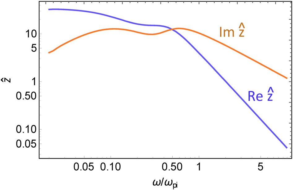
Figure 14. Variation of the dimensionless sheath impedance with dimensionless wave frequency. Other parameters are bx = 0.2, $\hat{\Omega } = 0.1$ , ξ = 10 and Jdc = 0. Some structure is seen at the ion plasma frequency $\hat{\omega } = 1$
 and at the ion cyclotron frequency $\hat{\omega }\textrm{ = }\hat{\varOmega }\textrm{ = 0}\textrm{.1}$
 . Reprinted by permission from figure 2 of Myra & Kohno (Reference Myra and Kohno2019b).
4.1.4. Dimensional (SI) units
In SI units the surface admittance per unit area, i.e. y = the ratio of current density to voltage, is measured in Siemens m−2. Therefore, the dimensionless sheath admittance parameter ${\hat{y}_{\textrm{sh}}}$ is related to the dimensional SI sheath admittance per unit area y sh by
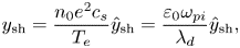
where recall that dimensionless current densities were normalized to n 0ecs and voltages to Te/e. The quantity y sh, or its reciprocal z sh = 1/y sh is what is required for the RF sheath BC discussed in § 5.
4.2. Harmonic generation, nonlinearity and single-ended sheath models
We have already noted that the Maxwell–Boltzmann model for the electrons leads to strongly non-sinusoidal waveforms: if the sheath voltage is assumed to be sinusoidal then the electron current is not; as a result it generates harmonics of the fundamental RF frequency. Nevertheless, it is always possible to project a waveform (the current density waveform in the present formalism) onto the fundamental Fourier component of the applied voltage at the RF frequency. This procedure is appropriate for modelling which only aims to describe the behaviour of the fundamental frequency RF wave where almost all of the power resides. The RF admittance obtained in this way should capture the reflection and absorption properties of the sheath correctly at the fundamental frequency. What is neglected is the possibility that nonlinearly generated harmonics could be launched from the sheath and propagate into the main plasma. Further investigation of the importance of this effect remains as a research topic. As a practical matter, present-day global RF codes are linear in the sense that they only model waves at the fundamental frequency ω. Thus, a more general microscale sheath admittance treatment would find little application at present.
The nonlinear aspects of the microscale sheath model are associated mostly with the electrons and their role in rectification and the electron admittance. It is important to recognize that the results for these quantities in § 4.1 are mildly dependent on the double-plate aspect of the model geometry. A related issue is that the anti-symmetric double-plate model generates harmonics of Φ 0 at even frequencies 2ω, 4ω, 6ω,… as shown in figure 13(d). This happens because Maxwell–Boltzmann electrons respond instantaneously to the electrostatic potential. In particular, as can be seen from the derivation of (4.19), the instantaneous potential at both plates influences the central potential Φ 0 and its time-averaged value. Somewhat different results would be obtained if we were to consider a single-plate system driven by a specified purely sinusoidal RF voltage difference between the upstream location and the plate. In this case in the $\omega \ll 1$ limit, we would have

and the condition that $\langle {J_{x1}}\rangle = 0$ would give
where I 0 is a Bessel function and again for purpose of illustration we assume J dc = 0. This is different from, but qualitatively similar to, (4.20). The asymptotic limit $\xi \gg 1$ in this single-plate system is $\langle {\varPhi _0}\rangle \sim \xi$
 instead of 0.64 ξ. Similar remarks apply to the electron admittance in the single-plate system, which is readily shown to be given by

This is again qualitatively similar to (4.22) for the double-plate model, but different in detail. It is well to keep in mind the model dependence of the electron admittance, a dependence which encompasses both the geometry, the way in which the RF is excited and the validity of the Maxwell–Boltzmann response itself.
The double-plate model is literally applicable for anti-symmetrical near-field antenna sheaths such as might occur for some choices of contact points and antenna strap phasing. It is also applicable in situations which are not obviously driven in an anti-symmetric way, since in the electrostatic model, potentials may be referenced to an arbitrary function of time. Thus, for example, a double-plate model where one plate is grounded, Φ 1 = 0, and the other driven at Φ 2 = −2ξ cos ωt is mathematically equivalent to the anti-symmetrical case Φ 1 = ξ cos ωt and Φ 2 = −ξ cos ωt by shifting the reference ground potential by Φ gnd = ξ cos ωt. This logic, however, assumes that the other conditions of the double-plate model are satisfied, in particular, that the electrons are Maxwell–Boltzmann over the entire domain. If the contact points are far separated, as could occur for magnetically connected far-field sheaths, then collisions may isolate the sheath interactions at the two plates, or (SW) wave propagation may occur along the field lines, both of which are outside the Maxwell–Boltzmann model. In this case, a single-ended sheath description for the electrons, such as in (4.25) or (4.26) may be more appropriate.
The real situation may be even more complicated. In practice, the upstream RF potential drop across the sheath may be neither that of the double-plate model ![]() , or the pure sinusoid plus DC value assumed in the derivation of (4.25) and (4.26). Instead, it may be the result of a self-consistent model of the entire global RF circuit, which could include contributions from cross-field RF currents flowing in the bulk plasma. Nevertheless, the microscale sheath models are not overly dependent on such details. The ion and displacement admittances remain local to a single sheath; the main model differences are to be found in the rectification and electron sheath admittance, which as we have seen, are similar, but not identical, in the double-plate and single-ended models.
, or the pure sinusoid plus DC value assumed in the derivation of (4.25) and (4.26). Instead, it may be the result of a self-consistent model of the entire global RF circuit, which could include contributions from cross-field RF currents flowing in the bulk plasma. Nevertheless, the microscale sheath models are not overly dependent on such details. The ion and displacement admittances remain local to a single sheath; the main model differences are to be found in the rectification and electron sheath admittance, which as we have seen, are similar, but not identical, in the double-plate and single-ended models.
4.3. Kinetic effects
Up until now the discussion of sheaths has been limited to the physics contained in the cold-ion nonlinear fluid model NoFlu. Both static and RF sheaths have been studied with kinetic, primarily, particle-in-cell (PIC) models (Chodura Reference Chodura1982; Perkins Reference Perkins1989; Paes, Sydora & Dawson Reference Paes, Sydora and Dawson1992; Gunn Reference Gunn1997; Ngadjeu et al. Reference Ngadjeu, Faudot, Colas, Heuraux, Gunn and Kubic2011; Jenkins & Smithe Reference Jenkins and Smithe2015; Khaziev & Curreli Reference Khaziev and Curreli2015; Sharma et al. Reference Sharma, Sen, Sirse, Turner and Ellingboe2018). Here, the additional physics provided by kinetic models is briefly summarized.
4.3.1. Kinetic ion physics
Kinetic ion physics brings several new features into the model. The most obvious is the finite Ti increase of the sound speed, ${c_s} \to {c_{si}} = {[({T_e} + {T_i})/{m_i}]^{1/2}}$ which increases the ion saturation current lost to the wall and as a result decreases the (static) thermal sheath potential drop, $\ln [\mu ] \to \ln [\mu /{(1 + {T_i}/{T_e})^{1/2}}]$
 , because the ion flow velocity is a little bit less disparate from the electron thermal speed. In a kinetic model, ions sourced with zero flow and finite Ti do not maintain a constant Ti as they flow to the wall; rather, there is ion acceleration cooling (Stangeby Reference Stangeby2000; Khaziev & Curreli Reference Khaziev and Curreli2015). Nevertheless, it was recently shown (Myra et al. Reference Myra, Elias, Curreli and Jenkins2021) that for eΦrf > Ti the voltage rectification and sheath admittance calculations were practically identical over the range of explored parameters when results from the hPIC (Khaziev & Curreli Reference Khaziev and Curreli2018) and NoFlu codes were compared, if a proper normalization procedure was followed. In particular, the ion saturation currents were specified to be equal in the two cases (requiring a slightly higher density in NoFlu) and that density was used to determine the ion plasma frequency for defining the dimensionless values of ω and Ω. Although the NoFlu model is not singular at the ion cyclotron frequency ω = Ω, (see figure 14 and the discussion of the rapid ion loss from the system) kinetic ion effects were not explored at resonance for the cyclotron frequency or any of its harmonics; ion kinetics may be more important under such conditions. Grazing sheaths for which the magnetic field is nearly tangent to the surface, ${\rm \pi} /2 - \psi = \theta < {(2{\rm \pi} {m_e}/{m_i})^{1/2}}$
 were also not explored in Myra et al. (Reference Myra, Elias, Curreli and Jenkins2021) but some small θ cases are examined in Elias et al. (Reference Elias, Curreli, Jenkins and Myra2021). Additional remarks on grazing sheaths are given in § 6.9.2.
One of the main motivations for carrying out kinetic ion calculations is to determine the ion energy and angle distributions (IEAD) at which the ions strike the surface. The IEAD is of importance for quantifying plasma material interactions. See § 6.8 for a brief discussion.
4.3.2. Kinetic electron physics
The nominal condition for validity of the Maxwell–Boltzmann electron response is

This condition states that the parallel velocity of thermal electrons projected normal to the surface exceeds the velocity of the RF sheath front. Stated another way, the time for a thermal electron to cross the sheath by parallel streaming is shorter than the RF period. The ratios denoted $\textrm{MB} = \omega \Delta /{v_{\textrm{te}}}$ and $\textrm{M}{\textrm{B}_{\textrm{obl}}} = \omega \Delta /{b_x}{v_{\textrm{te}}}$
 are plotted in figure 2(b) for a range of densities in a high-field device with B = 5 T and ω = 2Ωi. It is seen that the Maxwell–Boltzmann condition is satisfied at high densities for field lines that are not too grazing. In Myra et al. (Reference Myra, Elias, Curreli and Jenkins2021), kinetic electron (and ion) PIC results for voltage rectification and sheath currents were compared between the Vorpal (Nieter & Cary Reference Nieter and Cary2004) and NoFlu codes using a similar procedure to that described for hPIC. A case satisfying (4.27) was considered. Kinetic electrons introduce inertia and this was found to trigger ωpe oscillations at the time in the RF cycle when the electron distribution strikes the wall. In these simulations both electron cooling (Stangeby Reference Stangeby2000) and ion cooling occur, complicating the comparisons. After correcting for the different thermal sheath contributions, good agreement in RF voltage rectification was obtained. Current waveforms, suitably normalized and averaged over the fast time scale ωpe oscillations also agreed.
It remains to explore the rectification and admittance differences between Vorpal and NoFlu when (4.27) is marginal or violated. From previous studies (Carter, Batchelor & Jaeger Reference Carter, Batchelor and Jaeger1992; Lieberman & Godyak Reference Lieberman and Godyak1998) it is known that $\omega \Delta \sim {b_x}{v_{\textrm{te}}}$ would give rise to electron heating in a process similar to Fermi acceleration or Landau damping, where the sheath front moves at a velocity that is comparable to that of the electrons. In the extreme limit $\omega \Delta \gg {b_x}{v_{\textrm{te}}}$
 , as could occur in the case where the magnetic field is grazing the surface, a fluid model for the RF part of the electron response is likely to be more appropriate than the Maxwell–Boltzmann model. The grazing case, however, introduces other modelling complications. See § 6.9.2.
4.3.3. Hot electron tails
Although not really kinetic in nature, it is worth mentioning that another generalization of the simple Maxwell–Boltzmann model of (2.4) is that of a two-temperature distribution

where β is the fraction of hot electrons at the upstream location. Hot electron tails abound in laboratory plasmas and are likely present in the SOL of magnetic fusion devices. RF sheaths have been investigated using models of this type (Ou, Xin & Zongzheng Reference Ou, Xin and Zongzheng2019; Myra et al. Reference Myra, Lau, Van Compernolle, Vincena and Wright2020). Not surprisingly, when β is small the tenuous tail population does not have an important effect on electron density, but can change the electron current significantly resulting in modifications to the sheath rectification and admittance. The electron tail population increases the voltage rectification (as required to confine these electrons).
4.4. Other considerations: additional microscale physics; validation
In this tutorial, the intention is to cover only the most basic microscale sheath physics. Additional physics, often included in state-of-the-art static sheath descriptions remains to be studied in the context of high-voltage RF sheaths for fusion devices and its importance in the latter context is, to best of this author's knowledge, unknown. The topic of Fermi acceleration has already been mentioned in passing. Collisions and ionization can be important for sheath physics when the relevant mean free paths are comparable to characteristic scale lengths. On the global scale these effects are frequently important in the presheath, and can have an indirect effect on RF sheaths. The presheath voltage drop itself is usually negligible compared with high power RF sheath voltages. As for the inclusion of collisions and ionization in the sheath itself, in fusion plasmas, the relevant mean free paths are typically far larger than the sheath widths except perhaps for high-voltage sheaths in the divertor region of a detached plasma (low Te, weakly ionized) at near atmospheric neutral pressure or near an antenna where strong neutral gas puffing is employed.
Likely more important, and still needing investigation, are the behaviour of RF sheaths with an ion species mix, and (as a separate topic) RF sheath impedance in the fusion environment taking into account secondary electron emission. Secondary electron emission is discussed briefly in § 6.3, and is treated for static sheaths in e.g. Stangeby (Reference Stangeby2000) and Campanell & Umansky (Reference Campanell and Umansky2017).
Beyond the PIC benchmarking discussed in § 4.3, it would be desirable to have experimental validation of the microscale sheath model, but unfortunately very little is available. Many of the referenced experimental papers are at least consistent with the qualitative predictions expected from an RF-sheath-based theory. However, because of the complexity of the antenna and vessel geometry in fusion experiments, quantitative validation in the fusion setting will likely require complex ICRF simulations that implement the modelling described in this tutorial. In simpler-to-model devices there is a bit more in the way of validation. In unmagnetized plasma in the capacitive sheath regime, Godyak & Sternberg (Reference Godyak and Sternberg1990) report good agreement of sheath rectification calculations with experimental measurements in a mercury vapor discharge. In this regime, the Godyak & Sternberg model is rather similar to NoFlu. Some other aspects of the micro-scale sheath impedance model presented here were validated in experiments on the Large Plasma Device (LAPD), but only within significant limitations (Myra et al. Reference Myra, Lau, Van Compernolle, Vincena and Wright2020). More complete validation awaits modelling implementations in progress.
5. Sheath BC
5.1. Matching condition
As far as waves in the global-scale bulk plasma region are concerned, the effect of the sheath is to present the waves with an effective surface admittance which can absorb them, reflect them (possibly with a phase shift) or partially convert them to other wave polarizations (fast or slow). Expressing the associated BC in terms of the sheath impedance provides the mathematical framework for treating these phenomena.
Since the sheath is normally thin compared with the scale length of variations both along and perpendicular to the surface, a one-dimensional treatment of the BC is almost always appropriate. (Exceptions may occur at special points, such as where the magnetic field is tangent to a point on a sharply curved surface. See § 6.9.2.)
The BC is obtained in the usual way at the interface between two media, by matching the normal component of the displacement vector D or equivalently the normal component of the total current density Jn = n⋅J. The normal component of current on the sheath side of the interface is by construction related to the sheath potential by the sheath admittance. To be more explicit, (4.13) or (4.14) states that the Fourier component at frequency ω of the RF current on the sheath side is related to the RF voltage by Jn ,sh = −y shΦ sh where Φ sh is the RF voltage at the sheath interface relative to the wall and we work in dimensional units. (The sign change is because it is now convenient to regard the wall as grounded and let Φ sh represent the RF plasma potential.) The matching condition Jn ,sh = Jn ,pl, where Jn ,pl is the normal projection of current on the plasma side of the interface, may therefore be stated as $- {y_{\textrm{sh}}}{\Phi _{\textrm{sh}}} = {J_{n,\textrm{pl}}}$ or equivalently as
Taking the tangential gradient, i.e. the components of the gradient along the surface, results in the sheath BC for a sheath on a perfectly conducting surfaceFootnote 8

where it is now understood that Jn is to be evaluated on the plasma side of the sheath interface (since this is a BC to be applied on the plasma side) and ${\boldsymbol{E}_t} ={-} {\nabla _t}{\varPhi _{\textrm{sh}}}$ is continuous across the interface. Equation (5.2) and its companion equation defining ${z_{\textrm{sh}}} = 1/{y_{\textrm{sh}}}$
 in (4.13) and (4.14) are among the most important results of this tutorial paper.
It is worthwhile noting that the parametric dependences of z sh expressed in (4.13) cause it to vary along the sheath surface on the same spatial scale as Jn; therefore, it should be kept inside the gradient, so that the electrostatic condition ${\boldsymbol{E}_t} ={-} {\nabla _t}{\varPhi _{\textrm{sh}}}$ is preserved (as an exact tangential gradient).
Finally, because the physics within the sheath itself is electrostatic it has been natural to present the sheath BC in terms of the scalar sheath impedance parameter z sh. More generally, for electromagnetic wave problems, matching conditions across an interface often employ an impedance matrix connecting the tangential components Et and Bt (Brambilla Reference Brambilla1995). The relationship between these two approaches for the sheath BC is presented at the end of § 6.1.
5.2. Quasi-conducting and quasi-insulating limits
The general sheath BC given in (5.2) has limiting cases which are of practical as well as conceptual interest. The quasi-conducting limit of an RF sheath occurs when the sheath impedance z sh is sufficiently small. The precise meaning of ‘sufficiently’ needs to be deferred to § 6; suffice it to say for now that both Et and Jn relate to wave fields (or near fields) in the plasma, and therefore it can be anticipated that z sh should be compared with a wave impedance. When z sh has a negligibly small value, the sheath BC reduces to Et = 0 which is the usual BC for a perfectly conducting boundary. In this limit, the sheath may be called quasi-conducting. The quasi-conducting limit will typically occur at high density, small RF amplitude and/or low frequency. In the quasi-conducting limit, the sheath voltage z shJn is clearly small: being a good conductor, RF current flow through the sheath results in little RF voltage drop.
The opposite limit is that of the quasi-insulating sheath, for which z sh is sufficiently large. In this case the BC reduces to Jn = 0, equivalent to that of a perfectly insulating boundary. The quasi-insulating limit is mathematically equivalent to the ‘wide sheath limit’ (Colas et al. Reference Colas, Jacquot, Heuraux, Faudot, Crombe, Kyrytsya, Hillairet and Goniche2012) where the case of electrostatic SW polarization is discussed. For the SW polarization, ${J_n} \propto \boldsymbol{n}\boldsymbol{\cdot }\boldsymbol{D = }{\varepsilon _0}\boldsymbol{n}\boldsymbol{\cdot }\boldsymbol{\varepsilon }\boldsymbol{\cdot }\boldsymbol{E} \approx {\varepsilon _0}{b_n}{\varepsilon _{||}}{E_{||}}$ is dominated by parallel physics and the BC Jn = 0 implies E || = 0. Not surprisingly, the quasi-insulating limit tends to give rise to large RF sheath voltages. It typically occurs at low density, large RF amplitude and/or moderate to high frequency.
It would be incorrect to assume that z sh variations cause smooth and monotonically varying sheath effects between the quasi-conducting and quasi-insulating limits. Between these two extremes, there is the possibility that the wave impedance and sheath impedance will form a resonance, analogous to an inductive-capacitive, so-called ‘LC’, resonance in electronics. A discussion of this case, which can produce very large sheath voltages, will also be deferred to § 6. Other non-monotonic variations of z sh were shown in figure 14.
5.3. Poisson-like formulation of the sheath BC
The sheath BC is perhaps expressed in its simplest and most fundamental form by (5.2), namely as a matching condition on the tangential electric field. However, for use in numerical applications, such as discussed in § 6, other implementations are possible.
In one such implementation (Tierens et al. Reference Tierens, Urbanczyk, Colas and Usoltceva2019) the sheath BC is cast into a Poisson-like form using ∇⋅D = 0, i.e.

where ${\nabla _n} = \boldsymbol{n}\boldsymbol{\cdot }\boldsymbol{\nabla }$ is the derivative normal to the surface and Dt is expressed as a linear function of Φ sh given by the solution of some simultaneous equations as follows.
First define the tangential projection operator

Then, applying ${\boldsymbol{P}_t}$ to $\boldsymbol{D} = {\bf \varepsilon }\boldsymbol{\cdot }\boldsymbol{E}$
 yields

If ${\boldsymbol{P}_t}\boldsymbol{\cdot }\boldsymbol{\varepsilon }\boldsymbol{\cdot }\boldsymbol{n}$ were to vanish, the task would be complete since ${{\bf E}_t} ={-} \boldsymbol{\nabla }{\varPhi _{\textrm{sh}}}$
 . However, ${\boldsymbol{P}_t}\boldsymbol{\cdot }\boldsymbol{\varepsilon }\boldsymbol{\cdot }\boldsymbol{n}$
 only vanishes when b and n are parallel or anti-parallel. In general, an additional equation must be employed to express En in terms of Φ sh. That equation is just (5.1) with Jn = −iωDn

or equivalently

Using (5.7) to eliminate En in (5.5) and using Et = −∇tΦ sh we finally have the desired linear relationship between Dt and Φ sh
where
and the last term in (5.9) is to be interpreted as a dyad. Equations (5.3), (5.8) and (5.9) are equivalent to (29) and (30) in Tierens et al. (Reference Tierens, Urbanczyk, Colas and Usoltceva2019) when a capacitive-like form is employed for z sh, i.e. ${z_{\textrm{sh}}} \to \textrm{i}\Delta /(\omega {\varepsilon _{\textrm{sh}}})$ .
.
The Poisson-like character of the formulation, is evident from the quasi-insulating (‘wide sheath’) asymptotic limit where ${z_{\textrm{sh}}} \to \infty$ . In that case (5.3) reduces to
which is just (27) of Tierens et al. (Reference Tierens, Urbanczyk, Colas and Usoltceva2019). That reference also provides a numerical discretization scheme for the Poisson formulation.
5.4. Dielectric layer formulation of the sheath BC
An alternative to the explicit use of a BC that is currently being explored to model sheaths (Beers et al. Reference Beers, Green, Lau, Myra, Rapp, Younkin and Zinkle2021) is to define a thin dielectric layer in such a way that it presents the same surface impedance to the plasma as the sheath BC. In this implementation the layer is made thick enough that it can be resolved by the simulation grid, but still thin compared with other spatial scales in the problem (e.g. geometric scales or wavelengths). The difference in thickness between the dielectric layer and the actual sheath is accounted for in deriving the dielectric properties. A related method was previously explored for the capacitive sheath BC in a plasma processing simulation (Jaeger et al. Reference Jaeger, Berry, Tolliver and Batchelor1995). It can be shown that the dielectric properties of the equivalent layer are given by the complex dielectric constant
where d is the layer thickness. The matching condition across the layer–plasma interface is, as usual, ${\varepsilon _{\textrm{la}}}\boldsymbol{n}\boldsymbol{\cdot }{\boldsymbol{E}_{\textrm{la}}} = \boldsymbol{n}\boldsymbol{\cdot }{\boldsymbol{\varepsilon }_{\textrm{pl}}}\boldsymbol{\cdot }{\boldsymbol{E}_{\textrm{pl}}}$ , where Ela is the electric field in the layer. The sheath voltage is then given as ${\varPhi _{\textrm{sh}}} ={-} d\boldsymbol{n}\boldsymbol{\cdot }{\boldsymbol{E}_{\textrm{la}}}$
 or explicitly

independent of the layer thickness and in agreement with (5.1).
5.5. Dynamic sheath BC in the time domain
The formulations of the sheath BC discussed in the preceding §§ 5.1, 5.3 and 5.4 apply to frequency-domain codes which, having Fourier transformed in time, allow algebraic dependence on the RF frequency ω. Time-domain electromagnetic codes have also been used for sophisticated RF modelling (Smithe Reference Smithe2007) including highly detailed three-dimensional geometry, and the nonlinear evolution of the sheath potential (Smithe, D'Ippolito & Myra Reference Smithe, D'Ippolito and Myra2014; Jenkins & Smithe Reference Jenkins and Smithe2015). In this time-domain approach, the effective sheath capacitance and resistance are included in lumped circuit model equations that are evolved on the bounding surfaces. The parameters of the lumped circuit elements can be tuned to match the impedance from the microscale model. The procedure has been successfully benchmarked against first principles PIC simulations in the capacitive sheath regime (Jenkins & Smithe Reference Jenkins and Smithe2015).
In the time domain, the DC sheath potential may be obtained directly from the amplitude envelope of the RF sheath voltage, for example by implementing a lumped circuit rectification and low-pass filter model. The amplitude information may then be used to tune the nonlinear dependence of the capacitance (through the sheath width Δ) and resistance in the lumped circuit model directly in the time evolution, obviating the need for the nonlinear iteration that is necessary in frequency-domain codes (§ 5.7).
This is a significant advantage of the time-domain approach that may be especially important when the nonlinearity of the RF sheath BC gives rise to multiple roots, as discussed in § 6.2. It is expected that a time-domain simulation should automatically select the physical root. Time-domain codes have not yet, to the author's knowledge, been applied in multiple root cases, but this should be a fruitful area of application.
5.6. Sheath post-processing
Although implementation of the sheath BC in full wave RF codes is required for accurate modelling, it is possible under some limitations to gain information about RF sheaths from codes which implement the more conventional perfectly conducting wall (CW) BC, Et = 0 using a sheath post-processing method (Myra & Kohno Reference Myra and Kohno2019a). The basic idea relies on the assumption that, observing from the surface, the incoming waves are not affected by whether the BC is the CW BC or the sheath BC. (An exception would be a resonant cavity or other situation where multiple reflections are important.) If the incoming waves are fixed, it is possible, given sufficient information at the surface under one type of BC, to transform the outgoing waves (and hence the total electric field) to another solution under a different type of BC using calculations purely local to the surface.
This procedure was demonstrated using semi-analytical methods, to yield exact sheath BC results for flat walls and constant plasma parameters on the surface; and approximate results for curved walls using local theory. The input required from the CW solution is Jn on the surface, and the output is Φ sh. The post-processing method is not expected to be useful for sheaths in complicated three-dimensional geometries.
5.7. Nonlinear iteration of the sheath BC
When frequency-domain methods are used to implement the sheath BC, some form of iteration is required to handle the nonlinearity that arises from the dependence of z sh on the wave amplitude, as expressed through ξ in § 4.1. This nonlinearity is related to, but conceptually different from, the nonlinear waveforms that appear internally in the microscale modelling (See figure 13e). Here, we are concerned only with the effect of the RF amplitude; the nonlinear time dependence has already been projected onto the Fourier mode ω of interest.
To illustrate this conceptually we consider here a simple fixed-point iteration scheme. More sophisticated iteration or root-finding schemes such as the Newton–Raphson method (Kohno & Myra Reference Kohno and Myra2017) may, however, prove useful. A fixed-point algorithm would proceed as follows:
(i) Make an initial guess for z sh (e.g. the CW limit z sh = 0).
(ii) Solve the global RF problem with the sheath BC using the current value of z sh.
(iii) From the solution, obtain Jn at each point on the boundary; calculate ${\varPhi _{\textrm{sh}}} ={-} {z_{\textrm{sh}}}{J_n}$
 and then $\xi = |e{\varPhi _{\textrm{sh}}}/{T_e}|$.
(iv) Update z sh = 1/y sh at each boundary point with the new value of ξ using a microscale model or its parametrization ${\hat{y}_{\textrm{sh}}}(\hat{\omega },\hat{\Omega },{b_x},\xi ,{\hat{J}_{\textrm{dc}}})$
.(v) Go to step (ii) until convergence is achieved.


Fixed-point iteration has been implemented in several codes including a COMSOL workflow (Beers et al. Reference Beers, Green, Lau, Myra, Rapp, Younkin and Zinkle2021), codes under development in the US RF SciDAC project (Bonoli et al. Reference Bonoli and Green2020) and SSWICH in the EU (Tierens et al. Reference Tierens, Urbanczyk, Colas and Usoltceva2019). It has been shown to converge rapidly (fewer than a dozen iterations) in one-, two- (Myra & Kohno Reference Myra and Kohno2019a) and three-dimensional (Beers et al. Reference Beers, Green, Lau, Myra, Rapp, Younkin and Zinkle2021) cases where the boundary shapes were relatively simple and parameters where not close to multiple root conditions (§ 6.2). Convergence properties for a realistic three-dimensional antenna tokamak geometry remain to be investigated.
In cases where the sheath is ultimately expected to be in the quasi-insulating limit, it may be logical to begin the iteration with the guess z sh = ∞, i.e. perfectly insulating BCs. In this case step (iii) on the first iteration must be modified since Jn will be zero. A suitable procedure would be to solve (5.10) or simply use it to estimate a reasonable order of magnitude guess for Φ sh on the first loop of the iteration. Alternatively, one could choose z sh in step (i) to be finite but sufficiently large (${\hat{z}_{\rm sh}}\, > > 1$ ) so that Φ sh = −z shJn in step (iii) is still a numerically well posed calculation.
6. Macroscale RF sheath effects
Up until now, except for § 3, this paper has been mostly focused on the microscale description of the RF sheath. The goal of the present section is to describe some of the global (macroscale) effects of RF sheaths on the plasma and in particular on the RF waves that propagate in the plasma volume.
6.1. Sheath and wave impedance
Section 5 characterizes the sheath impedance and introduces its two limiting cases, the quasi-conducting and quasi-insulating limits. We are now in a position to discuss the conditions under which the RF sheath behaves in these limits, because these conditions depend on the impedance of the RF waves that are interacting with the sheath.
The basic concepts and sheath interaction regimes were calculated in a semi-analytical one-dimensional model for the electrostatic SW in Myra & Kohno (Reference Myra and Kohno2019b). Consider a plane wave incident on a flat surface on which there is an RF sheath. The geometry is illustrated in figure 15. The background magnetic field is at an arbitrary angle to the surface. In general, the wave-sheath interaction will result in a reflected wave with complex reflection coefficient Ar, and possibly some amount of RF power absorption by the sheath. In a uniform plasma, the total electrostatic potential may be represented as

Here, k1 and k2 are the two (incoming and outgoing) wavevectors that solve the electrostatic SW dispersion relation

where $\boldsymbol{\varepsilon }$ , ε ⊥ and ε || are given in the text following (3.2) and the notations ⊥ and || refer to perpendicular and parallel with respect to the background magnetic field. In the one-dimensional problem the components of k tangential to the surface are regarded as given, and the normal component is obtained from the dispersion relation. Note that k 2n = −k 1n only if b and n are parallel (or anti-parallel) so that k⊥ = kt and k || = kn. (Remember that n is the unit surface normal, not the index of refraction vector. Since the present section is electrostatic, no confusion should result.)

Figure 15. Geometry of a plane wave interaction with a sheath. Reprinted by permission from figure 1 of Myra & Kohno (Reference Myra and Kohno2019b).
It is a straightforward exercise to compute E = −∇Φ from (6.1), ${J_n} ={-} \textrm{i}\omega {\varepsilon _0}\boldsymbol{n}\boldsymbol{\cdot }\boldsymbol{\varepsilon }\boldsymbol{\cdot }\boldsymbol{E}$ and then apply the sheath BC ${\boldsymbol{E}_t} = {\nabla _t}({z_{\textrm{sh}}}{J_n})$
 to solve for the reflection coefficient Ar. Noting that ${\boldsymbol{k}_{t1}} = {\boldsymbol{k}_{t2}} \equiv {\boldsymbol{k}_t}$
 since kt is specified, and carrying out the algebra results in Myra & Kohno (Reference Myra and Kohno2019b)

where
The preceding equation implicitly defines the wave impedance zwj and its reciprocal, ywj = 1/zwj the normal wave admittance for a plane electrostatic wave with wave-vector k, i.e.
where bn = b⋅n.
It is now clear that the quasi-conducting limit applies when $|{\rho _j}|\ll 1(\kern0.06em j = 1,2)$ . In this case Ar = −1 and the sheath reflects the wave as if it were a perfectly CW. Conversely, for $|{\rho _j}|\gg 1$
 the result is ${A_r} ={-} {\rho _1}/{\rho _2}$
 . If, in addition to being large, ${\rho _1} ={-} {\rho _2}$
 as it does when b and n are parallel (or anti-parallel), the sheath BC is in the quasi-insulating limit, Ar = 1 and the sheath reflects the wave just as if it were a perfect insulator. In general, the ρj are complex numbers and it can be shown (Myra & Kohno Reference Myra and Kohno2019b) that for propagating waves (i.e. kj pure real), the fraction of incident power per unit area that is absorbed by the sheath is
and that the power per unit area absorbed by the sheath is ${P_{rf}}/A = {f_P}|{\varPhi _{rf}}{|^2}Re({y_{w1}})/2$ . Additional discussion of power dissipation in the sheath and power balance is given in § 6.3 where the power dissipation is given in terms of y sh and $|{\varPhi _{\textrm{sh}}}{|^2} = |1 + {A_r}{|^2}|{\varPhi _{rf}}{|^2}$
 .
.
For ρ 1 = 1, which gives Ar = 0, one has impedance matching and the waves are completely absorbed by the sheath.Footnote 9 Finally, for ρ 2 = 1 we encounter a resonance, formally Ar = ∞. This special case is known as the sheath–plasma resonance, and is the topic of the next subsection.
The preceding discussion is specialized to electrostatic SWs. It can be generalized to the electromagnetic case by introducing a sheath impedance matrix Z defined by
where the definition is motivated by Brambilla (Reference Brambilla1995) and Senior & Volakis (Reference Senior and Volakis1991). Substituting $\boldsymbol{J} = \textrm{i}\boldsymbol{k} \times \boldsymbol{B}/{\mu _0}$ , (where as elsewhere J contains both particle and displacement currents) into the sheath BC ${\boldsymbol{E}_t} = \textrm{i}{k_t}{J_n}{z_{\textrm{sh}}}$
 yields the sheath impedance matrix for plane waves,
The interaction of waves at the sheath surface then involves the product ${\boldsymbol{Z}_{\rm sh}}\boldsymbol{\cdot }{\boldsymbol{Y}_j}$ where ${\boldsymbol{Y}_j}$
 is the wave admittance matrix of the FW or SW in question.
The coupling of FWs and SWs by the sheath BC is discussed in § 6.4. Here, we note that the electrostatic parameter ρj is replaced by a vector triple product, (6.28), involving a combination ${k_t}\omega {\varepsilon _0}{z_{\textrm{sh}}}(\boldsymbol{n}\boldsymbol{\cdot }\boldsymbol{\varepsilon }\boldsymbol{\cdot }{\boldsymbol{e}_j})$ which is rather similar to ρj, where ej is the unit polarization vector for the fast or SW.
6.2. Sheath–plasma resonance
The condition ρ 2 = 1 specifies that z sh = zw 2, i.e. the outgoing wave impedance matches the sheath impedance. An intuitive understanding of the sheath–plasma resonance is most straightforward in the perpendicular sheath limit |b⋅n| = 1, which will be considered for the rest of this discussion. In that case zw 2 = −zw 1 and the condition is

This is just the condition for a series resonance of two circuit elements, the so called ‘tank circuit’ that exists between a capacitor with positive imaginary impedance and an inductor with negative imaginary impedance.
The simplest sheath–plasma wave interaction example is that of a capacitive sheath, ${z_{\textrm{sh}}} = \textrm{i}\Delta /(\omega {\varepsilon _0})$ from (2.11), interacting with an electron plasma wave (SW). The SW admittance from (6.5) is, retaining only the dominant ε || term,

For an inductive-like response, the SW must be evanescent, i.e. k ||,1 pure imaginary. Considering the electrostatic dispersion relation, (6.2), this can happen for real k ⊥ at sufficiently high density such that ε ⊥ < 0 and ε || < 0. In the geometry of figure 7(a) or figure 12 with b = n = ex, and considering the left sheath, the incoming wave, exp(ik1⋅x), must decay towards the wall, which requires k ||,1 = −iκ with $\kappa = {(k_ \bot ^2{\varepsilon _ \bot }/{\varepsilon _{||}})^{1/2}} > 0$ . This gives the inductive-like response
Physically, the response arises from the parallel electron current reacting against the parallel electric field. The sheath plasma resonance condition (6.7) in this specific case, reduces to

The outgoing wave is amplified by the resonance (an infinite amount in this idealized example) and has ${k_{||,2}} ={+} \textrm{i}\kappa$ . It decays away from the surface and dominates the total wave field. Not only must (6.12) be satisfied but also the dispersion relation, (6.2), which requires a finite k ⊥ (tangential to the surface in this example). This solution is therefore also referred to as a sheath–plasma wave propagating along the surface.
Sheath–plasma waves (resonances) have been known for many decades (Bekefi Reference Bekefi1966; Stenzel Reference Stenzel1988) and studied in RF plasma discharge cells (Lieberman et al. Reference Lieberman, Lichtenberg, Kawamura, Mussenbrock and Brinkmann2008). More recently, they have been observed in global RF simulations employing a sheath BC (D'Ippolito et al. Reference D'Ippolito, Myra, Jaeger and Berry2008; Kohno & Myra Reference Kohno and Myra2017). In (Kohno & Myra Reference Kohno and Myra2017) global RF simulations demonstrate some cases in which the generalized sheath BC, i.e. retaining ion and electron contributions to the sheath impedance, resolve the resonant singularity and in some cases completely destroy the sheath–plasma resonance. Whether the resonance occurs in practice will depend in part upon the relative importance of dissipative to capacitive contributions in z sh.
Finally, note that the sheath width Δ appearing in (6.12) depends on the RF wave amplitude through the Child–Langmuir relation (2.7) in the capacitive model; more generally, z sh in (6.9) depends on ξ as expressed in (4.13). This means that the resonance may occur for particular values of Φ rf, multiple roots can occur (D'Ippolito et al. Reference D'Ippolito, Myra, Jaeger and Berry2008; Kohno, Myra & D'Ippolito Reference Kohno, Myra and D'Ippolito2012) and there can be positive feedback between the amplification of Φrf and the approach to resonant conditions. In a driven problem (e.g. by antenna or fixed wave impinging on the sheath) the self-consistent solution for Φ rf plotted against a parameter such as density or magnetic field inclination usually exhibits a familiar ‘S-shaped’ curve. See for example figure 6 of D'Ippolito et al. (Reference D'Ippolito, Myra, Jaeger and Berry2008). Thus, there can be 1 or 3 roots (2 at the special case of inflection points).
When several roots are possible mathematically, the procedure for deciding which root is physical is not obvious. At very low RF voltages, only 1 root exists (at least in the cases examined in the literature). As the RF voltage is increased and multiple roots appear, it is usually assumed that the physical root is the one that tracks continuously from the single root condition. At some point it may happen that continuous root tracking is no longer possible and then the root must jump from the low-voltage root to the high-voltage root. The middle ‘S-shaped’ root is usually assumed to be an unstable fixed point. Demanding continuity of roots, when possible, in general leads to hysteresis if the multiple root regime is approached from the high-voltage side. It remains to investigate multiple root cases in realistic three-dimensional geometry. A time-domain approach (§ 5.5) may provide the best answer to root selection in these cases.
A different example of the effect of wave amplitude on the structure of the sheath–plasma wave solution is shown in figure 16 from (Kohno & Myra Reference Kohno and Myra2019). In this case the small amplitude solution at left, figure 16(a), is far from sheath–plasma resonance and the wave-field pattern remains linear, with a sheath BC that is almost that of the thermal sheath. The large amplitude solution at right, figure 16(b) is close to sheath–plasma resonance. Parameters other than the wave amplitude are the same in the two cases. The spreading of the waves in the y-direction is the damped propagation of the sheath–plasma wave. Both solutions solve the self-consistent problem (i.e. with iteration) using the generalized sheath BC. Note that the colour palette has been scaled with the antenna current to enable better comparison of the wave-field structures.

Figure 16. RF wave field Re (E ||) contrasting two cases: (a) a linear case with very small antenna current of 1 A m−1 and (b) a nonlinear case near sheath–plasma resonance with antenna current 100 A m−1. Both solutions solve the self-consistent problem (i.e. with iteration) using the generalized sheath BC. The thick black line at x = 0.47 m is a model antenna and the sheath is located on the wall at x = 0.50 m. Reprinted by permission from figure 4 of Kohno & Myra (Reference Kohno and Myra2019).
6.3. Sheath power dissipation, surface heat load and power balance
The amount of RF power dissipated in the sheath, the heat load on the material wall surface from particle impact and an understanding of power transfer and overall energy balance in the RF sheath are of great importance. These topics are more subtle than might appear at first glance.
The power dissipation per unit volume within the sheath is given as usual by J⋅E. In general, this can be divided into contributions from the DC and RF parts of J and E. Considering the RF contribution for waves varying in time as exp(−iωt), the net power dissipated per unit volume is

Integrating over the volume of the sheath, again regarding x as the variable normal to the surface one obtains the net power dissipation per unit sheath area A as

This expresses the sheath power dissipation in terms of the RF sheath potential Φ sh. See also (6.6) and the following text which expresses the sheath power dissipation in terms of the incident wave amplitude Φ rf. The equivalence of these two expressions is proved in appendix B of Myra & Kohno (Reference Myra and Kohno2019b). Here, ∞ in the integration is to be interpreted as the sheath edge (sheath entrance) and the fact has been used that the total Jn (including displacement as well as particle currents) in the sheath is spatially constant (see the discussion immediately following (4.7)) and matched to the plasma side of the sheath. The final step invokes the definition of ${y_{\textrm{sh}}} \equiv 1/{z_{\textrm{sh}}}$ in (5.1). Thus, once a self-consistent solution for the potential drop across the sheath, Φ sh (= Φ 0–Φ 1 in the notation of the microscale model) has been found, the RF part of the sheath dissipation is readily computed. It will be shown below that this power appears as a heat load on the surface. It also contributes to RF edge losses that are often observed in experimental scenarios, especially when single pass absorption is low, or significant wave fields exist in the boundary region, e.g. due to coaxial modes (Messiaen & Maquet Reference Messiaen and Maquet2020). A caveat is that, in accord with remarks made in § 4.2, the treatment of y sh given here relates only to the fundamental RF frequency at ω, ignoring harmonics. A more general expression for power dissipation taking into account all harmonics should really be employed in cases where the electron current is strongly nonlinear.
Similar remarks apply to the DC parts of J and E in the case where the sheath carries net DC current. The sheath behaves as a resistor that converts the electrical energy into heat

where here and in (6.14) Jn is negative when there is net ion current flowing into the left sheath of figure 12.
For some plasma–material interactions such as surface melting, a quantity of interest is the net power per unit area incident on the surface. Expressing the result from (Stangeby Reference Stangeby2000) in the present notation we have the dimensionless heat flux at the wall x = x 1 given as

Here, ${n_{i1}}{u_{x1}} < 0$ is the x-component of the ion particle flux at the wall, 2.5 Ti is the thermal heat flux where 2.5 is an approximate model-dependent coefficient (Stangeby Reference Stangeby2000), ${\varPhi _{\textrm{sh}}} = {\varPhi _0}\; - {\varPhi _1} > 0$
 is the (total RF + DC) potential drop that the ions fall through, and the last term is the electron thermal energy, i.e. 2Te times the electron particle flux at the wall.
It is important to distinguish between the heat flux at the wall and the heat flux at the sheath entrance, x = x 0 (‘upstream’ in our nomenclature, but not far enough upstream to include the source presheath). At the sheath entrance we have

Here, in dimensionless units ${n_{i0}} = 1,\;{u_{x0}} ={-} {b_x}$ and we have allowed for secondary electron emission with coefficient δ se in the electron term. Note that the magnitude of the electron particle flux is reduced by the secondary electron emission

but the heat flux from incident electrons at the wall does not depend on δe (Stangeby Reference Stangeby2000). At this upstream location, the ions have not yet been accelerated through the sheath but the electrons have additional kinetic energy since they have not yet been slowed down by the potential.
With the caveat that the 2.5 Ti coefficient has not been readdressed for the RF case, (e.g. ion jitter motion in the RF fields has not been accounted for, but is expected to be small), we can apply these expressions to obtain an understanding of the mean surface heat load in the RF case, and the role of the sheath and the RF waves on power balance.
The time averaged fluxes expressed in terms of the dimensionless signed current are

at the wall, and

at the sheath entrance. Here, $\langle {J_{xi0}}\rangle = \langle {J_{xi1}}\rangle$ from the ion continuity equation, $\langle {J_{xe0}}\rangle = \langle {J_{xe1}}\rangle$
 and the DC current flowing through the sheath is

Combining equations (6.19) and (6.20) results in

Neglecting the second harmonic contribution to power balance (see § 4.2) we take ${\varPhi _{\rm sh}} = \langle {\varPhi _{\rm sh}}\rangle + {\tilde{\varPhi }_{\rm sh}}$ where ${\tilde{\varPhi }_{\rm sh}}$
 is the RF driving voltage. Then using (6.21)

or equivalently,

This demonstrates that the DC and RF electrical power dissipated in the sheath adds to the incoming heat flux at the sheath entrance, and ultimately appears on the wall surface.
In Myra & Kohno (Reference Myra and Kohno2019b) it was shown, albeit for the special case of SWs, that the power lost in the RF wave energy flux is equal to the power dissipated in the sheath when the sheath BC is employed. Thus, we can assert that the RF waves ultimately supply the power that is needed to maintain the RF-enhanced sheath-rectified potential and that this power appears at the plate in the form of enhanced ion heat flux.
This sub-section is closed with a brief remark about the effect of secondary electron emission on RF sheaths. Because μ is large, i.e. the electron thermal velocity is large compared with the sound speed, the electron fluxes at the wall also tend to be large. The sheath self-biasing including RF sheath rectification reduces the large electron flux, but at the price of creating high energy ions which enhance sputtering. As the secondary electron coefficient δ se increases, the electron current is reduced and with it the rectified RF potential, and the sputtering. The same reduction in Φ 0 also occurs if we simply allow the surface to draw a large electron current (Stangeby Reference Stangeby2000; Perkins et al. Reference Perkins, Hosea, Jaworski, Bell, Bertelli, Kramer, Roquemore, Taylor and Wilson2017). Under these circumstances the total heat flux (which, being specified upstream, is a given as far as the RF sheath is concerned) is transferred from the ion channel to the electron channel. Although this does not affect the total power deposition on the surface, it may be beneficial for reducing sputtered impurities.
6.4. FW to SW conversion
As introduced heuristically in §§ 3.3 and 3.4, although the SW polarization is directly responsible for strong RF sheath interactions, FWs incident on the surface can also generate RF sheaths because of boundary-induced mode conversion between the FW and SW polarizations. In the present section, this is investigated in more detail.
The basic mechanism of the interaction can be understood in a slab geometry with plane waves (D'Ippolito et al. Reference D'Ippolito, Myra, Jaeger and Berry2008). The surface is the plane x = 0. The total electric field may be represented as
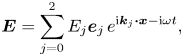
where E 0e0 is the incident FW, E 1e1 is the reflected FW, and E 2e2 is the reflected SW. Here, ej is the unit polarization vector of each mode (not to be confused with the Cartesian coordinate directions), ω is assumed to be given along with ky and kz (i.e. the components of kt tangent to the surface) and the normal component kx is determined from the dispersion relation. The polarization vectors ej may be determined analytically when the fast and slow branches are well separated (D'Ippolito et al. Reference D'Ippolito, Myra, Jaeger and Berry2008), but the formalism remains valid in the case of mode confluence. It should be noted that in general, ${k_{x1}} \ne - {k_{x0}}$ for an oblique magnetic field, and ${\boldsymbol{e}_0}\; \ne {\boldsymbol{e}_1}$
 because the polarization vectors depend on kx.
Applying the sheath BC, (5.2) using ${J_n} ={-} \textrm{i}\omega \boldsymbol{n}\boldsymbol{\cdot }\boldsymbol{\varepsilon }\boldsymbol{\cdot }\boldsymbol{E}$ and crossing with n to extract the tangential components results in the condition at the sheath surface (x = 0)
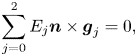
where
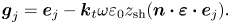
(Recall that n is the surface normal, not the index of refraction. The latter quantity will not be employed in this section.) Dotting (6.26) with g1 or g2 allows the amplitudes of the reflected (propagating or evanescent) branches, E 2 and E 1 respectively, to be determined. For the SW branch, one obtains
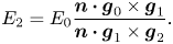
From the previous equation it is clear that there are conditions which make the denominator small (resonance) and other conditions which make the numerator small. In the case where the SW is electrostatic, e2 ∝ k, one recovers the electrostatic sheath–plasma resonance condition where the magnitude of g 2t vanishes. This is just the condition ρ 2 = 1 of (6.3) and (6.4) In the electromagnetic case here, it is possible for the cross product in the denominator to become small by virtue of the directions of gj.
The numerator involves the FW quantities g0 and g1. For modest values of kt the second term in (6.27) is often not large for FWs because ej has a negligible parallel component. This eliminates the large term ε || and, assuming the terms involving ε ⊥ and ε × are small, the numerator of (6.28) reduces to n⋅e0 × e1. One can immediately see that in the case of a normal incidence magnetic field, i.e. bn = 1, there can be no SW generated because e0 = e1. (The FW polarization is independent of the sign of k ||.) RF wave interactions with the wall require oblique incidence if a SW and significant RF sheath are to be generated. In practical terms it means that far-field FW sheaths in a tokamak occur on material surfaces that do not conform to magnetic flux surfaces. Other properties are discussed in D'Ippolito et al. (Reference D'Ippolito, Myra, Jaeger and Berry2008).
In this model we can expect the largest RF sheath voltages driven by incident FWs to occur for conditions of oblique incidence and parameters close to sheath plasma resonance. The latter condition typically requires kt to be ‘large’ i.e. large enough to satisfy ${g_{2t}} \ll 1$ . Although it is outside the scope of our simple slab model, we can argue heuristically that a FW incident on a sharply curved surface necessarily acquires an effective kt at the surface that is large. For this reason, FW to SW conversion is expected to be prominent near places where the local magnetic field incidence angle parameter bn changes rapidly along the surface. Referring back to figure 10, in particular 10(c), this is indeed seen to be the case in a far-field simulation which incorporated a curved wall impacted by an incident FW (Kohno, Myra & D'Ippolito Reference Kohno, Myra and D'Ippolito2015).
6.5. RF-driven convection
From § 4 we know that RF sheaths are associated with rectification, i.e. the formation of large DC potentials on field lines in the global plasma. The size of the potential on a particular field line depends primarily on the amplitude of the RF waves where the field line contacts the surface, and as well on other parameters as described in (4.12). Because adjacent field lines can contact different surfaces on a complicated three-dimensional structure like an antenna, and because RF amplitudes can vary rapidly along some surfaces, these adjacent field lines charge up to different electrostatic potentials. The good parallel electrical conductivity of the plasma relative to its perpendicular conductivity enforces DC electric fields which are weak in the parallel direction but can be strong in the perpendicular direction. The result is that RF dominated edge plasmas are often subject to strong E × B drifts. This convection can impact the density profile near an antenna, thus affecting the antenna coupling and the particle and heat fluxes on nearby surfaces and the resulting impurity generation.
A low particle confinement H-mode was triggered on the JET experiment during ICRF operation in monopole phasing, a phasing which should generate the strongest RF sheaths and convection. (See figure 9(a) and its discussion for an explanation of the role of phasing.) The H-mode interaction and increased particle transport across the separatrix was attributed to the formation of separatrix-crossing convective cells as illustrated in figure 17 (D'Ippolito et al. Reference D'Ippolito, Myra, Jacquinot and Bures1993). In experiments from the same era, large-scale convection was observed surrounding the antenna on the Tore Supra tokamak (Bécoulet et al. Reference Bécoulet, Colas, Pécoul, Gunn, Ghendrih, Bécoulet and Heuraux2002). Additional experimental evidence is summarized in Colas et al. (Reference Colas, Ekedahl, Goniche, Gunn, Nold, Corre, Bobkov, Dux, Braun, Noterdaeme, Mayoral, Kirov, Mailloux, Heuraux, Faudot and Ongena2007). More recently, Zhang et al. (Reference Zhang, Tierens, Noterdaeme, Bobkov, Aguiam, Coster, Fuenfgelder, Jacquot, Ochoukov, Silva, Colas and Křivská2017) has modelled ICRF-driven convection near an antenna in ASDEX Upgrade and Hong et al. (Reference Hong, Wukitch, Lin, Terry, Cziegler, Reinke and Tynan2017) has employed gas puff imaging to measure ICRF-driven convection velocities on Alcator C-Mod and thereby infer the rectified potential amplitudes. RF-driven convection in lower-hybrid (LH) experiments was also observed in Alcator C-Mod especially on field lines that were magnetically connected to the LH launcher (Lau et al. Reference Lau, Hanson, Labombard, Lin, Meneghini, Ochoukov, Parker, Shiraiwa, Terry, Wallace, Wilgen and Wukitch2013). ICRF-driven convective cells were also observed in the linear LAPD device (Martin et al. Reference Martin, Gekelman, Van Compernolle, Pribyl and Carter2017).
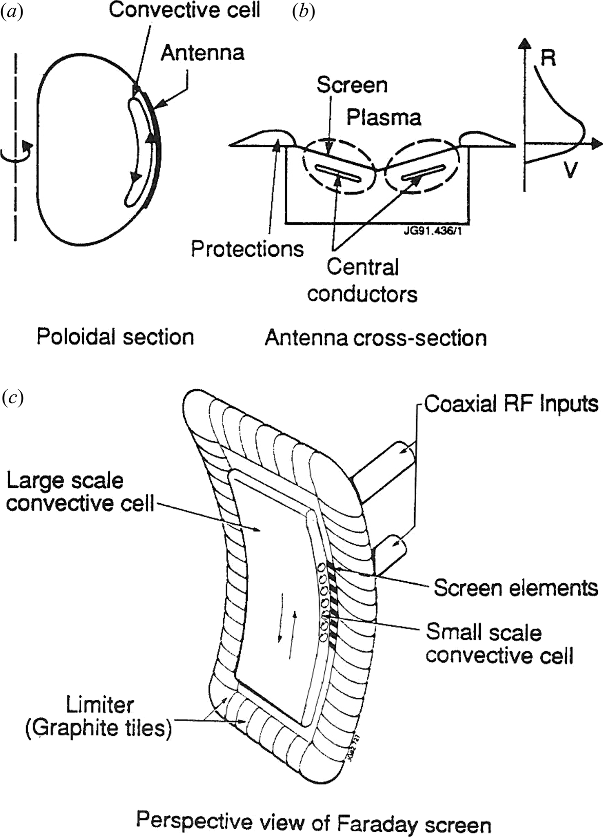
Figure 17. Illustration of some different types of convective cells that can form around an antenna. Reprinted by permission from figure 3 of D'Ippolito et al. (Reference D'Ippolito, Myra, Jacquinot and Bures1993).
An interesting aspect of RF-driven convection is its interaction with plasma turbulence. In the SOL, such turbulence is manifest in the formation of blob filaments (Krasheninnikov, D'Ippolito & Myra Reference Krasheninnikov, D'Ippolito and Myra2008). Not surprisingly, the strongly sheared flows from RF-driven convection can shear and even tear apart the blobs as shown in theoretical studies (Myra et al. Reference Myra, D'Ippolito, Russell, Berry, Jaeger and Carter2006) and observed in experiments (Zhang et al. Reference Perkins, Hosea, Taylor, Bertelli, Kramer, Luo, Qin, Wang, Xu and Zhang2019). Sheared flows could also drive turbulence, as discussed briefly in § 6.7.
6.6. Global DC circuits
In a real tokamak, sheaths exist on a variety of different surfaces with different plasma and magnetic field parameters and driven by different RF field amplitudes. A highly schematic illustration of this type of situation is shown in figure 18. On a given field line or flux tube, the sheaths at the two different ends are usually not symmetric, except perhaps in the special case of certain near-field antenna sheaths. From § 4, it will be recalled that the rectified (DC) voltage in the plasma, i.e. at the sheath entrance, will therefore be different at the points A, B, D and E in figure 18. In general, this will drive currents flowing both through the plasma and in the vessel walls. The DC current–voltage relationship, represented as a resistance in the figure, will determine the currents in the various paths. In the plasma, the current can flow both along and across field lines. Of course, the parallel conductivity in a plasma is many orders of magnitude larger than the perpendicular conductivity, but on sufficiently long field lines the net perpendicular current flow may be competitive.
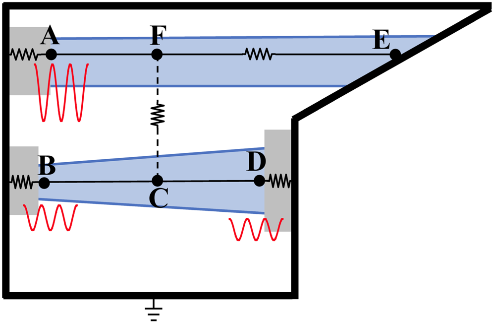
Figure 18. A conceptual illustration of asymmetrical RF sheaths and the associated DC current paths in a complex structure. The thick black line represents a grounded wall. Magnetic field lines (solid black) and associated flux tubes (blue) provide current paths with volume resistance illustrated between E and F and terminated by effective DC sheath resistances at A, B and D. A cross-field current path (dashed black) and associated resistance is illustrated between C and F. The RF amplitude driving the sheaths (grey and shown with a greatly exaggerated scale) is large at A, smaller and B and D and negligible at E. The expanding flux tube between B and D indicates a different magnetic field strength at those locations, and the magnetic field angle is different at E than at A.
Whole device modelling of this in a real tokamak would be a daunting task. The DC current–voltage relationship for the sheath is not only nonlinear, but nonlinearly coupled to the RF wave amplitudes at the surface, which in turn must be determined from global full wave solvers using the sheath BC. Furthermore, the DC sheath potential and RF sheath impedance in that BC are dependent on the DC currents flowing through each patch of sheath.
As if that were not enough, the cross-field conductivity in a fusion SOL plasma is expected to be determined by turbulence rather than classical collisional processes. This could, in some cases, be the normal SOL turbulence that is always present, but more likely, when strong RF-driven convection is present, the turbulence may be caused by flow instabilities such as the Kelvin–Helmholtz instability. Some theoretical work on turbulent cross-field conductivity in this type of situation is presented in Tamain et al. (Reference Tamain, Colin, Colas, Baudoin, Ciraolo, Futtersack, Galassi, Ghendrih, Nace, Schwander and Serre2017) where a fluid turbulence code is employed.
The coupling of DC and RF currents and voltages was included in a simple geometry in the original SSWICH model (Colas et al. Reference Colas, Jacquot, Heuraux, Faudot, Crombe, Kyrytsya, Hillairet and Goniche2012) which invoked a phenomenological cross-field conductivity constant; more recent discussions of this model are given in reviews of simulation tools and modelling (Heuraux et al. Reference Heuraux, da Silva, Ribeiro, Despres, Campos Pinto, Jacquot, Faudot, Wengerowsky, Colas and Lu2015; Zhang et al. Reference Zhang, Bilato, Bobkov, Cathey, Di Siena, Hoelzl, Messiaen, Myra, Suárez López, Tierens, Usoltceva and Wright2021). Examples of other works considering asymmetric sheaths and DC current flow are described in D'Ippolito et al. (Reference D'Ippolito, Myra, Ryan, Righi, Heikkinen, Lamalle and Noterdaeme2002), Ngadjeu et al. (Reference Ngadjeu, Faudot, Colas, Heuraux, Gunn and Kubic2011), Jacquot et al. (Reference Jacquot, Milanesio, Colas, Corre, Goniche, Gunn, Heuraux and Kubi2014), Faudot (Reference Faudot2015) and Perkins et al. (Reference Perkins, Hosea, Jaworski, Bell, Bertelli, Kramer, Roquemore, Taylor and Wilson2017).
6.7. Radial penetration of sheath fields
A topic that is somewhat related to the previous discussion is that of the penetration of RF SW and DC fields from active and passive surfaces into the SOL and edge plasmas. An example of the geometry where these issues could arise is shown in figure 19. Suppose that some RF fields with a SW (and hence sheath generating) polarization are present at the antenna surface along the magnetic field line A–C with a spectrum of k || values. The penetration of the fields in the perpendicular (to B) direction is determined in standard linear theory by the SW dispersion relation, (6.2) or its electromagnetic generalization (Stix Reference Stix1992)
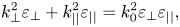
where k 0 = ω/c. If the plasma density is sufficiently low, the SW can propagate and fill the volume. More typically, the SW is evanescent and decays on the scale ${\delta _{\textrm{es}}}\sim {({m_e}/{m_i})^{1/2}}/{k_{||}}$ in the electrostatic limit, $k_0^2{\varepsilon _ \bot } \ll k_{||}^2$
 , and on the scale $\; {\delta _{\textrm{em}}}\sim c/{\omega _{\textrm{pe}}}$
 in the electromagnetic limit, $k_0^2{\varepsilon _ \bot } \gg k_{||}^2$
 . These scale lengths are very short, often only a few mm for plasma conditions where good antenna coupling is possible. If RF sheath rectification effects are only present from local RF fields on the limiter surface, then they too and the E × B convection they generate should be confined to relatively small distances from the antenna surface. Experimental observations (Van Nieuwenhove & Oost Reference Van Nieuwenhove and Oost1992; D'Ippolito et al. Reference D'Ippolito, Myra, Jacquinot and Bures1993; Gunn et al. Reference Gunn, Colas, Ekedahl, Faudot, Fuchs, Heuraux, Goniche, Kočan, Mendes, Ngadjeu, Petržílka, Saint-Laurent and Vulliez2008; Cziegler et al. Reference Cziegler, Terry, Wukitch, Garrett, Lau and Lin2012; Hong et al. Reference Hong, Wukitch, Lin, Terry, Cziegler, Reinke and Tynan2017) show that DC fields typically penetrate one or two cm radially, much larger than δ es or δ em. We will consider some physical mechanisms that can influence the penetration of sheath-induced potentials.

Figure 19. Schematic geometry in the radial (vertical) - toroidal (horizontal) plane. In this configuration penetration of RF-generated sheath fields either towards the main SOL or in the secondary SOL between the antenna and the limiter could be of interest.
One class of mechanisms involves nonlinear RF physics in the plasma volume, unrelated to sheath physics. If the SW fields are sufficiently strong, the ponderomotive force can expel plasma along the field lines away from the region of strongest intensity (Russell, Myra & D'Ippolito Reference Russell, Myra and D'Ippolito1998; Myra et al. Reference Myra, D'Ippolito, Russell, Berry, Jaeger and Carter2006; Van Eester & Kristel Reference Van Eester and Kristel2015). The plasma density may then be low enough to allow SW propagation in the depleted plasma channel, thereby increasing the radial penetration distance. In less extreme cases, the reduced density may increase δ em or allow the δ es estimate to apply. The condition for significant expulsion is that the ponderomotive potential ψp exceed the temperature. Expressions for the ponderomotive potential in fluid theory are given in Lee & Parks (Reference Lee and Parks1983) and Catto & Myra (Reference Catto and Myra1989). In order of magnitude ${\psi _p}\sim m{\tilde{v}^2}/2$ where m is the species mass (electrons or ions) and $\tilde{v}$
 is the species jitter velocity in the RF fields. For SW ICRF fields, the jitter velocity is dominated by ${\tilde{v}_{||}}$
 for electrons, and by ${\tilde{v}_ \bot }$
 for ions. Thus, the jitter velocity must be comparable to the thermal velocity for a large ponderomotive effect.
Even if RF nonlinearities in the volume do not directly cause increased radial penetration, interaction with the sheath can occur in several ways. One, already introduced in § 6.2, is propagation of a sheath plasma wave along the sheath surface of the limiter in figure 19. The sheath plasma wave can be strongly evanescent along B, moving away from the sheath surface, i.e. k || is imaginary, which permits a real k ⊥ in the SW dispersion relation and consequent radial penetration in a high-density plasma. The sheath–plasma wave is nothing more than a type of slow ‘surface’ wave that is enabled by the sheath BC. In order to have significant interaction of the antenna fields with a limiter, the limiter must be sufficiently close. In a simplified RF excitation model (Myra & D'Ippolito Reference Myra and D'Ippolito2010) the sheath interaction was found to be strong in dense plasmas (so that the SW is evanescent) when ${L_{||}} \ll {\delta _i}$ where L || is the magnetic connection length and ${\delta _i} = c/{\omega _{\textrm{pi}}}$
 is the ion skin depth. This condition is essentially a consequence of (6.29) which is roughly $k_ \bot ^2\delta _{\textrm{em}}^2 + k_{||}^2\delta _i^2 ={-} 1$
 in the ICRF and/or high harmonic fast wave (HHFW) regimes. The model does not account for a realistic antenna spectrum, and it is plausible that sheath excitation would occur for ${L_{||}}\; > {\delta _i}$
 if the antenna excites significant amplitudes for modes with ${k_{||}}{\delta _i}\; < 1$
 and specifically with ${k_{||}}{L_{||}}\sim 1$
 . A Green's function method for assessing the parallel proximity effect of antenna and wall with more realistic excitations is described in Colas et al. (Reference Colas, Lu, Křivská, Jacquot, Hillairet, Helou, Goniche, Heuraux and Faudot2017), but in this case it is difficult to extract a simple analytical scaling.
A separate RF sheath related effect, considered by Faudot et al. (Reference Faudot, Colas, Heuraux and Gunn2010) modifies the RF dispersion relation (6.29) and thereby changes the RF penetration depth perpendicular to B. On field lines that terminate on nearby sheaths where the magnetic connection length is short enough to apply the flute limit k || ≈ 0 in the plasma volume, one can integrate ∇⋅J = 0 along the field lines and employ the sheath current J || in place of the usual fluid response. That is, instead of ${J_{||}} = {\sigma _{||}}{E_{||}}$ with parallel conductivity ${\sigma _{||}} = \textrm{i}\omega {\varepsilon _0}\omega _{\textrm{pe}}^2/{\omega ^2}$
 one now has ${J_{||}} = {n_e}e{c_s}[1 - exp ( - e\varPhi /{T_e})] \to {n_e}{e^2}{c_s}\varPhi /{T_e}$
 upon linearization. The electrostatic dispersion relation is then ${k_ \bot }{J_ \bot } + 2i{J_{||}}/{L_{||}}$
 with ${J_ \bot } ={-} i{\sigma _ \bot }{k_ \bot }\varPhi ,{\sigma _ \bot } ={-} \textrm{i}\omega {\varepsilon _0}{\varepsilon _ \bot }$
 and with the usual ε ⊥ given following (3.2). The factor of 2 is from the two sheaths at the ends of a given field line. For a rough estimate relevant to ICRF ($\omega \sim {\varOmega _i}$
 but not too close to resonance and above the lower-hybrid density), one may take $\omega {\varepsilon _ \bot } = \omega _{\textrm{pi}}^2/{\varOmega _i}$
 . Using $k_ \bot ^2 \to - 1/L_ \bot ^2$
 the penetration depth is then estimated as
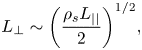
which is essentially the (Faudot et al. Reference Faudot, Colas, Heuraux and Gunn2010) result, except for ${\rho _s} \to {\rho _i}$ . The applicability of the flute approximation again requires a sufficiently small L || or a sufficient large excitation of low k || modes.
All of the mechanisms discussed so far are associated with the RF wave. There are also mechanisms that operate on the ‘DC’ time scale, i.e. the much slower time scale of plasma turbulence. The turbulent cross-field conductivity mentioned in the previous section as well as other mechanisms permitting perpendicular currents (such as the current from neutral–plasma friction) will act to increase radial penetration of DC or slow time scale electric fields from sheath rectification.
In D'Ippolito et al. (Reference D'Ippolito, Myra, Ryan, Righi, Heikkinen, Lamalle and Noterdaeme2002) an estimate of the radial penetration depth of ‘DC’ fields was made from the vorticity equation by balancing the nonlinear (low-frequency) ion polarization current with the parallel sheath current on field lines not directly connected to the antenna, but passing in front of it. (The term ‘DC’ is used loosely here because it is expected that strongly sheared RF potentials will result in Kelvin-Helmholtz instabilities and time-varying turbulence, which nevertheless will be low frequency compared with RF frequencies.) The vorticity equation is a statement of charge conservation $\boldsymbol{\nabla }\boldsymbol{\cdot }{\boldsymbol{J}_ \bot } ={-} {\nabla _{||}}{J_{||}}$ and the terms in question read

where the Boussinesq approximation has been made on the left-hand side (constant density in ω pi) and ${\boldsymbol{v}_E} = \boldsymbol{B} \times {\nabla _ \bot }\varPhi /{B^2}$ . Here, a slight departure from the notation of previous sections is made in that Φ is the upstream potential (previously denoted in the microscale model by Φ 0) because the macroscale plasma is now being considered.
As in (2.2) when Φ = (Te/e) ln μ (~3.18 for deuterium), there is no parallel current flow; otherwise, the circuit must be completed by ion polarization currents represented by the left-hand side of the equation. In the latter case the problem is necessarily two- (or three-) dimensional. For simplicity, we assume perpendicular incidence of the magnetic field as in figure 19. Estimating ${\nabla _{||}}\sim 1/{L_{||}}$ and ${\nabla _ \bot }\sim {\boldsymbol{e}_x}/{L_x} + {\boldsymbol{e}_y}/{L_y}$
 , where Lx and Ly are the radial and binormal (approximately poloidal) scale lengths of the potential, one obtains on the left-hand side $({\partial _t} + {\boldsymbol{v}_E}\boldsymbol{\cdot }{\nabla _ \bot })\nabla _ \bot ^2\Phi \sim {\Phi ^2}/(BL_x^3{L_y})$
 where the estimate assumes that ${\partial _t}\; < {\boldsymbol{v}_E}\boldsymbol{\cdot }{\nabla _ \bot }$
 and Lx < Ly. On the right-hand side we consider the case where just in front of the antenna the plasma potential is large and positive so that the parallel current is approximately the ion saturation current, necs. These rough approximations result in the order-of-magnitude convective cell penetration length estimate and scaling (D'Ippolito et al. Reference D'Ippolito, Myra, Ryan, Righi, Heikkinen, Lamalle and Noterdaeme2002)
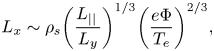
where ${\rho _s} = {c_s}/{\varOmega _i}$ . A slightly different scaling is obtained if Ly ~ Lx. Although (6.32) should capture the main qualitative scaling trends of this mechanism, the actual, likely turbulent, situation presents a formidable challenge for analytical estimates. This is due in part to the fact that turbulence by its very nature presents a range of time and space scales which are difficult to represent in simple estimates of the type presented here.
As of this writing, there is no single, generally accepted explanation for the experimentally observed radial penetration of the RF-induced sheath potential.
6.8. Impurity sputtering
As mentioned several times previously, one of the main deleterious effects of RF sheaths is the enhanced sputtering that results from ions being accelerated by the RF sheath electric field, and impacting the surface at energies much greater than thermal. In the high-frequency $\omega \gg {\omega _{\textrm{pi}}}$ ‘immobile-ion’ limit the inertia of the ions prevents them from responding to the RF oscillations but they are still accelerated into the wall by the rectified DC sheath electric field. On the other hand, in the low-frequency $\omega \ll {\omega _{\textrm{pi}}}$
 ‘mobile-ion’ limit the ions respond to the total instantaneous sheath electric field which oscillates about the DC field, being alternately larger and smaller during the RF cycle.
The implications of this for sputtering were addressed using a fluid sheath model (similar to NoFlu) and a prescribed mapping to kinetic ion distribution functions and then to energy dependent sputtering coefficients in Elias et al. (Reference Elias, Curreli, Jenkins, Myra and Wright2019). A recent extension calculates IEADs directly from PIC sheath simulations using the hPIC code (Elias et al. Reference Elias, Curreli, Jenkins and Myra2021). Results were also compared with the energy and angle obtained from the NoFlu model of § 4.1. It was shown that for mobile ions the IEAD has two ‘centres’: one corresponding to the low sheath voltage part of the RF cycle at low energy close to the magnetic field angle and another corresponding to the high sheath voltage part of the RF cycle at high energy and with an angle that is pushed more towards perpendicular incidence on the wall. For nearly grazing incidence magnetic fields or at high frequency $\omega \gg {\omega _{\textrm{pi}}}$ , the two centres coalesce as a result of increased ion inertia.
Integrated simulations taking into account RF propagation or evanescence at surfaces, RF sheaths, sputtering and subsequent transport of impurities are required for modelling experiments, and are being developed. Further discussion of this topic is beyond the scope of the present paper.
6.9. Other topics
6.9.1. Insulating coatings
Many experimental facilities have employed insulating coatings between the wall or antenna and the plasma to mitigate ICRF-induced sheaths. The idea stems from original work by Majeski et al. (Reference Majeski, Probert, Tanaka, Diebold, Breun, Doczy, Fonck, Hershkowitz, Intrator, McKee, Nonn, Pew and Sorensen1994). In the corresponding lumped circuit model, the sheath is in series with an insulator, as illustrated schematically in figure 20 (Myra et al. Reference Myra, D'Ippolito, Rice and Hazelton1997). The RF voltage divider so created results in only a fraction of the total RF voltage being dropped across the sheath; the rest appears across the insulator. This reduces the sheath voltage available for accelerating ions into the surface. Consequently, if the insulator has a high enough impedance relative to the sheath, sputtering can be greatly reduced. Unfortunately, so far it has not been possible to identify insulating materials that are compatible with fusion reactor requirements. The ideal material would be electrically insulating but have some thermal conductivity in order to tolerate the plasma heat load. Some promising exploratory work on a new class of composite insulators developed for this purpose are discussed in D'Ippolito et al. (Reference D'Ippolito, Myra, Rice and Hazelton1997).
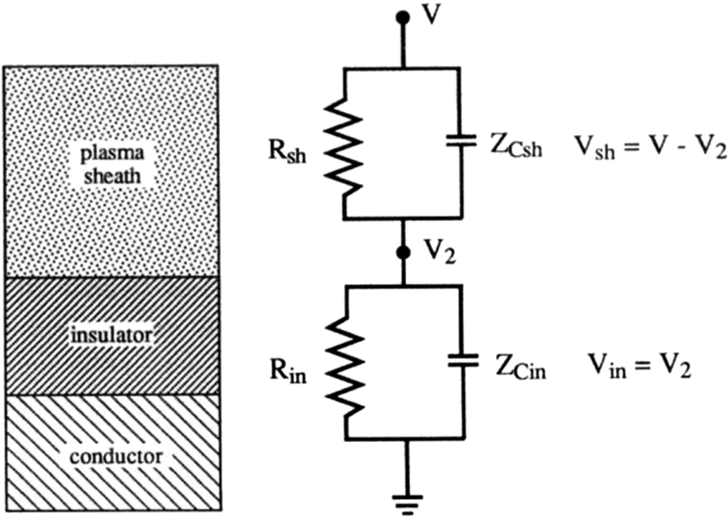
Figure 20. Circuit diagram illustrating the effect of an insulating coating in reducing the sheath voltage. Here, V is the total RF voltage at the sheath entrance, V sh and V in are the voltages appearing across the sheath and insulator respectively. In general both the sheath and insulator may have resistive and capacitive contributions to the impedances. Reprinted by permission from figure 1 of Myra et al. (Reference Myra, D'Ippolito, Rice and Hazelton1997).
6.9.2. Tangent and grazing magnetic fields
A number of modelling complications occur when the magnetic field grazes the surface at a small angle. This situation remains to be addressed in any comprehensive and complete way, even for static sheaths, let alone for biased RF sheaths. Nevertheless, the brief remarks here will expose some of the issues.
Physically, the sheath changes character when the magnetic field angle with the surface is sufficiently small that the electrons are no longer the species tending to have the largest particle flux into the surface (in the absence of a sheath potential). Estimating at the non-neutral sheath entrance where the Bohm condition is met, this condition happens when $|{b_n}|{v_{\textrm{te}}}\; < {c_s}$ . For smaller |bn| the sheath potential can reverse in order to confine the ions. At exact tangency, bn = 0, ions strike the wall by ‘scrape-off’ from finite gyro-radius effects and ion fluid motion perpendicular to B. These latter two effects are estimated to be in the ratio ρi/ρΦ where $\rho _\Phi ^2 \equiv e{\varPhi _{\textrm{sh}}}/({m_i}\Omega _i^2)$
 . However, without cross-field transport there would be no net flux of either species to a flat one-dimensional wall beyond an initial transient phase (Gerver, Parker & Theilhaber Reference Gerver, Parker and Theilhaber1990). It is expected that in this rather special situation, anomalous (e.g. turbulent) transport would control the structure of the sheath. Indeed, Kelvin–Helmholtz vortices played this role in corresponding simulations (Parker et al. Reference Parker, Xu, Lichtenberg and Birdsall1992). Because points where bn = 0 occupy a measure-zero set in a realistic fusion device geometry with curved boundary surfaces, it might be hoped that a careful treatment of these special points is not required in the modelling of RF sheaths. At present this is not yet clear.
Consider a case where the magnetic field component normal to the surface approaches bn = 0 as one moves along the surface. In the sheath BC, (5.2), the impedance z sh remains finite under the model of § 4. (The particle admittances ye and yi go to zero in the limiting case, but the capacitive contribution yd remains.) On the plasma side of the sheath the RF current directed into the plate is given by ${J_n} ={-} \textrm{i}\omega {\varepsilon _0}\boldsymbol{n}\boldsymbol{\cdot }\boldsymbol{\varepsilon }\boldsymbol{\cdot }\boldsymbol{E}$ where, as usual, n is the unit surface normal. For finite bn this is typically dominated by the term containing the large parallel dielectric $\boldsymbol{\varepsilon } \approx \boldsymbol{bb}{\varepsilon _{||}}$
 leaving ${J_n} \approx{-} \textrm{i}\omega {\varepsilon _0}{b_n}{\varepsilon _{||}}{E_{||}}$
 . Other contributions such as from ε ⊥E ⊥ are present but typically smaller until ${b_n}\sim {({m_e}/{m_i})^{1/2}}$
 as may be estimated from the electrostatic limit noting that ${E_ \bot }/{E_{||}}\sim {k_ \bot }/{k_{||}}\sim {({\varepsilon _{||}}/{\varepsilon _ \bot })^{1/2}}$
 . Thus, as ${b_n} \to 0$
 , Jn is reduced by nearly two orders of magnitude from its value when bn is of order unity. Mathematically, the sheath BC, ${\boldsymbol{E}_t} = {\nabla _t}({z_{\textrm{sh}}}{J_n})$
 with small Jn might be expected to reduce to the perfectly CW BC, Et = 0, which would seem benign. Unfortunately, numerical simulations (Kohno 2016) have shown that, at least under some conditions, a solution instead develops with finite Et and rapid oscillations in the tangential direction, i.e. as Jn becomes small, ∇t becomes large and the solution is difficult to resolve with reasonable numerical grids. This occurs because on a curved surface the changes in bn induce rapid and dramatic changes in Jn as one moves through the point where bn = 0. This helps to promote coupling of the incident RF branch (either FW or SW) to a short-scale-length sheath–plasma wave (Kohno, Myra & D'Ippolito Reference Kohno, Myra and D'Ippolito2013). A point which merits further investigation is whether a local sheath BC is appropriate near the tangency point since currents can flow along the surface coupling different points on the surface.
A second potential issue is that the Maxwell–Boltzmann electron model becomes invalid when ${v_{\textrm{te}}}\; < \omega {\Delta _{||}}$ where Δ || = Δ/bn; see (4.27). For small bn we are instead in the fluid electron limit, where electrons jitter in the RF fields: the force from E || is balanced by electron inertia. In intermediate cases ${v_{\textrm{te}}} \sim \omega {\Delta _{||}}$
 the electrons can gain energy from the fields, in analogy to Fermi acceleration or Landau resonance (Lieberman & Godyak Reference Lieberman and Godyak1998).
Calculations of the RF sheath impedance and rectification have not yet properly described these effects, and other complications that may arise in the grazing field line limit. A complete and rigorous treatment of this problem seems out of reach at present; it may be satisfactory to simply ascertain from experiments or simulations the level of rigor that is required for practical modelling applications.
6.9.3. Low power loading
An interesting but somewhat offbeat phenomenon that was analysed theoretically (D'Ippolito & Myra Reference D'Ippolito and Myra1996) and observed experimentally (Swain et al. Reference Swain, Pinsker, Baity, Carter, deGrassie, Doyle, Hanson, Kim, Moyer and Petty1997) is that of sheath effects on the loading (or coupling) resistance of an ICRF antenna at very low powers. The topic is mentioned here for two reasons: it may provide a useful and direct experimental means of assessing antenna designs with respect to RF sheaths; and the experimental signature may be confused with density pump out by RF-driven convection or ponderomotive force.
The antenna loading resistance is a routinely measure quantity related to the RF power by

where ${P_{\textrm{rf}}} = {P_{\textrm{rad}}} + {P_{\textrm{sh}}}$ , ${P_{\textrm{rad}}}$
 is the RF power radiated by the antenna into the plasma, P sh is the power dissipated in near-field antenna sheaths, V ant is the antenna voltage and Z 0 is the antenna impedance. Although P rad depends on local plasma conditions such as the plasma density profile in front of the antenna, its voltage scaling is ${P_{\textrm{rad}}} \propto V_{\textrm{ant}}^2$
 . Thus, in the absence of sheath power dissipation or nonlinear density modification effects, RL is independent of V ant or RF power.
In the original description of low power loading (D'Ippolito & Myra Reference D'Ippolito and Myra1996), using the capacitive sheath model in the immobile-ion limit, the sheath power loss was taken to be the ion particle flux times the rectified sheath potential, ${P_{\textrm{sh}}} = Ze{n_i}{c_s}\langle {\varPhi _{\textrm{sh}}}\rangle$ . The rectified sheath potential is an order-unity fraction of the peak RF potential $|{\tilde{\varPhi }_{\rm sh}}|$
 driving the sheath, and that quantity in turn is proportional to the peak RF antenna voltage V ant. Thus, at low enough V ant, i.e. power, the sheath power losses dominate, ${P_{\textrm{rf}}} \approx {P_{\textrm{sh}}} \propto {V_{\textrm{ant}}}$
 and the loading scales as ${R_L} \propto 1/{V_{\textrm{ant}}}$
 .
.
To explore this in a bit more generality, recall from (6.14) that the RF power dissipated in the sheath is ${P_{\textrm{sh}}}/A = Re \hspace{0.5mm} {y_{\textrm{sh}}}|{\varPhi _{\textrm{sh}}}{|^2}/2$ which at first sight appears to scale like $|{\varPhi _{\textrm{sh}}}{|^2}$
 ; however, this does not account for the dependence buried in y sh. From (4.22) the real part of the admittance (which is dominated by the electrons) is proportional to $1/\xi = {T_e}/(e|{\tilde{\Phi }_{\textrm{sh}}}|)$
 . This recovers the scaling ${P_{\textrm{sh}}}\mathrm{\ \propto |}{\tilde{\Phi }_{\textrm{sh}}}|\propto {V_{\textrm{ant}}}$
 and ${R_L} \propto 1/{V_{\textrm{ant}}}$
 .
.
The predicted behaviour in RL due to sheath loading was observed in ICRF experiments on DIII-D below powers of approximately 100 kW, with a doubling of RL occurring at approximately 20 kW (Swain et al. Reference Swain, Pinsker, Baity, Carter, deGrassie, Doyle, Hanson, Kim, Moyer and Petty1997). It follows that at very high powers (${\gg} 100\;\textrm{kW}$ for this antenna) the fractional power lost to near-field antenna sheaths should be small in total. Nevertheless, sheath power dissipation is of considerable significance since that power is often deposited in localized spots on antenna surfaces vulnerable to damage.
From the preceding mechanism we expect the loading to drop as ICRF power is ramped up. Other nonlinear mechanisms may also influence the loading and produce a similar signature. For example, the ponderomotive force can expel plasma from a small region in front of the antenna if the antenna excites strong electric fields with the SW polarization; see § 6.7 and references therein. Also, RF sheath-driven convection can modify the density in front of the antenna; see § 6.5. The pondermotive density depletion effect should scale as $V_{ant}^2$ while sheath-driven convection velocity should have a V ant scaling. The net effect on density at the antenna and the resulting loading is less clear.
Although low power loading has not received much attention since its recognition more than 20 years ago, it remains as a potentially useful diagnostic tool for comparing near-field sheaths with different antenna designs.
7. Conclusion
As should be evident from this tutorial, RF sheaths offer an environment which is exceedingly rich in physical content. No doubt future research will improve quantitative modelling and explore new aspects of RF sheaths that go well beyond the state of the art today. Topics that have not been touched upon, or barely touched upon, in this tutorial include sheaths for which the sheath electrons are only partially magnetized (of interest for low magnetic field laboratory experiments), multi-species ion effects, collisional RF sheaths, situations in which surface interactions contribute to the sheath structure (such as electron emission or sputtering avalanche), kinetic electron effects in the inertial and stochastic regimes, the complex topic of grazing angle sheaths and RF-driven arcs.
The most essential topics covered in this tutorial, not counting the introductory material in the first three sections, are the basic microscale sheath model of § 4.1, the sheath BC of § 5.1 and the macroscale RF sheath effects in §§ 6.1–6.5.
With regard to ICRF modelling, it will be beneficial to determine a somewhat minimalist and practical approach which is nonetheless sufficient to answer the most important questions and, importantly, suggest means by which the detrimental effects of ICRF surface interactions can be mitigated. Innovations in antenna design and operation, such as optimal phasing, power split between current straps, and field alignment of components have already resulted in dramatic improvements in ICRF operation. Arguably on specific machines and for specific operational scenarios ICRF-boundary interactions may be regarded as a solved problem. However, that is not to say that ICRF-edge modelling has matured to the point where it can both understand and quantify the detrimental ICRF issues of the past and confidently predict future behaviours under edge plasma conditions as yet largely unknown in ITER or a future demo device.
The modelling and control of RF sheath effects in tokamaks will likely require an integrated whole device approach much broader in scope than covered in this paper. In addition to the sheath physics covered here, it would include realistic electromagnetic modelling of complex three-dimensional antenna structures embedded in edge plasmas which themselves should be modelled self-consistently with the presence of RF. This would involve simulation of RF-driven convection, and an assessment of RF ponderomotive effects in a thin plasma region next to the antenna. Realistic modelling of both core absorption and edge and SOL (e.g. coaxial) mode propagation would need to be included. RF scattering by turbulence and the effects of RF-driven potentials on edge turbulence may play a role. The problem of global DC circuits may have to be assessed and treated in some fashion. Many of the individual pieces of these interactions are known or under development (Heuraux et al. Reference Heuraux, da Silva, Ribeiro, Despres, Campos Pinto, Jacquot, Faudot, Wengerowsky, Colas and Lu2015; Bonoli et al. Reference Bonoli and Green2020; Zhang et al. Reference Zhang, Bilato, Bobkov, Cathey, Di Siena, Hoelzl, Messiaen, Myra, Suárez López, Tierens, Usoltceva and Wright2021). It remains to assemble a practical high-fidelity integrated model. That task will present a significant challenge and opportunity for the ICRF fusion modelling community.
Acknowledgements
Discussions with D. A. D'Ippolito, H. Kohno, D. Smithe, T. Jenkins, D. Curreli, M. Elias, C. Lau, M. V. Umanksy, B. Van Compernolle, S. Vincena, J. Wright and members of the RF SciDAC project (Discovery through Advanced Computing Initiative: Center for Integrated Simulation of Fusion Relevant RF Actuators) over the entire course of the research are gratefully acknowledged. The author is especially grateful to the following colleagues for providing helpful suggestions for improving the manuscript: M. Elias, D. Green, H. Kohno, C. Lau, C. Migliore, M. Umansky and the anonymous referees. This paper is dedicated to the author's long time RF sheath physics collaborator, colleague and friend, the late D. A. D'Ippolito.
Editor William Dorland thanks the referees for their advice in evaluating this article.
Funding
This material is based upon work supported by the U.S. Department of Energy Office of Science, Office of Fusion Energy Sciences under Award Numbers DE-AC05-00OR22725 sub-contract 4000158507 and DE-FG02-97ER54392. The latter award funded some portions of the original material summarized here.
Declaration of interests
The author reports no conflict of interest.
Appendix A. Table of notations
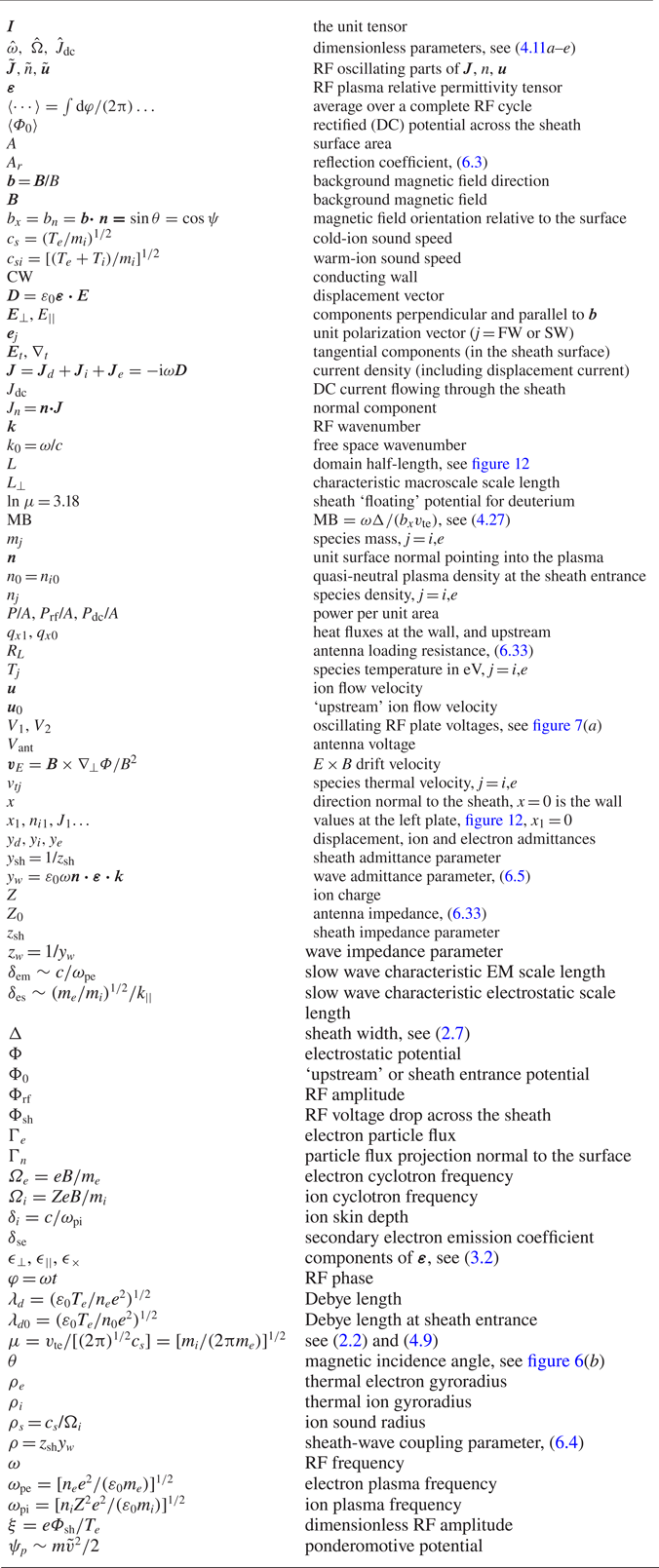
Appendix B. Table of acronyms