


1. Introduction
Recent years have seen a marked increase in large-scale destructive wildfires in many regions, including North America, Siberia, Australia and Europe. This is consistent with the study of Jolly et al. (Reference Jolly, Cochrane, Freeborn, Holden, Brown, Williamson and Bowman2015), who use an annual metric measuring ‘fire weather’ season length to show an 18.7 % increase in global mean fire weather season length over the period 1979 to 2013. The 2021 Intergovernmental Panel on Climate Change (IPCC) report (Masson-Delmotte et al. Reference Masson-Delmotte2021) predicts further increases of fire weather conditions. Understanding the dynamics of wildfires is therefore becoming increasingly vital. From a fluid mechanics perspective, wildfires are complex, involving physical, chemical and thermodynamic processes, and their interaction with environmental factors such as winds, vegetation and topography. A variety of approaches aimed at understanding wildfires have been adopted, including empirical, statistical and physical modelling, with methods spanning experimental, observational, mathematical and computational techniques. Many of these previous works are summarised in the review articles of Perry (Reference Perry1998), Pastor et al. (Reference Pastor, Zárate, Planas and Arnaldos2003), Sullivan (Reference Sullivan2009a,Reference Sullivanb,Reference Sullivanc) and Bakhshaii & Johnson (Reference Bakhshaii and Johnson2019).
Minimising the risks and impacts of wildfires requires predicting the behaviour of the spreading fire line. In this work, the fire line is taken to be the interface between burned and unburned regions, and how this interface evolves on a two-dimensional surface – the land surface – is a key question. Mathematically, the problem is the geometric evolution of a two-dimensional non-intersecting curve in which the normal velocity at a point on the curve is either prescribed or needs to be determined according to a physical model for the fire line evolution.
An essential ingredient to wildfire spread is the availability of oxygen. The processes and effects in which oxygen additional to that otherwise available in calm conditions is fed to the fire by fire-induced wind (the ‘fire wind’, also known as pyrogenic wind/flow, see Hilton et al. Reference Hilton, Sullivan, Swedosh, Sharples and Thomas2018) are the subject of this study. Buoyant upflow over the burned region creates local low pressure, which in turn acts as a sink, drawing in surrounding air in a shallow ground-level layer and so generating fire wind (Smith, Morton & Leslie Reference Smith, Morton and Leslie1975). Beer (Reference Beer1991) presents a stoichiometric argument that the oxygen necessary for combustion must be supplied by turbulent mixing from an inward horizontal flow. In calm conditions, this requirement leads to the generation of fire wind. It is interesting to note that Beer (Reference Beer1991) also shows that when an ambient wind is present (which the present study does not consider), it will supply the sufficient oxygen needed for combustion, so there is little reason to expect fire wind in the case of a wind-driven fire. However, fire winds of velocities up to 3 m s $^{-1}$ have been observed for even modest-sized ( $\approx 2$ km radius in the horizontal direction) wildfires (e.g. Lareau & Clements Reference Lareau and Clements2017). In their numerical simulation of the 1991 Oakland Hills fire, Trelles & Pagni (Reference Trelles and Pagni1997) found that the fire wind rapidly increased from $2.6\ {\rm m~s}^{-1}$ to $13.0\ {\rm m~s}^{-1}$ as the fire intensified. Moreover, they found that the horizontal fire-induced wind was drawn towards the centroid of multiple fire plumes.
This paper formulates a simple two-dimensional model for the effect of fire wind on wildfires, which is used to investigate fire line stability and its nonlinear evolution. The model assumes that the oxygen concentration in the unbounded region exterior to the fire is governed by the steady advection–diffusion equation, with advective transport effected by the fire wind. This fire wind, modelled by a two-dimensional potential flow, brings in oxygen-rich air from infinity for consumption by the fire at the fire line. In response, the fire line velocity is proportional to the normal gradient of oxygen at the fire line, in the direction of its outward normal. As such, the fire line is susceptible to the Mullins–Sekerka instability (Mullins & Sekerka Reference Mullins and Sekerka1964) and, as will be shown, may develop finger-like protrusions.
The steady two-dimensional advection–diffusion equation and Laplace equation, which govern the oxygen transport and fluid flow, respectively, are a pair of conformally invariant partial differential equations (PDEs) (Cummings et al. Reference Cummings, Hohlov, Howison and Kornev1999; Bazant Reference Bazant2004) – a property that is exploited in the numerical method. The infinite unburned region, with boundary representing the fire line, is represented as a conformal map from the unit disk in some ‘mathematical’ plane. The free-boundary problem for the unknown fire line then becomes that of determining the conformal map using a Polubarinova–Galin type equation (Gustafsson & Vasil'ev Reference Gustafsson and Vasil'ev2006). Similar approaches have been used in both the analytical and numerical solutions of Hele-Shaw free-boundary problems (e.g. Howison Reference Howison1986; Dallaston & McCue Reference Dallaston and McCue2013; Miranda & Widom Reference Miranda and Widom1998) and determining the evolution of two-dimensional freezing, melting or dissolution of bodies in two-dimensional potential flows (e.g. Cummings et al. Reference Cummings, Hohlov, Howison and Kornev1999; Rycroft & Bazant Reference Rycroft and Bazant2016; Ladd, Yu & Szymczak Reference Ladd, Yu and Szymczak2020).
Fire lines have been observed to develop ‘fingering’ instabilities. Clark et al. (Reference Clark, Jenkins, Coen and Packham1996a) discuss the 1985 Onion sage brush fire in Owens Valley, California, where the fire line developed multiple protrusions spaced about 1 km apart (see their figure 1). Clark et al. (Reference Clark, Jenkins, Coen and Packham1996a) used a three-dimensional coupled fire-atmosphere numerical model to attribute finger formation to feedback between the hot convective plume and the near-surface convergence at the fire line. However, there is no oxygen effect in their simulations, and the fingering mechanism is owing to vorticity generation and the breakup of the buoyancy-driven plume into smaller cells (see also Clark et al. Reference Clark, Jenkins, Coen and Packham1996b). Dold, Sivashinsky & Weber (Reference Dold, Sivashinsky and Weber2005) also propose a dynamic model for fire line instability linked to the presence of a hot plume over the fire. The plume partially blocks incoming airflow and, along with a stably stratified atmosphere, the overall effect is to accelerate incoming air in the direction normal to the fire line. They use a stability analysis to argue that perturbations to the fire line grow owing to an increased airflow, hence increased burning rate, at the more advanced parts of the front. Although not mentioned explicitly, the Dold et al. (Reference Dold, Sivashinsky and Weber2005) assumption that the burn rate, or fire line speed, is proportional to the oncoming airflow feeding the fire appears analogous to the oxygen effect considered in this paper. Recently, Quaife & Speer (Reference Quaife and Speer2021) used a two-dimensional, reduced physics, cellular automata model of fire-atmosphere interaction incorporating a fire-plume-induced convective sink, and vorticity sources at the flanks of the fire. Amongst a variety of fire line behaviours observed in their model was fingering, in the form of the breakup of the fire line into multiple advancing heads.
Previous works that consider explicitly the effects of oxygen transport in producing fingering instability in combustion are the experimental investigations by Zik, Olami & Moses (Reference Zik, Olami and Moses1998) and Zik & Moses (Reference Zik and Moses1999), and the numerical work of Conti & Marconi (Reference Conti and Marconi2002, Reference Conti and Marconi2010). The former describe experiments in which solid fuel in a Hele-Shaw cell is forced to burn against an oxidising wind. A fingering instability is observed with two decoupled length scales: the finger width and the inter-finger distance, the latter being determined by the Péclet number measuring the relative importance of oxygen and diffusion. Motivated by these experiments, Kagan & Sivashinsky (Reference Kagan and Sivashinsky2008) derive a nonlinear PDE that models the free boundary between the solid fuel and air, demonstrating that the fingering is similar to the instability occurring in premixed gas flames. Conti & Marconi (Reference Conti and Marconi2002, Reference Conti and Marconi2010) use a numerical lattice model to consider the diffusion of both heat and oxygen at advancing fire fronts. Fingering is observed, with the nonlinear evolution of the front developing into either a cellular or a dendritic pattern, depending on the parameters chosen, e.g. the initial oxygen concentration.
The structure of this paper is as follows. In § 2, the simplified model of fire line growth, incorporating the effects of oxygen advection and diffusion, is formulated for radial fires. The fire burns on a flat surface with uniform combustible fuel that, typically, is some form of vegetation, e.g. grass or heathland. The only wind present is the self-induced fire wind. In addition to the oxygen effect, the fire line velocity is assumed to have two other contributions. The first is a constant fire line velocity owing to the cumulative effect of radiation and convection. Determining fire line velocity from these effects alone is in itself a complex and difficult problem, with the comparative roles of convection and radiation still an active area of research (e.g. Finney et al. Reference Finney, Cohen, Forthofer, McAllister, Gollner, Gorham, Saito, Akafuah, Adam and English2015). Here, following e.g. Hilton et al. (Reference Hilton, Miller, Sharples and Sullivan2016, Reference Hilton, Sullivan, Swedosh, Sharples and Thomas2018), it is assumed simply that radiation and convection, together with fuel type and the background level of oxygen, give rise to a constant fire line velocity  $v_0$ (the ‘rate of spread’, or ROS) in a direction normal to the fire line. The second contribution is the effect of the curvature of the fire line: curvature acts to increase the propagation of concave regions of the fire line, since more heat is able to be transferred into such unburned regions. This causes faster ignition of the fuel compared to regions outside of convex fire line segments, which transfer heat to a wider, and so larger, area of unburned fuel (Markstein Reference Markstein1951; Sethian Reference Sethian1985; Sharples et al. Reference Sharples, Towers, Wheeler, Wheeler and McCoy2013; Wheeler et al. Reference Wheeler, Wheeler, McCoy and Sharples2015; Hilton et al. Reference Hilton, Miller, Sharples and Sullivan2016). Consequently, curvature stabilises, or smooths out, perturbations, in this sense acting in the same way as ‘curve-shortening’ (Gage & Hamilton Reference Gage and Hamilton1986; Grayson Reference Grayson1987; Dallaston & McCue Reference Dallaston and McCue2016).
The linear stability of the fire line is investigated in § 3, quantifying its dependence on wavenumber, ROS, curvature and the Péclet number. Nonlinear evolution, including finger formation, of perturbed circular fire lines is then computed numerically using the conformal mapping approach in § 4, along with a derivation of a law for the rate of change of area of the burned region, which serves as a useful check on the numerical results. Periodic planar fire lines are considered in § 5; this is analogous to studying a large wildfire at a local scale. Finally, § 6 provides a discussion of the results obtained from this paper and their application to wildfires.
2. Radial fire model
The radial wildfire problem is illustrated in figure 1, where figure 1(a) gives a top-down (plan) view of the wildfire, and 1(b) gives a side view. Consider a two-dimensional, non-overlapping, finite curve  $\gamma$ – the fire line – enclosing a region $R$ of burned fuel, where the unburned region $\varOmega$ is the $(x,y)$-plane punctured by $R$, and the fire line is traversed with $R$ on the left. It is assumed that a single bone-dry fuel type is used, distributed uniformly on flat terrain with zero ambient wind; the only wind present is a self-induced ‘pyrogenic (fire) wind’. Smith et al. (Reference Smith, Morton and Leslie1975) discuss in detail the role of dynamic pressure in generating this fire wind; using a numerical model, they show that the strong buoyant acceleration over the fire region generates locally low pressure, leading to a horizontal pressure gradient that in turn generates the pyrogenic wind (Hilton et al. Reference Hilton, Sullivan, Swedosh, Sharples and Thomas2018). This strong inflow is quite different in nature to the relatively weak, entraining inflows associated commonly with turbulent plume dynamics, and is best modelled using dynamic pressure, which communicates the effect of fire-driven buoyant air to the surrounding fluid. Pressure anomalies to model fire-driven surface winds have been used previously (e.g. Achtemeier Reference Achtemeier2012). Once the fire wind reaches the fire line, a proportion of its oxygen is used in combustion (Beer Reference Beer1991) before the air enters the burned region and is ejected from the system.

Figure 1. The radial wildfire model: (a) plan view; (b) side view. The blue arrows represent the direction of the fire wind governed by the potential  $\phi$.
It is assumed that the fire wind is a two-dimensional horizontal flow occurring in a shallow layer of depth  $H$ in the unburned region $\varOmega$ parallel to the ground surface; see figure 1(b). The layer depth $H$ is much smaller than the horizontal length scale of the fire. Defining the Reynolds number $Re=UH/D$, where $U$ is a typical fire wind velocity at the fire line and $D$ is the momentum diffusivity for turbulent flow, and using values typical for a small starting fire – $U\sim 0.025\ {\rm m~s}^{-1}$, $H\sim 10{\rm m}$ and $D\sim 1\ {\rm m}^{2}\ {\rm s}^{-1}$ (Bebieva et al. Reference Bebieva, Oliveto, Quaife, Skowronski, Heilman and Speer2020) – gives $Re\approx 0.25$. Thus, to a reasonable approximation, the Stokes flow equations govern the flow in the shallow layer exterior to the fire. This approximation ‘improves’ further from the fire where the inflow velocity decreases. However, as the fire intensifies, the velocity scale $U$ will increase, leading to an increase in $Re$, but this increase may be offset due to an expected increase in the diffusion coefficient $D$, owing to increased turbulent mixing. Assuming that the approximation remains reasonable, such shallow flows are analogous to those in a Hele-Shaw cell, and a standard derivation involving integration of the Stokes equations over the layer depth (see e.g. Gustafsson & Vasil'ev Reference Gustafsson and Vasil'ev2006) shows that $\boldsymbol {u}=\boldsymbol {\nabla }\phi \sim -\boldsymbol {\nabla }p$, where the velocity potential $\phi$ is proportional to the (negative) pressure $p$. Note that $\boldsymbol {u}$ is the average fire wind velocity over $H$. Without loss of generality, in the present work, the low pressure over the fire is represented by taking $\phi =0$ over the fire, and on $\gamma$ in particular.
The fluid is incompressible and, to good agreement with experimental data (Hilton et al. Reference Hilton, Sullivan, Swedosh, Sharples and Thomas2018), the wind can also be treated as irrotational, so  $\phi$ satisfies the Laplace equation
 \begin{equation} \nabla^{2}\phi=0\quad \text{in}\ \varOmega.\end{equation}
Irrespective of the assumptions made here, modelling the flow exterior to wildfires and plumes using solutions of the two-dimensional Laplace equation has been used previously by e.g. Weihs & Small (Reference Weihs and Small1986), Maynard, Princevac & Weise (Reference Maynard, Princevac and Weise2016), Sharples & Hilton (Reference Sharples and Hilton2020), Quaife & Speer (Reference Quaife and Speer2021) and Kaye & Linden (Reference Kaye and Linden2004).
Further, it is assumed that the fire wind velocity  $\boldsymbol {u}$ is much larger than the normal velocity $v_n$ of the fire line, so the system is quasi-steady. The oxygen concentration $c$ thus satisfies the steady advection–diffusion equation
 \begin{equation} \boldsymbol{u}\boldsymbol{\cdot}\boldsymbol{\nabla} c=D\,\nabla^{2} c\quad \text{in}\ \varOmega, \end{equation}
where  $D$ is the diffusivity of $c$. Equations (2.1) and (2.2) form a coupled system to be solved, with suitable boundary and far-field conditions needed.
The background oxygen concentration far from the fire,  $r\to \infty$, is denoted $c=c_{\infty }$, and is $c=c_f$ on the fire line $\gamma$ itself. This latter condition results from an assumption that the fire is uniform in its intensity at points around the fire line, and consumes oxygen to the same level; the actual value of $c_f< c_\infty$ is immaterial. Specification of such a Dirichlet boundary condition on the moving interface for the quantity undergoing advection and diffusion is used in other moving-boundary problems, e.g. in Cummings et al. (Reference Cummings, Hohlov, Howison and Kornev1999) and Tsai & Wettlaufer (Reference Tsai and Wettlaufer2007).
The low pressure at the fire plume appears as an effective sink in the far field, so the velocity potential has behaviour  $\phi =-(Q/2{\rm \pi} )\log {r}$ in the far-field, where $Q>0$ is the strength of the sink. Note that as the fire expands and intensifies over time, the ability of the fire plume to draw in surrounding air increases, thus the sink strength $Q$ also increases over time, leading to a larger fire wind flux (Trelles & Pagni Reference Trelles and Pagni1997). Therefore, let $Q=Q(t)=Q_0\,q(t)$, where $q(0)=1$, and $Q_0$ is some constant. The implications of this are considered further throughout this paper. To summarise, the boundary and far-field conditions for the velocity potential $\phi$ and the oxygen concentration $c$ are
 \begin{gather} c=c_f,\quad \phi=0\quad \text{on}\ \gamma, \end{gather}
 \begin{gather}c\rightarrow c_\infty,\quad \phi\rightarrow-\frac{Q(t)}{2{\rm \pi}}\log{r}\quad \text{as}\ r\rightarrow\infty. \end{gather}
 The velocity  $v_n$ of the fire line $\gamma$ in the direction of the outward unit normal $\hat {\boldsymbol {n}}$ is sought. Markstein (Reference Markstein1951) first proposed a simple model for the velocity $v_n$ of flame fronts, which showed qualitatively good agreement with experimental data. The model reads as
 \begin{equation} v_n = v_0 - \delta\kappa. \end{equation}
The constant  $v_0$ is the basic rate of spread (ROS), a parameter quantifying the physical properties of the fuel, e.g. the speed at which fuel ignites under heating, and the heat transferred by radiation and convection from burning to unburned fuel cells. While there is ongoing research in quantifying $v_0$ for different fuel types (Sullivan Reference Sullivan2009a; Finney et al. Reference Finney, Cohen, Forthofer, McAllister, Gollner, Gorham, Saito, Akafuah, Adam and English2015), $v_0$ is treated simply as some constant here. Markstein (Reference Markstein1951) found that the correction term $-\delta \kappa$ was needed for better matching with experimental results, where $\kappa$ is the (signed) curvature, and $\delta$ is a constant, with $\delta \ll v_0$. Note that (2.5) is a type of curve-shortening (or in this context curve-lengthening) equation (e.g. Grayson Reference Grayson1987; Dallaston & McCue Reference Dallaston and McCue2016). Physically, (2.5) acts to smooth out perturbations in the fire line; concave sections of the fire line grow faster as more heat is transferred to the unburned regions of fuel that these sections enclose. The geometric wildfire model (2.5) has been studied previously by e.g. Sethian (Reference Sethian1985) and Sharples et al. (Reference Sharples, Towers, Wheeler, Wheeler and McCoy2013); the latter simulated successfully the propagation of fire junctions using the model.
The purely geometric rule (2.5) does not lead to the sometimes observed phenomenon of wildfire fingering (Clark et al. Reference Clark, Jenkins, Coen and Packham1996a,Reference Clark, Jenkins, Coen and Packhamb; Dold et al. Reference Dold, Sivashinsky and Weber2005). Therefore, a dynamical oxygen effect is introduced into  $v_n$ in which the interface velocity is dependent on the gradient of $c$ in the normal direction, i.e. $v_n=\partial c/\partial n$. This additional term simulates the expected behaviour: the fire grows preferentially in the direction of higher oxygen concentration (the closer the fire line is to the source of oxygen, the more quickly combustion can occur and hence the faster the fire line propagates), which can result in fire fingering. In particular, the equation for $v_n$ is written as
 \begin{equation} v_n = v_0 -\delta\kappa+\alpha\hat{\boldsymbol{n}}\boldsymbol{\cdot}\boldsymbol{\nabla}c\quad \text{on}\ \gamma,\end{equation}
where  $\alpha$ is some constant. Whilst $v_0$ is a constant and the curvature $\kappa$ is a geometrical property of the fire line, $\hat {\boldsymbol {n}}\boldsymbol {\cdot }\boldsymbol {\nabla }c$ is dynamical and requires the solution for the oxygen concentration $c$. This is found by solving the system (2.1)–(2.4a,b).
2.1. Non-dimensionalisation and the Péclet number
The system (2.1)–(2.4a,b) and (2.6) is now non-dimensionalised. First, the length scale  $L$ is chosen to be the initial radius $L=R_0$ of the wildfire. Scalings are then chosen to give rise to an ${O}(1)$ oxygen-driven contribution to $v_n$, since oxygen effects are of particular interest in this study. Thus the dimensionless (starred) variables are
 \begin{equation} \boldsymbol{\nabla} = \frac{1}{L}\,\boldsymbol{\nabla}^{{\ast}},\quad \phi = \frac{Q}{2{\rm \pi}}\,\phi^{{\ast}},\quad c^{{\ast}}=\frac{c-c_f}{c_\infty-c_f},\quad t = \frac{L}{U\,\textit{Pe}_0}\,t^{{\ast}},\quad U=\frac{\alpha(c_\infty-c_f)}{L}, \end{equation}
where  $\textit {Pe}_0=Q_0/2{\rm \pi} D$, for $Q_0=Q(0)$, is the constant initial value of the Péclet number. The non-dimensional system for the wildfire problem, after dropping the stars, is
 \begin{gather} \textit{Pe}_0\,v_n=V_0 -\bar{\epsilon}\kappa+\hat{\boldsymbol{n}}\boldsymbol{\cdot}\boldsymbol{\nabla}c\quad \text{on}\ \gamma, \end{gather}
 \begin{gather}\nabla^{2}\phi=0\quad \text{in}\ \varOmega, \end{gather}
 \begin{gather}\textit{Pe}\,\boldsymbol{u}\boldsymbol{\cdot}\boldsymbol{\nabla} c= \nabla^{2} c \quad \text{in}\ \varOmega, \end{gather}
 \begin{gather}c=0,\quad \phi=0\quad \text{on}\ \gamma, \end{gather}
 \begin{gather}c\rightarrow 1,\quad \phi\rightarrow-\log{r}\quad \text{as}\ r\rightarrow\infty. \end{gather}
where the new dimensionless constants  $V_0$ and $\bar {\epsilon }$, representing the ROS and magnitude of the curvature effect, respectively, are
 \begin{equation} V_0 = \frac{Lv_0}{\alpha(c_\infty-c_f)},\quad \bar{\epsilon}=\frac{\delta}{\alpha(c_\infty-c_f)}. \end{equation}
 Note that the non-dimensional time-varying, Péclet number  $\textit {Pe}$ now appears in (2.10) and is
 \begin{equation} \textit{Pe} = \frac{Q(t)}{2{\rm \pi} D}=\frac{Q_0\,q(t)}{2{\rm \pi} D}=\textit{Pe}_0\,\,q(t). \end{equation}
Recall that the plume strength  $Q(t)=Q_0\,q(t)$ is assumed to grow in time as the fire expands, thus the Péclet number also increases in time. Choosing $q(t)\sim R(t)$, where $R(t)$ is the radius of the burned region $R$, gives
 \begin{equation} \textit{Pe}=\frac{\textit{Pe}_0}{R_0}\,R(t). \end{equation}
For all numerical experiments reported here,  $R_0=1$, so the Péclet number is simply $\textit {Pe}=\textit {Pe}_0\,R(t)$. Note also that $\textit {Pe}_0$ has been incorporated in the scale for time $t^{\ast }$ in (2.7a–e).
Finally, note that it is required on physical grounds that the fire always progresses from the burned region  $R$ into the unburned region $\varOmega$; this is known as the entropy condition (Sethian Reference Sethian1985). There is no explicit mechanism in the wildfire model (2.9)–(2.12) to enforce this entropy condition. This does not affect the linear stability results of § 3, since the fire line does not move, but such unphysical behaviour is possible in the nonlinear evolution of the fire line computed in § 4. In practice, this is likely to be rare, since both the $V_0$ and $\hat {\boldsymbol {n}}\boldsymbol {\cdot }\boldsymbol {\nabla }c$ terms cause the fire line to propagate towards the unburned region, and $\bar {\epsilon }$ is taken to be small in comparison since, as you may recall, $\delta \ll v_0$ and hence $\bar {\epsilon }\ll V_0$.
3. Stability analysis
The stability of a perturbed curve  $\gamma$ evolving under the system (2.8)–(2.12) is studied. Such stability is determined by the competing effects of curvature (stabilising) and oxygen consumption (destabilising), quantified by the parameters $\bar {\epsilon }$ and $\textit {Pe}$, respectively. It is expected that there is some range of wavenumbers that grow over time, hence are unstable, for certain choices of $\bar {\epsilon }$ and $\textit {Pe}$.
First, consider an unperturbed base state  $\gamma$ given by the circle $r=R(t)$, with $R(0)=1$, so that $\textit {Pe}=\textit {Pe}_0\,R(t)$. The solution to (2.9)–(2.12) is
 \begin{equation} \phi(r) ={-}\log{\frac{r}{R}},\quad c(r) = 1-\left(\frac{R}{r}\right)^{\textit{Pe}}. \end{equation}
 Since the curvature for a circle of radius  $R$ is $\kappa =R^{-1}$, (2.8) gives the normal velocity of $\gamma$ as
 \begin{equation} \textit{Pe}_0\,v_n = \textit{Pe}_0\,\dot{R}=V_0-\frac{\bar{\epsilon}}{R}+\frac{\textit{Pe}}{R}, \end{equation}
where the dot denotes the time derivative. Dividing through by  $\textit {Pe}$ gives the relative growth of radius $R$:
$R$:
 \begin{equation} \frac{\dot{R}}{R}=\frac{V_0}{\textit{Pe}_0\,R}-\frac{\sigma}{R}+\frac{1}{R}=\frac{1}{R} \left[\frac{V_0}{\textit{Pe}_0}-\sigma+1\right], \end{equation}
where  $\sigma =\sigma (t)=\bar {\epsilon }/\textit {Pe}$. Therefore, provided that $\bar {\epsilon }< V_0+\textit {Pe}_0$ (which is necessarily true as $\bar {\epsilon }\ll V_0$), $R(t)$ and hence also the Péclet number grow in time.
Now consider the perturbed circular fire line
 \begin{equation} r = r_p = R(t) +\sum_{n=1}^{\infty} \delta_n(t)\cos{n\theta}, \end{equation}
where  $\delta _n\ll 1$, for all $n$. The summation sign is dropped henceforth. Note that the $n=1$ mode corresponds to a uniform translation of the fire line (Brower et al. Reference Brower, Kessler, Koplik and Levine1984) and is stable, so only the stability of perturbations $n\geqslant 2$ is considered.
The following expression for  $\phi$ solves the Laplace equation (2.9) and satisfies the far-field condition (2.12b):
 \begin{equation} \phi ={-}\log{\frac{r}{R}}+\beta_n\,\frac{R^{n}}{r^{n}}\cos{n\theta}, \end{equation}
where  $\beta _n\ll 1$ is a constant. Equations (3.1a,b) and (3.5) suggest writing
 \begin{equation} c = 1 -\left(\frac{R}{r}\right)^{\textit{Pe}}+\gamma_n\,\frac{R^{\alpha_n}}{r^{\alpha_n}}\cos{n\theta}, \end{equation}
where  $\gamma _n\ll 1$ and $\alpha _n>0$ are constants. Note that (3.6) satisfies the far-field condition (2.12a). The condition (2.11a,b) gives $\beta _n=\delta _n/R$ and $\gamma _n = -\textit {Pe}\delta _n/R$. Substituting (3.5) and (3.6) into (2.10), and retaining terms to ${O}(\delta _n)$, it follows that $\alpha _n=n+\textit {Pe}$.
The normal velocity (2.8) on  $r=r_p$ can now be obtained to ${O}(\delta _n^{2})$. Note that
 \begin{gather} v_n = \frac{\partial \boldsymbol{x}}{\partial t}\boldsymbol{\cdot}\hat{\boldsymbol{n}}= \dot{R}+\dot{\delta_n}\cos{n\theta}+{O}(\delta_n^{2}), \end{gather}
 \begin{gather}\kappa = \frac{1}{R}\left[1+\frac{\delta_n(n^{2}-1)}{R}\cos{n\theta}\right]+{O}(\delta_n^{2}), \end{gather}
 \begin{gather}\hat{\boldsymbol{n}}\boldsymbol{\cdot}\boldsymbol{\nabla}c=\frac{\partial c}{\partial r}+O(\delta_n^{2})=\frac{\textit{Pe}}{R}\left[1+\frac{\delta_n(n-1)}{R}\cos{n\theta}\right]+{O}(\delta_n^{2}). \end{gather}
Evaluating (2.8) gives
 \begin{align} \textit{Pe}_0\left(\dot{R}\!+\!\dot{\delta_n}\cos{n\theta}\right) = V_0\!+\!\frac{1}{R}\left[-\bar{\epsilon}+\textit{Pe} \!+\!\frac{\delta_n}{R}\left(-\bar{\epsilon}(n^{2}-1)+\textit{Pe}(n-1)\right)\cos{n\theta}\right]\!+\!{O}(\delta_n^{2}). \end{align}
The leading-order term of (3.10) is a restatement of (3.3). To  ${O}(\delta _n)$, the growth rate for the $n{\text {th}}$ mode of perturbation is
 \begin{equation} \frac{\dot{\delta_n}}{\delta_n} = \frac{1}{R}\left[-\sigma n^{2}+n+(\sigma-1)\right]. \end{equation}
 The difference between (3.11) and (3.3) gives the growth of perturbations relative to the overall growth of the wildfire. This is an important distinction to make, as if perturbations grow slower than the radius  $R$, then the observed behaviour is that of stability (see also Dallaston & Hewitt Reference Dallaston and Hewitt2014). A measure of the relative growth rate is
 \begin{equation} g(n)=\frac{\partial}{\partial t}\left(\log{\left(\frac{\delta_n}{R}\right)}\right)=\frac{\dot{\delta_n}}{\delta_n}-\frac{\dot{R}}{R} = \frac{1}{R}\left(-\sigma n^{2} +n +2(\sigma -1)-\lambda\right), \end{equation}
where  $\lambda =V_0/\textit {Pe}_0$. Instability occurs when $g(n)>0$. If $\sigma =0$, i.e. $\bar {\epsilon }=0$ (zero curvature effect), then $g(n)=(n-2-\lambda )/R$, and all modes $n>2+\lambda$ are unstable. However, if the initial Péclet number is very small, then $\sigma,\lambda \rightarrow \infty$ and $g(n)\rightarrow (\sigma (2-n^{2})-\lambda )/R$, so all modes $n\geqslant 2$ are stable. This demonstrates that both stable and unstable fire line behaviour are possible.
The stability of perturbations depends on the sign of the numerator of (3.12),
 \begin{equation} f(n)={-}\sigma n^{2} +n +2(\sigma -1)-\lambda, \end{equation}
which is such that  $f(n)>0$ for $n_{-}< n< n_{+}$, where
 \begin{equation} n_{{\pm}}=\frac{1\pm\sqrt{\varDelta}}{2\sigma},\quad \varDelta=8\sigma^{2}-4\sigma(2+\lambda)+1. \end{equation}
Real roots  $n_{\pm }$ exist when $\varDelta >0$. Note that if $\varDelta =0$, then $n_{-}=n_{+}=n^{*}$ and $f(n^{*})=0$, which is stable. The function $\varDelta$ is positive for $\sigma _{-}>\sigma$ and $\sigma _{+}<\sigma$, where
 \begin{equation} \sigma_{{\pm}}=\frac{2+\lambda\pm\sqrt{\lambda^{2}+4\lambda+2}}{4}. \end{equation}
As  $\lambda >0$, these roots always exist, and if $\sigma _{-}\leqslant \sigma \leqslant \sigma _{+}$, then all modes are stable. Noting that $\sigma _{-}>0$, the instability region $\sigma _{-}>\sigma$ is observable for $\sigma >0$. However, the limit $\sigma \rightarrow \infty$ gives $n_{+}<2$, hence the instability region $\sigma >\sigma _{+}$ is generally not observable. Finally, differentiating (3.12) with respect to $n$ finds the maximum growth rate $g_{max}$ as
 \begin{equation} n_{max}=\frac{1}{2\sigma},\quad g_{max} = \frac{1}{R}\left(\frac{1}{4\sigma}+2(\sigma -1)-\lambda\right), \end{equation}
where  $n_{max}$ is the mode of perturbation corresponding to $g_{max}$. If all modes of perturbation are stable, then $g_{max}$ is the slowest rate of decay. In an unstable regime, the fastest growing mode $n_{max}$ becomes the dominant perturbation, but as $\sigma$ decreases in time (since $\textit {Pe}=\textit {Pe}_0\,R(t)$ increases as the fire expands), the dominant mode $n_{max}$ also changes. This behaviour is explored in § 4.
For a given value of  $\lambda =V_0/\textit {Pe}_0$, a $(\sigma,n)$ parameter space stability diagram can be constructed as in figure 2. Regions of instability ( $g(n)>0$, blue) and stability ( $g(n)\leqslant 0$, red) are shaded, along with a cross-hatched area in the red stability region where perturbations grow but are outpaced by the growing radius of the fire line. Four such stability diagrams are given in figure 2, the points A–H corresponding to initial $\sigma$ and $n$ values for specified numerical results in § 4. It is important to note that as $\sigma$ decreases over time, the points A–H will propagate to the left as $t$ increases. This is also discussed in § 4.
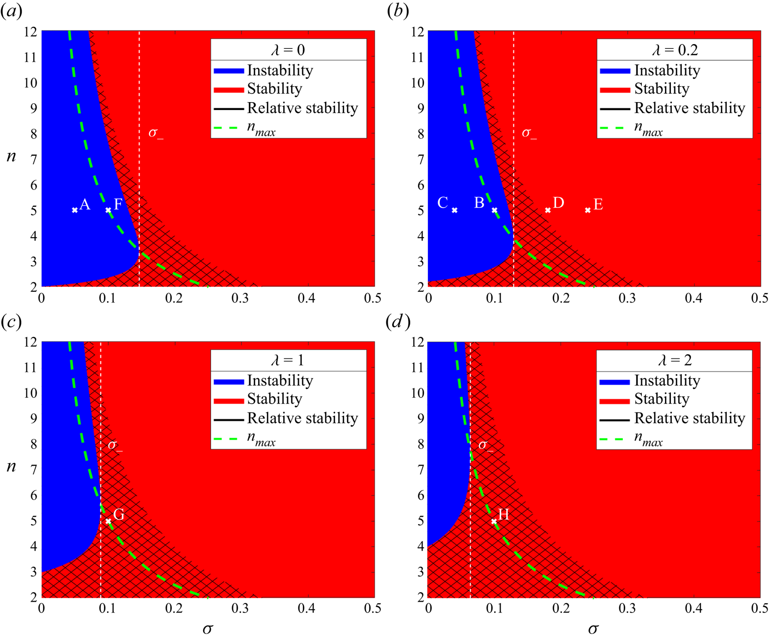
Figure 2. Parameter space stability diagrams for the perturbed fire line (3.4). Regions of instability are in blue, regions of stability are in red, and the cross-hatched areas (denoted by the black line in the graph key) are regions of ‘relative stability’. The points A–H correspond to initial choices of  $\sigma$ and $n$ in figures in § 4 as follows: A – figure 3; B – figures 4, 5(b), 7(b); C – figure 5(a); D – figure 5(c); E – figure 5(d); F – figure 7(a); G – figure 7(c); H – figure 7(d).
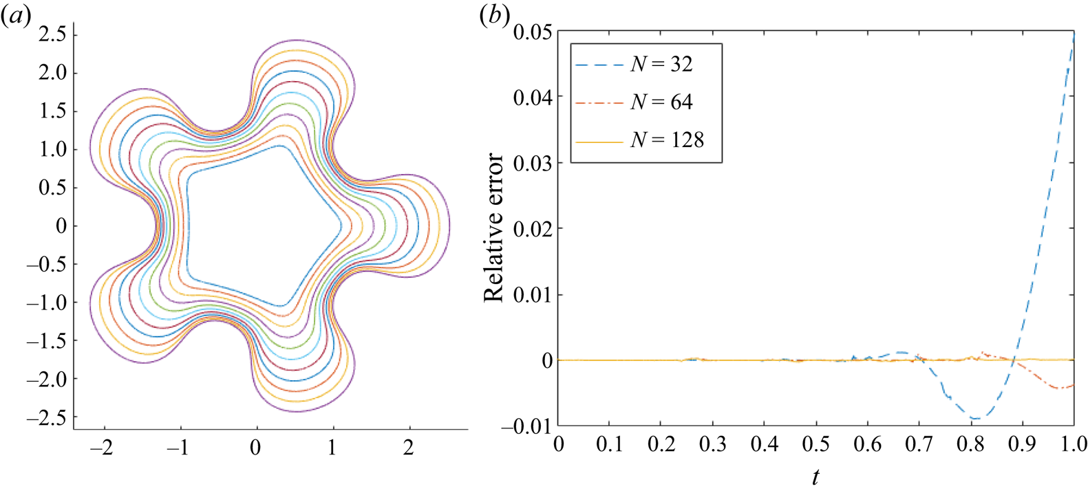
Figure 3. (a) Evolution of fire fingers for a fire-star  $n=5$ with $V_0=0$, $\bar {\epsilon }=0.1$, $\textit {Pe}_0=2$, $\lambda =0$, $\sigma _0=0.05$, $N=128$ and $t_{max}=1$. (b) Relative error of the rate of change of area law (4.8) of plot (a), for varying $N$.
$N$.

Figure 4. (a) Evolution of fire fingers for a fire-star  $n=5$ with $V_0=1$, $\bar {\epsilon }=0.5$, $\textit {Pe}_0=5$, $\lambda =0.2$, $\sigma _0=0.1$, $N=128$ and $t_{max}=2$. (b) Relative error of the rate of change of area law (4.8) of plot (a), for varying $N$.
$N$.
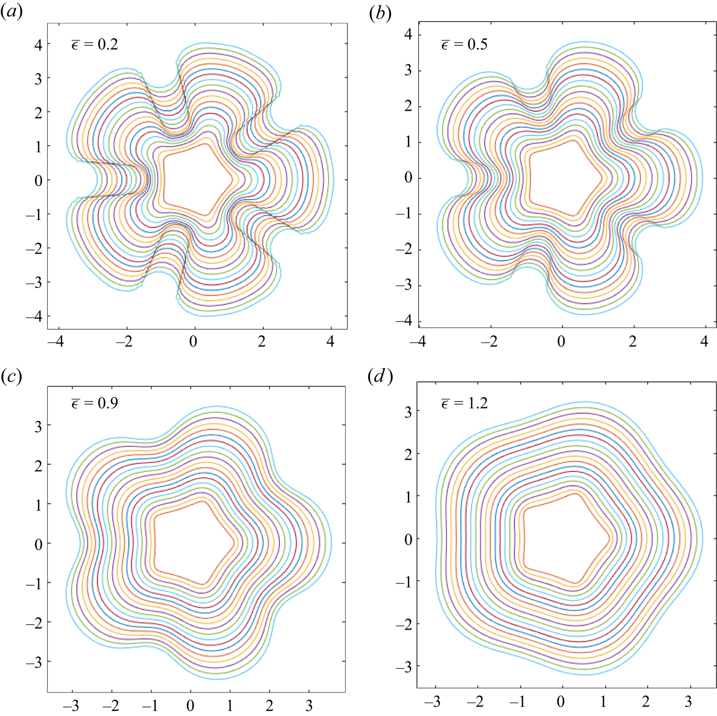
Figure 5. The effect of increasing  $\bar {\epsilon }$: evolution of a fire-star with $n=5$, $V_0=1$, $\textit {Pe}_0=5$, $\lambda =0.2$, $N=128$, $t_{max}=2$ and: (a) $\bar {\epsilon }=0.2$, $\sigma _0=0.04$; (b) $\bar {\epsilon }=0.5$, $\sigma =0.1$; (c) $\bar {\epsilon }=0.9$, $\sigma =0.18$; (d) $\bar {\epsilon }=1.2$, $\sigma =0.24$.
4. Numerical simulation of nonlinear evolution
4.1. Conformal mapping method
A numerical method based on conformal mapping is used to compute the nonlinear evolution of the fire line  $\gamma$. Let $z=f(\zeta,t)$ map the interior of the unit $\zeta$-disk to $\varOmega$, with $\zeta =0$ mapping to infinity. Conformal invariance of (2.9) and (2.10), along with boundary conditions $\phi \to \log |\zeta |$, $c=1$ as $\zeta \to 0$, and $\phi =0$, $c=0$ on $|\zeta |=1$, enables solutions for $\phi$ and $c$ to be found in the $\zeta$-plane:
 \begin{equation} \phi(\zeta) = \log{|\zeta|},\quad c(\zeta) = 1-|\zeta|^{\textit{Pe}}. \end{equation}
The numerical task is now to find the conformal map  $z=f(\zeta,t)$. As in other free-boundary problems such as Hele-Shaw flow and dissolution of solids in potential flow, the kinematic condition (2.8) is formulated in terms of the conformal map $z=f(\zeta,t)$, yielding an equation of the Polubarinova–Galin class (e.g. Howison Reference Howison1986; Ladd et al. Reference Ladd, Yu and Szymczak2020).
Write the unknown map as
 \begin{equation} z=f(\zeta,t)=a_{{-}1}(t)\,\zeta^{{-}1}+\sum_{m=1}^{\infty} a_m(t)\,\zeta^{nm-1}, \end{equation}
where  $\varOmega$ is assumed to have $n$-fold symmetry, so the $a_m$ are real, for all $m=-1,1,2,\ldots$, when $n\geqslant 1$. Note that $a_{-1}$ is the conformal radius and is a measure of the horizontal length scale of the wild fire, thus is identical to $R(t)$ for a circular fire. Hence the Péclet number can be written as $\textit {Pe}=\textit {Pe}_0\,R(t)=\textit {Pe}_0\,a_{-1}(t)$, where $a_{-1}(0)=1$ is chosen in all numerical tests. The terms in (2.8) can be expressed in terms of the map (4.2). From Dallaston & McCue (Reference Dallaston and McCue2013),
 \begin{equation} v_n=\frac{{\rm Re}\left[f_t\overline{\zeta f_\zeta}\right]}{|f_\zeta|},\quad \kappa=\frac{{\rm Re}\left[\zeta(\zeta f_\zeta)_\zeta \overline{\zeta f_\zeta}\right]}{|f_\zeta|^{3}}, \end{equation}
and the oxygen concentration gradient is
 \begin{equation} \boldsymbol{n}\boldsymbol{\cdot}\boldsymbol{\nabla}c = {\rm Re}[n\,\bar{\boldsymbol{\nabla}}c]=2\,{\rm Re}\left[n\,\frac{\partial c}{\partial z}\right]=2\,{\rm Re}\left[\frac{\zeta f_{\zeta}}{|f_\zeta|}\,\frac{\partial c}{\partial \zeta}\,\frac{1}{f_\zeta}\right]={-}\frac{\textit{Pe}}{|f_\zeta|}\quad \text{on}\ |\zeta|=1, \end{equation}
where  $\bar {\boldsymbol {\nabla }}=2\partial _z=\partial _x -i\partial _y$, $n=n_x+in_y$ is the complex representation of the normal vector in the $z$-plane, and $f_\zeta = \partial f/\partial \zeta$. Also used is the result $n=\zeta f_\zeta /|f_\zeta |$, and that $c$ in the $\zeta$-disk is given by (4.1a,b), so $\partial c/\partial \zeta =-\textit {Pe}/2\zeta$ on $|\zeta |=1$.
Now, (4.3a,b) and (4.4) can be substituted into (2.8), and multiplying through by  $|f_\zeta |/\textit {Pe}_0$ gives
 \begin{equation} {\rm Re}\left[f_t\overline{\zeta f_\zeta}\right]={-}\frac{V_0}{\textit{Pe}_0}\,|f_\zeta|+\frac{\bar{\epsilon}}{\textit{Pe}_0}\,\frac{{\rm Re}\left[\zeta(\zeta f_\zeta)_\zeta\overline{\zeta f_\zeta}\right]}{|f_\zeta|^{2}} -a_{{-}1}(t). \end{equation}
Note that choosing  $V_0=\bar {\epsilon }=0$ is analogous to the problem of viscous fingering of a fluid with zero surface tension in a Hele-Shaw cell (e.g. Howison Reference Howison1986; Mineev-Weinstein Reference Mineev-Weinstein1998; Gustafsson & Vasil'ev Reference Gustafsson and Vasil'ev2006). Omitting the $a_{-1}(t)$ term in (4.5), i.e. when there is no oxygen effect, gives the wildfire model used in e.g. Markstein (Reference Markstein1951) and Sharples et al. (Reference Sharples, Towers, Wheeler, Wheeler and McCoy2013), and is a variant of the curve-shortening problem considered by Dallaston & McCue (Reference Dallaston and McCue2016), except that, in this case, the sign of $V_0$ is such that the curve lengthens.
Following Dallaston & McCue (Reference Dallaston and McCue2013), the series in (4.2) is truncated at  $m=N$, giving $N+1$ unknown functions in time: $a_{-1}, a_{1},\ldots,a_{N}$. Consequently, points $\zeta =\zeta _j$, $j=1,\ldots, N+1$, distributed uniformly around the $\zeta$-disk, are chosen, so (4.2) becomes a system of $N+1$ coupled first-order ODEs in $t$. Here, the MATLAB routine ode15i is used to solve this system.
4.2. Rate of change of area law
It is useful to find any identities satisfied by (2.8)–(2.12), as these can be used to assess the accuracy of the above numerical method. Let  $A(t)$ be the area enclosed by the fire line $\gamma$, and denote the length of $\gamma$ by $L(t)$. The following geometrical properties of a smooth, non-intersecting, two-dimensional closed curve $\gamma$ (Brower et al. Reference Brower, Kessler, Koplik and Levine1984; Dallaston & McCue Reference Dallaston and McCue2016) are used:
 \begin{equation} 2{\rm \pi} = \int_\gamma \kappa \,\mathrm{d} s,\quad L(t)=\int_\gamma\, \mathrm{d} s,\quad \frac{\mathrm{d} A}{\mathrm{d} t} = \int_\gamma v_n \,\mathrm{d} s. \end{equation}
Substituting (2.8) into (4.6c) gives
 \begin{equation} \frac{\mathrm{d} A}{\mathrm{d} t} = \frac{V_0}{\textit{Pe}_0}\int_\gamma \,\mathrm{d}s -\frac{\bar{\epsilon}}{\textit{Pe}_0}\int_\gamma \kappa \,\mathrm{d} s + \frac{1}{\textit{Pe}_0}\int_\gamma \frac{\partial c}{\partial n} \,\mathrm{d} s. \end{equation}
 The first two terms on the right-hand side of (4.7) can be simplified using (4.6a,b). For the third term, first transform the integral to the unit  $\zeta$-disk $\zeta ={\rm e}^{{\rm i}\theta }$, where $0\leqslant \theta <2{\rm \pi}$. Now use $\partial c/ \partial n = \textit {Pe}_0\,a_{-1}(t)/|f_{\zeta }|$, which is similar to (4.4) but necessarily positive as the normal is directed outwards to $\gamma$. Since $\mathrm {d} s = |f_{\zeta }|\,\mathrm {d}\theta$, the rate of change of area law for the burned region is obtained:
 \begin{equation} \frac{\mathrm{d} A}{\mathrm{d} t} = \frac{V_0}{\textit{Pe}_0}\,L(t)+2{\rm \pi}\left[a_{{-}1}(t)-\frac{\bar{\epsilon}}{\textit{Pe}_0}\right]. \end{equation}
The relation (4.8) is used to check the accuracy of the numerical results using the relative error
 \begin{equation} RE = \frac{{\rm LHS}-{\rm RHS}}{{\rm RHS}}, \end{equation}
where LHS and RHS are the left- and right-hand sides of (4.8), respectively.
4.3. Results
4.3.1. Fire-stars
The nonlinear evolution of a 5-fold symmetric shape ( $n=5$), or fire-star, is computed. First, consider the case with zero ROS, $V_0=0$, and small curvature effect, $\bar {\epsilon }=0.1$. The initial Péclet number $\textit {Pe}_0=2$ is chosen, thus $\lambda =V_0/\textit {Pe}_0=0$ and $\sigma _0=\bar {\epsilon }/\textit {Pe}_0=0.05$, corresponding to point A on the stability diagram figure 2(a). The series (4.2) is truncated at $N=128$ terms, and the fire line evolves to $t_{max}=1$; this evolution is shown in figure 3(a). Sections of the fire line penetrating the unburned region grow more quickly, and fingers develop from the tips of the initial perturbations. This behaviour is in agreement with the stability diagram, in which this evolution begins in the instability region and remains unstable as $\sigma$ decreases over time, as a result of an increasing Péclet number. In addition, instability is also expected owing to the Mullins–Sekerka mechanism (Mullins & Sekerka Reference Mullins and Sekerka1964; Brower et al. Reference Brower, Kessler, Koplik and Levine1984).
The relative error  $RE$ (see (4.9)) of the rate of change of area law (4.8) for figure 3(a) is plotted in figure 3(b). Each of the three plots corresponds to a different value of series truncation: $N=32$, $64$ and $128$, where the higher the series truncation, the further in time the fire line can evolve before significant numerical errors appear. The cause of these errors is likely the lack of resolution in the ‘valleys’ of the fingers, due to a crowding of points at the ‘finger tips’. While the points in the $\zeta$-plane are distributed uniformly, when mapped with (4.2) to the $z$-plane, their distribution becomes non-uniform around the fire line, hence the crowding. Evolution with larger $\bar {\epsilon }$ and $V_0$ can be computed accurately for larger times; the stronger curvature effect means that finger formation, and consequent crowding, take longer to develop.
Figure 4(a) gives an example of a more stable case; its initial state is the same as that of figure 3(a), but now with  $V_0=1$, $\bar {\epsilon }=0.5$, $\lambda =0.2$ and $\sigma _0=0.1$, and evolving up to a time $t_{max}=2$. The burned area $R$ grows to a larger size due to the non-zero $V_0$, and though fingers still develop as predicted in the stability diagram figure 2(b) (point B), they are less pronounced compared with figure 3(a), due to the $V_0$ and increased $\bar {\epsilon }$ effects. Also, the relative errors plotted in figure 4(b) are significantly smaller in magnitude than those in figure 3(b), with $RE$ decreasing as $N$ is increased. Henceforth, all plots will use $N=128$, unless stated otherwise.
The result of increasing the curvature effect is shown in figure 5 for four choices of  $\bar {\epsilon }$. As expected (Sethian Reference Sethian1985; Hilton et al. Reference Hilton, Miller, Sharples and Sullivan2016), increasing $\bar {\epsilon }$ smooths the fire line, reducing the amplitude of the fingers and valleys. The value $\lambda =0.2$ is chosen, hence the stability diagram figure 2(b) is considered, with figures 5(a–d) corresponding to the points C, B, D and E, respectively. Figures 5(a,b) are unstable, and figure 5(d) is stable, in agreement with the initial position of each experiment in figure 2(b).
However, in figure 5(c), while perturbations seem to decay at first, eventually the fingers grow to an amplitude larger than the initial perturbations. Considering figure 2(b), the fire starts at point D in the stability region, but as  $\sigma$ decreases, the fire enters the instability regime. This is known as a ‘dormant fire instability’, as the fire fingers appear to recede before growing again. Eventually, any initially stable fire line will become unstable as $\textit {Pe}$ will continue to grow; the physical likelihood of this is discussed in § 6. Figure 6(a) gives an example of a dormant fire instability of a 7-pointed ( $n=7$) fire-star. The corresponding translation of the fire line on the stability diagram is also shown in figure 6(b) as a white line with markers at each time step of $1.25$. The value of $\lambda$ is zero, and initially, $\sigma =0.25$, so the fire line is stable at $t=0$ and perturbations decay. At $t=1.25$, perturbations start to grow, but are slower than the overall growth of the wildfire; the fire line does not become unstable until around $t=1.8$, when $\sigma =0.106$. However, fire fingers do not become apparent until $t=5$.

Figure 6. (a) The evolution of a dormant fire instability of a 7-pointed star with  $n=7$, $V_0=0$, $\bar {\epsilon }=0.5$, $\textit {Pe}_0=2$, $\lambda =0$, $\sigma _0=0.25$, $N=128$ and $t_{max}=10$. (b) The parameter space stability diagram of (a); each marker represents a time step of $t=1.25$, from $t=0$ (furthest right) to $t=6.25$ (furthest left).
Finally, the effect of increasing  $V_0$ on fire line evolution is shown in figure 7, where figures 7(a–d) correspond to the points F, B, G and H in figures 2(a–d), respectively. Increasing $V_0$ in the stability diagrams of figure 2 ‘thins’ and shifts the instability region such that instability is not achieved until smaller values of $\sigma$ are reached, and some lower modes, such as $n=3$, may always be relatively stable. In the case of fire-stars ( $n=5$) with $\lambda \leqslant 2$, however, instability is always eventually realised. Note that although figure 7(d) looks almost circular, distinct valleys are still observed; increasing $V_0$ causes fire fingers to widen, but not necessarily to flatten.

Figure 7. The effect of increasing  $V_0$: evolution of a fire-star with $\bar {\epsilon }=0.5$, $\textit {Pe}_0=5$, $N=128$, $t_{max}=2$ and: (a) $V_0=0$, $\lambda =0$; (b) $V_0=1$, $\lambda =0.2$; (c) $V_0=5$, $\lambda =1$,; (d) $V_0=10$, $\lambda =2$.
4.3.2. Fire lines with elliptical starting shapes
In addition to slightly perturbed circular fire lines (as in § 3), for example the fire-stars previously considered, the numerical method is also able to compute the evolution of fire lines with non-small initial perturbations. For the sake of illustration, here elliptical starting shapes are considered, that is,  $\gamma$ is a $2$-fold ( $n=2$) symmetric curve that corresponds to an ellipse with eccentricity $e$. As $e\rightarrow 1$, the minor axis of the ellipse approaches $0$, so the ellipse tends towards a slit. Choosing an eccentricity close to $1$ provides an approximation of the evolution of a one-dimensional fire line segment. As perturbations are non-small, the stability analysis of § 3 is not relevant in this case.
Figure 8 shows a series of results for initial ellipses with  $e=0.9986$, all of which use $N=128$, $t_{max}=9$ and $\textit {Pe}_0=2$. The effect of increasing $V_0$ is shown in figures 8(a–c). As in figure 7 for a fire-star, the fires grow to a larger conformal radius as $V_0$ increases, as noted by the axis scales in each figure. There is also evidence of finger widening; however, as there are only two fingers, this is seen as the valley between the fingers decreasing in depth and width, but still the valley is preserved. Flattening of the fingers is achieved by increasing the curvature effect, as seen in figure 8(d), where $\bar {\epsilon }$ has increased to $0.9$, as opposed to $0.5$ for the other plots in figure 8. Finally, numerical instabilities are visible in figure 8(a) at around $t=7$, due to the high curvature of the developing valleys. The model fails when the fire line begins to intersect previous iterations of itself from $t=8$ onwards. This violates the entropy condition (Sethian Reference Sethian1985), hence the results are unphysical from this time; results are displayed up to $t_{max}=9$ to show the self-intersection of the fire line more clearly.

Figure 8. Evolution of an initially elliptical fire line with  $\textit {Pe}_0=2$, $N=128$, $t_{max}=9$, $e=0.9986$ and: (a) $V_0=0$, $\bar {\epsilon }=0.5$, $\sigma _0=0.25$; (b) $V_0=1$, $\bar {\epsilon }=0.5$, $\sigma _0=0.25$; (c) $V_0=5$, $\bar {\epsilon }=0.5$, $\sigma _0=0.25$; (d) $V_0=1$, $\bar {\epsilon }=0.9$, $\sigma _0=0.45$.
4.3.3. Emergence of a dominant mode
So far, only one mode of perturbation has been induced on a circular fire line; for fire-stars, this was the mode  $n=5$ (or $n=7$ for a $7$-pointed star), and for an ellipse it was $n=2$. Now, multiple modes of (small) perturbation will be imposed at once, and the resulting evolution explored. To allow many (co-prime) modes to be added, only $1$-fold symmetry ( $n=1$) is assumed; this means that the coefficients of (4.2) are still real and hence solvable in the current numerical method. It is expected that one mode will eventually dominate, for example the mode $n=n_{max}$ (see § 3) that has the highest growth rate $g_{max}$ of all possible modes for a given $\sigma$. In general, the mode with the highest growth rate of all excited modes will dominate. Since the Péclet number is increasing, and so $\sigma$ is decreasing, this dominant mode changes over time, as noted in § 3.
First consider the case where  $\textit {Pe}$ is a constant in time; this differs from the radial fire model but means that the values of $\sigma$, and hence $n_{max}$, are unchanging. Much of the working remains the same as in § 3, with $\sigma =\bar {\epsilon }/\textit {Pe}={\rm const}.$, and the only difference to the governing equation (4.5) is a $-1$ term rather than $-a_{-1}(t)$. Perturbations incorporating $n=3$, $5$ and $7$ modes are induced, each of small and equal amplitude, to an initially circular fire line. Fire line evolution is computed up to $t_{max}=9$ with zero ROS ( $V_0=0$) and a series truncation $N=128$. Figures 9(a–c) show the results for the different choices of $\sigma =0.08$, $0.1$ and $0.14$, respectively. In each plot, a different dominant mode emerges: when $\sigma =0.08$ (figure 9a), the $7{\text {th}}$ mode dominates; for $\sigma =0.1$ (figure 9b), it is the $5{\text {th}}$ mode; and (c) for $\sigma =0.14$ (figure 9c), it is the $3{\text {rd}}$ mode. This agrees with the stability diagram in figure 9(d); for each choice of $\sigma$, the positions of the $3{\text {rd}}$-, $5{\text {th}}$- and $7{\text {th}}$-order perturbations are plotted as nodes. For $\sigma =0.1$, $n=5$ is exactly $n_{max}$. For $\sigma =0.08$, $n=7$ has the highest growth rate of the three perturbations and hence dominates; and similarly for $n=3$ in the $\sigma =0.14$ case.

Figure 9. (a–c) Evolution of a fire line with  $3{\text {rd}}$-, $5{\text {th}}$- and $7{\text {th}}$-order perturbations and $\textit {Pe}$ constant. Here, $V_0=0$, $\textit {Pe}_0=5$, $\lambda =0$, $t_{max}=9$, $N=128$, and (a) $\sigma =0.08$, (b) $\sigma =0.1$, (c) $\sigma =0.14$. (d) Stability diagram; each vertical, dashed line represents the $\sigma$ value for results in (a–c) (from left to right), and each node on these vertical lines represents the $3{\text {rd}}$-, $5{\text {th}}$- and $7{\text {th}}$-order perturbation terms.
Now consider when  $\textit {Pe}=\textit {Pe}_0\,a_{-1}(t)$. As $\sigma$ decreases, the value of $n_{max}$ (see (3.16a)) increases, so it is expected that the highest numbered excited mode will dominate eventually – though it should be cautioned that once perturbations grow sufficiently large, they are no longer ‘small’ and so the stability analysis of § 3 can no longer be expected to hold. Numerical experiments in figure 10 show the evolution of the same initial fire line as in figure 9, with the same initial conditions $V_0=0$ and $N=128$, but with different choices of $\sigma _0$. The value of $t_{max}$ in each experiment corresponds to the maximum time possible before the simulation fails.

Figure 10. Evolution of the initial fire line in figure 9 for a time-dependent  $\textit {Pe}$, with $V_0=0$ and $N=128$: (a) $\sigma _0=0.14$, $\sigma _f=0.04$, $t_{max}=2.5$; (b) $\sigma _0=0.02$, $\sigma _f=0.033$, $t_{max}=5.2$.
There is immediately a difference compared to the constant  $\textit {Pe}$ case. Figure 10(a) has the same starting value $\sigma _0=0.14$ as in figure 9(c), yet now the $7{\text {th}}$-order perturbation dominates, not the $3{\text {rd}}$, with the final value of $\sigma$ as $\sigma _f=0.04$. The fire fingers grow faster too, achieving a similar result to figure 9(a) but at a quicker time $t=2.5$. Any lower initial values of $\sigma _0$ also result in the $7{\text {th}}$-order perturbation dominating. In figure 10(b), $\sigma _0=0.2$, and it is the $5{\text {th}}$-order perturbation that dominates, with the simulation terminating at $t_{max}=5.2$ when $\sigma _f=0.033$. The fact that this mode dominates over the higher $n=7$ mode seems to contradict what is expected, though it is likely that the numerical method ended before the $n=7$ mode could begin to grow sufficiently. Close inspection of figure 10(b) suggests that there are in fact seven fingers growing, not five.
5. Periodic infinite fire lines
Infinite fire lines are now considered, and this can be thought of as studying a sufficiently large wildfire at a local scale. In particular, a periodic curve  $\gamma _L$ is considered over one period $[-L{\rm \pi},L{\rm \pi} ]$, with $L$ a characteristic length scale used to convert to non-dimensional quantities. The dimensionless system (2.8)–(2.12) used for radial fire lines also holds in the periodic infinite case, but with two main changes. First, as a local scale is considered, it is assumed that the strength $Q$ of the fire plume remains constant over time as the fire line propagates forward. Therefore, the Péclet number is also constant, hence $\textit {Pe}=\textit {Pe}_0$ always. Second, the far-field condition (2.12b) is now that of a uniform flow in the negative $\hat {\boldsymbol {y}}$ direction, as the effective oxygen sink is now on the line $y=R(t)$, which draws in oxygen-rich air from the unburned region at $y\to +\infty$. Note that $R(t)$ is not a radius; rather, it is the horizontal line $y=R(t)$.
The non-dimensional system for periodic infinite fire lines is thus
 \begin{gather} \textit{Pe}\,v_n=V_0 -\bar{\epsilon}\kappa+\hat{\boldsymbol{n}}\boldsymbol{\cdot}\boldsymbol{\nabla}c\quad \text{on }\gamma_L, \end{gather}
 \begin{gather}\nabla^{2}\phi=0\quad \text{in }\varOmega, \end{gather}
 \begin{gather}\textit{Pe}\,\boldsymbol{u}\boldsymbol{\cdot}\boldsymbol{\nabla} c=\nabla^{2} c \quad \text{in }\varOmega, \end{gather}
 \begin{gather}c=0,\quad \phi=0\quad \text{on }\gamma_L, \end{gather}
 \begin{gather}c\rightarrow 1,\quad v\rightarrow-1\quad \text{as }y\rightarrow\infty. \end{gather}
The problem is shown diagrammatically in figure 11.

Figure 11. The dimensionless wildfire problem for a periodic infinite fire line.
5.1. Stability analysis
As in § 3, consider first an unperturbed base case  $y=R(t)$. Assuming that $\phi$ and $c$ are independent of $x$, the following solve (5.1)–(5.5a,b):
 \begin{equation} \phi(y)=R(t)-y,\quad c(y)=1-\exp({\textit{Pe}\,(R(t)-y)}). \end{equation}
 Next, perturbations  $y=y_p=R(t)+\delta _n\cos {nx}$ are added, where the summation sign has been dropped and $\delta _n\ll 1$, for all $n=1,2,3,\ldots$. Note that $n=1$ is not a simple translation as in the radial case, hence perturbations $n\geqslant 1$ are retained here. The following solutions for $\phi$ and $c$ are assumed:
 \begin{equation} \left.\begin{gathered} \phi(x,y) = R(t)-y+\beta_n \exp({n(R(t)-y)})\cos{nx},\\ c(x,y)=1-\exp({\textit{Pe}\,(R(t)-y)})+\gamma_n \exp({\alpha_n(R(t)-y)})\cos{nx}, \end{gathered}\right\} \end{equation}
with constants  $\beta _n,\gamma _n\ll 1$ and $\alpha _n$. Substitution of (5.7) into (5.3) and (5.4a,b) gives $\beta _n=\delta _n$, $\gamma _n=-\textit {Pe}\,\delta _n$ and $\alpha _n=n+\textit {Pe}$.
The normal velocity (2.8) can be written in terms of  $y_p$ as
 \begin{equation} \textit{Pe}\,(\dot{R}+\dot{\delta_n}\cos{nx})=V_0-\bar{\epsilon}n^{2}\delta_n\cos{nx}+\textit{Pe}\,[1+n\delta_n\cos{nx}]. \end{equation}
Extracting the first-order terms gives
 \begin{equation} \textit{Pe}\,\dot{R}=V_0 +\textit{Pe}, \end{equation}
and an exact solution for  $R$ can be found:
 \begin{equation} R(t)=(\lambda+1)t, \end{equation}
where  $\lambda =V_0/\textit {Pe}$ and the condition $R(0)=0$ has been imposed. The relative growth of the fire line is therefore
 \begin{equation} \frac{\dot{R}}{R}=\frac{1}{R}\,(\lambda+1)=\frac{1}{t}, \end{equation}
which eliminates the parameter  $\lambda$, and thus $V_0$, from the stability analysis. Next, the ${O}(\delta _n)$ terms from (5.8) are taken, giving
 \begin{equation} \textit{Pe}\,\dot{\delta_n}={-}\bar{\epsilon}n^{2}\delta_n+n\,\textit{Pe}\,\delta_n, \end{equation}
thus
 \begin{equation} \frac{\dot{\delta_n}}{\delta_n}=n(1-\sigma n), \end{equation}
where  $\sigma =\bar {\epsilon }/\textit {Pe}$ is a constant in time.
Therefore the relative growth rate is
 \begin{equation} g(n)=\frac{\partial}{\partial t}\left(\log{\left(\frac{\delta_n}{R}\right)}\right)=\frac{\dot{\delta_n}}{\delta_n}-\frac{\dot{R}}{R} = n(1-\sigma n)-\frac{1}{t}. \end{equation}
As in § 3,  $g(n)>0$ is unstable behaviour, $g(n)\leqslant 0$ implies stability, and ‘relative stability’ is when ${\dot \delta _n}/\delta _n>0$ but $g(n)\leqslant 0$. Care must also be taken at $t=0$, though it is only the sign of (5.14) that is important, so state simply that $g<0$ at $t=0$, for all $n$. Whereas the growth rate of radial fires (3.11) was variable in $n$ and $\sigma$, with $\sigma$ decreasing over time, now $\sigma$ is a constant and the growth rate for periodic infinite fire lines (5.14) is explicitly time-dependent, approaching the standard growth rate (5.13) as $t$ increases. Therefore, the resulting stability diagrams, as given in figure 12, have axes $n$ versus $t$, rather than $n$ versus $\sigma$, with a constant value of $\sigma$ chosen for each plot. The maximum growth rate $g_{max}$ and its corresponding mode $n_{max}$ are also found as
 \begin{equation} n_{max}=\frac{1}{2\sigma},\quad g_{max} = \frac{1}{4\sigma}-\frac{1}{t}. \end{equation}
The lines A–D identified in figure 12 correspond to upcoming numerical results that all run from  $t=0$ to $t=5$, i.e. tracing from left to right on the stability diagram.

Figure 12. Parameter space stability diagrams for the perturbed periodic infinite fire line. The cross-hatched areas (denoted by the black line in the graph key) are regions of ‘relative stability’. The lines A–D represent upcoming numerical results, which run from  $t=0$ to $t=5$, as follows: A – figure 13(a); B – figures 13(b) and 14; C – figure 13(c); D – figure 13(d).

Figure 13. The effect of increasing  $\bar {\epsilon }$: evolution of a periodic infinite fire line with $V_0=1$, $\textit {Pe}=2$, $N=128$, $t_{max}=5$ and: (a) $\bar {\epsilon }=0.2$, $\sigma =0.1$; (b) $\bar {\epsilon }=0.5$, $\sigma =0.25$; (c) $\bar {\epsilon }=1.5$, $\sigma =0.75$; (d) $\bar {\epsilon }=2.5$, $\sigma =1.25$.

Figure 14. The effect of increasing  $V_0$: evolution of a periodic infinite fire line with $\bar {\epsilon }=0.5$, $\textit {Pe}=2$, $\sigma =0.25$, $N=128$, $t_{max}=5$, and (a) $V_0=0$, (b) $V_0=1$, (c) $V_0=2$, (d) $V_0=5$.
Figure 14 shows the effect of increasing the ROS, comparing the values  $V_0=0, 1, 2,5$, with $\textit {Pe}=2$, $\bar {\epsilon }=0.5$, $\sigma =0.25$, $N=128$ and $t_{max}=5$ for all plots. All figures correspond to and agree with the line B in the stability diagram figure 12(b), showing that each result is unstable after the first few time steps. Increasing $V_0$ causes the fire line to propagate faster and the finger to widen; the finger in figure 14(d) covers almost the entire period.
5.2. Numerical results
The conformal mapping method from § 4.1 is used again to produce numerical results. For one period of a periodic infinite fire line, the following conformal map from the interior of the unit  $\zeta$-disk to the unburned region $\varOmega$ is used:
 \begin{equation} z=f(\zeta,t)={-}{\rm i}\log{\zeta}+{\rm i}\,a_0(t)+{\rm i}\sum_{m=1}^{\infty} a_m(t)\,\zeta^{m}. \end{equation}
Symmetry about the  $y$-axis is assumed, so the unknowns $a_m$ are real.
The normal velocity  $v_n$ (see (5.1)) is evaluated as in § 4 to give
 \begin{equation} {\rm Re}\left[f_t\overline{\zeta f_\zeta}\right]={-} \frac{V_0}{\textit{Pe}}\,|f_\zeta|+\frac{\bar{\epsilon}}{\textit{Pe}}\,\frac{{\rm Re}\left[\zeta(\zeta f_\zeta)_\zeta\overline{\zeta f_\zeta}\right]}{|f_\zeta|^{2}} -1, \end{equation}
with the  $-1$ term rather than the $a_{-1}(t)$ in (4.5), as $\textit {Pe}$ is now not scaled in time. For all upcoming results, the initial fire line is a straight-line segment with a simple ‘bump’, i.e. a perturbation of $n=1$. Also, the axes have been inverted ( $y$ is the horizontal) to show the evolution more clearly.
Figure 13 shows the effect of increasing the curvature by comparing the values  $\bar {\epsilon }=0.2$, 0.5, 1.5 and $2.5$, with $\textit {Pe}=2$, $V_0=1$, $N=128$ and $t_{max}=5$ for all plots. Similar to radial fire line evolution, such as in figures 13(a,b), as the curvature effect increases, the finger grows more slowly until eventually the curvature is strong enough to stop finger growth altogether as in figure 13(d). Note also that for small curvature, e.g. in figure 13(a) ( $\bar {\epsilon }=0.2$), numerical instabilities appear eventually. This is again likely due to crowding. Considering stability, figures 13(a–d) correspond to the lines A, B, C and D across the stability diagrams figures 12(a–d), respectively. The only stable solution is in figure 13(d), where $\bar {\epsilon }=2.5$; this is in agreement with figure 12, as line D is the only experiment never to enter the instability region for $0\leqslant t\leqslant 5$.
6. Discussion
The stability and nonlinear evolution of radial and infinite fire lines have been considered using a two-dimensional model incorporating both geometric and dynamic effects. Fingering instabilities are possible for certain values of  $\sigma$, the ratio between curvature $\bar {\epsilon }$ (stabilising) and oxygen $\textit {Pe}$ (destabilising) effects, and numerical results demonstrate both stable and unstable fire line growth. A third type of behaviour was also found: ‘dormant fire’ behaviour, where fire finger growth would change from stable to unstable over time. This was a consequence of an increasing Péclet number in the radial case. In cases where multiple modes of perturbation were excited, the mode with the highest growth rate would dominate eventually. Consequently, geometrically identical initial fire lines evolve into different fire finger patterns, depending on the value of $\sigma$.
Using  $L\approx 20$ m for the initial size of a radial fire that generates a fire wind of $0.025\ \textrm {m~s}^{-1}$ gives an initial estimate $Q=2{\rm \pi} \times 0.5\ \textrm {m}^{2}\ \textrm {s}^{-1}$. These values are consistent with large-scale experimental grass fires reported in Hilton et al. (Reference Hilton, Sullivan, Swedosh, Sharples and Thomas2018). Bebieva et al. (Reference Bebieva, Oliveto, Quaife, Skowronski, Heilman and Speer2020) estimate that within 1 m of ground level, the horizontal diffusivity $D$ in fire conditions is ${{O}}(1)\ \textrm {m}^{2}\ \textrm {s}^{-1}$, although the actual value will depend on vegetation type, among other factors. Hence $\textit {Pe}_0=Q/2{\rm \pi} D\approx 0.5$. The value of $\bar {\epsilon }$ is more difficult to estimate. In the combustion wind tunnel experiments discussed by Hilton et al. (Reference Hilton, Miller, Sharples and Sullivan2016) (see e.g. their figure 6), fires typically have length scale 0.5 m, and they found by comparison with their numerical experiments (which included curvature) that dimensionally, the curvature term's contribution to the normal velocity is $\approx 2\times 10^{-4}\ \textrm{m s}^{-1}$. In the same experiments, a typical fire line velocity in the absence of wind was $3\times 10^{-3}\ \textrm {m~s}^{-1}$, so ${{\bar \epsilon }\approx 0.1}$. Thus choosing this value as being representative of larger scale fire, it follows that $\sigma _0={\bar \epsilon }/{\textit {Pe}_0}\approx 0.2$. With caveats about applying these estimates to larger-scale fires and questions about how different fuel types and vegetation affect wildfires, the estimate for $\sigma _0$ suggests that fingering owing to the oxygen effect is a possibility in actual wildfires.
The fire line normal velocities (2.8) and (5.1) are extensions of the curvature flow models used by e.g. Sharples et al. (Reference Sharples, Towers, Wheeler, Wheeler and McCoy2013) and Sethian (Reference Sethian1985), with the added term  $\boldsymbol {\hat {n}}\boldsymbol {\cdot }\boldsymbol {\nabla }c$ modelling the effect of additional oxygen supplied to the fire by advection and diffusion. While the diffusion and advection of oxygen concentration in relation to fires has been acknowledged (Zik et al. Reference Zik, Olami and Moses1998; Conti & Marconi Reference Conti and Marconi2002), and the phenomenon of fire wind is well known (Smith et al. Reference Smith, Morton and Leslie1975; Beer Reference Beer1991; Hilton et al. Reference Hilton, Sullivan, Swedosh, Sharples and Thomas2018), the explicit inclusion of the oxygen term in the normal velocity of the fire line is new. Mathematically, the model combines aspects of curve-shortening flow (Dallaston & McCue Reference Dallaston and McCue2016), fingering in a Hele-Shaw cell in the absence of surface tension (Howison Reference Howison1986; Mineev-Weinstein Reference Mineev-Weinstein1998; Gustafsson & Vasil'ev Reference Gustafsson and Vasil'ev2006), and two-dimensional melting/freezing free-boundary problems featuring the advection–diffusion equation (2.10) (e.g. Cummings et al. Reference Cummings, Hohlov, Howison and Kornev1999; Rycroft & Bazant Reference Rycroft and Bazant2016; Ladd et al. Reference Ladd, Yu and Szymczak2020).
Several extensions to the model are of interest. Wildfires are affected strongly by ambient winds, and their inclusion would give rise to two effects. The first is a contribution to the ROS, taking the form  ${\boldsymbol {V}} \boldsymbol {\cdot }\hat {{\boldsymbol {n}}}$, where $V$ is the ambient wind, while taking care to ensure that the fire line does not turn back on itself towards the burned region (e.g. Hilton et al. Reference Hilton, Sullivan, Swedosh, Sharples and Thomas2018). The second effect is the ability of an ambient wind to transport additional oxygen to the fire line. Interestingly, Beer (Reference Beer1991) argues that in the presence of an ambient wind, the fire wind generated by the rising hot air over the burned region is reduced, and in turn, so is the instability mechanism of enhanced oxygen at the fire front. Depending on their direction, ambient winds may also transport oxygen from the burned regions to the fire line. This provides a stabilising effect since now the finger tips receive comparatively less oxygen than the valleys between fingers.
Other effects that are possible to incorporate into the model include the variance of ROS depending on whether the fire is propagating upslope or downslope, and the effect of inhomogeneous fuel and firebreaks. All these effects can be modelled by spatially dependent normal velocities, and are relatively straightforward to include in the numerical technique. To enable accurate computation of fire line evolution over longer times, an approach based on approximating the fire line as a many-sided polygon in which nodes can be added (or subtracted) according to local curvature, and in which fire lines can merge, is being developed presently. Consideration of the fire line as a polygon means that it can be mapped numerically to a canonical domain in order to facilitate the calculation of the oxygen diffusion and advection effect.
In real wildfires, fire fingers are only occasionally observed, despite the prediction here that all radial fires must eventually become unstable as  $\textit {Pe}$ increases with fire size. In reality, it seems likely that the strength of the fire wind cannot grow indefinitely and that there is a bound on $\textit {Pe}$, meaning that a fire may remain stable. Moreover, inclusion of additional factors affecting fire spread, such as ambient winds, topography, natural and artificial fire breaks, fuel type and fire spotting, may inhibit or mask finger formation.
Acknowledgements
The authors are grateful to the referees for their helpful suggestions.
Funding
S.J.H. was supported by a UK Engineering and Physical Sciences Research Council PhD studentship, grant nos EP/N509577/1 and EP/T517793/1.
Declaration of interests
The authors report no conflict of interest.


 Open access